Feature selection for hybrid information systems based on fuzzy β covering and fuzzy evidence theory

Abstract

Feature selection can remove data noise and redundancy and reduce computational complexity, which is vital for machine learning. Because the difference between nominal attribute values is difficult to measure, feature selection for hybrid information systems faces challenges. In addition, many existing feature selection methods are susceptible to noise, such as Fisher, LASSO, random forest, mutual information, rough-set-based methods, etc. This paper proposes some techniques that consider the above problems from the perspective of fuzzy evidence theory. Firstly, a new distance incorporating decision attributes is defined, and then a relation between fuzzy evidence theory and fuzzy β covering with an anti-noise mechanism is established. Based on fuzzy belief and fuzzy plausibility, two robust feature selection algorithms for hybrid data are proposed in this framework. Experiments on 10 datasets of various types have shown that the proposed algorithms achieved the highest classification accuracy 11 times out of 20 experiments, significantly surpassing the performance of the other 6 state-of-the-art algorithms, achieved dimension reduction of 84.13% on seven UCI datasets and 99.90% on three large-scale gene datasets, and have a noise tolerance that is at least 6% higher than the other 6 state-of-the-art algorithms. Therefore, it can be concluded that the proposed algorithms have excellent anti-noise ability while maintaining good feature selection ability.

Keywords

Feature selection fuzzy β covering fuzzy belief fuzzy plausibility hybrid information systems

1 Introduction

1.1 Research background and related works

Feature selection is an essential means to enhance the performance of learning algorithms, and also a crucial data preprocessing step in pattern recognition. Feature selection methods can be divided into two categories: filtering and packaging techniques, depending on their independence from subsequent learning algorithms. Filtering techniques are independent of subsequent learning algorithms and directly utilize the statistical properties of all training data to evaluate features, such as Fisher, mutual information, rough-set-based approaches, etc. Their advantage is fast speed, but they are highly susceptible to noise. Wrapper techniques use the training accuracy of subsequent learning algorithms to evaluate subsets of features, such as random forest, recursive feature elimination, etc. Their advantage is that the error is low, but they are not suitable for large datasets due to the high amount of computation involved.

An important application of rough set theory is feature selection in data analysis. Due to the presence of numerous redundant features and noise in many datasets, feature selection is necessary prior to data mining. Feature selection is an important “data preprocessing” step. It can not only reduce the size of the dataset but also enhance the accuracy of knowledge discovery. Currently, research focus on how to develop a better heuristic function to evaluate the importance of features in a dataset [1].

Rough set theory can be used for processing imprecise, inconsistent, and incomplete information [2]. It is widely used for feature selection without any prior knowledge [3]. Due to strict equivalence requirements, traditional rough set theory is only suitable for discrete data. Most real data are continuous, such as gene expression data and sensor data. If continuous data is transformed into categories through discretization, some information loss may occur.

To solve the above problem, Lynn et al. [4] built a neighborhood rough set model by substituting a neighborhood relation for an equivalence relation. They defined a neighborhood operator by using a mapping $N : U \to P (U)$ ( $P (U)$ represents the collection of subsets of U). This operator no longer requires the equality of attribute values, so the result is no longer the equivalence class of the object [4]. Dubois et al. [5] established a fuzzy rough set model with the advantages of both fuzzy sets and rough sets. These two models are common and effective methods to deal with continuous data, and many feature selection algorithms based on them are proposed. Hu et al. [6] used neighborhood rough sets for feature selection of heterogeneous data by a heuristic function called feature dependency. Zhang et al. [7] put forward an attribute reduction algorithm using evidence theory and neighborhood rough sets. Wang et al. [8] used the local conditional information entropy for feature selection based on the neighborhood rough sets. Wang et al. [9] defined the decision self-information based on neighborhood rough sets and used it for feature selection. Sun et al. [10] proposed a feature selection algorithm for heterogeneous data using a fuzzy neighborhood rough set model. Wang et al. [11] advanced a feature selection algorithm using distance metrics based on fuzzy rough sets. Hu et al. [12] proposed a multi-kernel fuzzy rough set model and applied it to feature selection. Wang et al. [13] defined a rough set model with variable parameters to control the similarity between samples, which makes feature selection more accurate. Zeng et al. [14] proposed a fuzzy rough set model to realize the incremental feature selection using the Gaussian kernel. Zhang et al. [15] used fuzzy information structure to select features of categorical data. Jiang et al. [16] used interval rough numbers for large-group decision-making.

Al-shami [17] introduced several new types of neighborhoods called containment neighborhoods to improve rough sets’ accuracy measure. Al-shami [18] introduced a topological method to produce new rough set models with more accurate measures and approximations. Al-shami [19] used new types of maximal neighborhoods to establish a rough set model for the best approximations and accuracy measures. Al-shami [20] proposed a topological concept called “somewhere dense” to improve approximation and accuracy measures in rough set theory. Al-shami et al. [21] established some generalized rough-set models based on the topological structures generated by subset neighborhoods and ideals.

The rough set model based on fuzzy covering extends the classical rough set model. A variety of rough set models based on fuzzy covering are proposed [22 –33]. Among these models, the models based on the fuzzy covering are particularly valued for their excellent information fusion ability. By changing 1 into a variable parameter β, Ma [29] extended the fuzzy covering to fuzzy β covering. Zhang et al. [30] designed a rough set model based on the fuzzy β covering and applied it to the decision-making. Huang et al. [31, 32] proposed a robust rough set model and a noise-tolerant discrimination index based on fuzzy β covering.

The evidence theory describes the uncertainty of evidence using the uncertain interval composed of a belief function and a plausibility function. [34]. The belief and the plausibility of a set are the quantitative descriptions of the uncertainty. The upper and lower approximations of a set are qualitative descriptions of the information. Therefore, there is a close relation between the evidence theory and rough set theory [35]. Some scholars applied the evidence theory to feature selection by combining it and the rough set theory. Chen et al. [36] established a bridge between the fuzzy covering and evidence theory, and then reduced the attributes of the decision information system based on the evidence theory. Peng et al. [37] studied feature selection in an interval-valued information system based on the Dempster-Shafer evidence theory.

Evidence theory based on the crisp sets is difficult to deal with the fuzzy phenomenon. Fuzzy set theory is good at dealing with this kind of phenomenon and is widely used in various fields [38 –41]. Therefore, the fuzzy evidence theory is proposed to deal with fuzzy information. Wu et al. [42] extended the evidence theory to the fuzzy evidence theory and defined a pair of fuzzy belief and plausibility functions. Yao et al. [43] proposed two reduction methods based on fuzzy belief and fuzzy plausibility in fuzzy decision systems. Feng et al. [44] studied the relative reduction of a fuzzy covering system using fuzzy evidence theory.

1.2 Motivation and inspiration

In real-life situations, data are often collected through measurement processes, resulting in missing values and noise that are unavoidable. Unfortunately, many existing feature selection methods are susceptible to noise contamination. Therefore, the fundamental driver behind this paper is to address the issue of the poor robustness to noise of existing feature selection algorithms.

There are few research findings on feature selection based on the fuzzy evidence theory, and no studies in this field have been conducted in recent years. Yao et al. [43] and Feng et al. [44] developed a theory of feature selection based on fuzzy evidence theory but did not provide corresponding algorithms. Yao et al. [43] only conducted experiments on an artificial dataset containing nine samples, while Feng et al. [44] only studied coverings reduction in an artificial fuzzy coverings system containing three samples. Their feature selection methods based on fuzzy evidence theory are not noise-resistant. The reflective fuzzy β covering has good noise tolerance abilities [31, 32]. Additionally, Euclidean distance is difficult to accurately measure the difference between nominal attribute values.

Given the aforementioned issues, this paper proposes two robust feature selection algorithms based on fuzzy evidence theory, reflective fuzzy β covering, a novel distance metric, and an anti-noise mechanism. The primary objectives of the study are summarized as follows:

Develop a new distance metric that can more accurately quantify the differences between nominal attribute values.

Introduce an effective anti-noise mechanism to enhance the noise tolerance of the algorithms.

Establish a bridge between fuzzy β covering theory and fuzzy evidence theory to facilitate the calculation of fuzzy belief and fuzzy plausibility.

Design an anti-noise feature selection algorithm that can improve the noise tolerance by at least 5%.

The contributions of this paper are summarized as follows:

A new distance metric has been defined to replace Euclidean distance, aiming to address the difficulty of accurately measuring the similarity between nominal attribute values for more accurate feature selection.

The corresponding relationship between fuzzy β covering with an anti-noise mechanism and fuzzy evidence theory has been established. Therefore, fuzzy belief and plausibility can be calculated based on fuzzy β covering, and the computational difficulties have been overcome.

Two robust feature selection algorithms for hybrid data have been proposed based on fuzzy belief and plausibility with good noise tolerance capabilities.

1.3 Organization

The rest of the paper is organized as follows. Section 2 reviews the relevant concepts and theories of fuzzy relation, fuzzy rough set, and fuzzy evidence theory. Section 3 defines the fuzzy β covering decision information system and gives some properties. Section 4 defines a new distance function for hybrid information systems. Section 5 establishes a connection between fuzzy evidence theory and fuzzy β covering and designs two feature selection algorithms using fuzzy belief and plausibility. Section 6 conducts some experiments to verify the performances of our algorithms. Section 7 sums up the paper.

2 Preliminaries

The section is a review of fuzzy relations and fuzzy evidence theory.

The meanings of some symbols used in this article are as follows.

Ω: a finite set of objects.

I: [0, 1].

2^Ω: all subsets of Ω.

I^Ω: all fuzzy sets of Ω.

Let

$Ω = {ω_{1}, ω_{2}, \dots, ω_{n}}$ (2.1) and $p (Ψ) = \frac{| Ψ |}{| Ω |} = \frac{| Ψ |}{n},$ (2.2) where | Ψ | (Ψ ⊆ Ω) denotes the cardinality of Ψ.

2.1 Fuzzy relation and fuzzy rough set

A fuzzy set F on Ω is a map F : Ω → I, where F (ω) (ω ∈ Ω) is called the membership degree of ω to F.

∀a ∈ I, $\bar{a}$ is a constant fuzzy set on Ω, i.e., ∀ ω ∈ Ω, $\bar{a} (ω) = a$ .

∀F ∈ I^Ω, then F is expressed as $F = \frac{F (ω_{1})}{ω_{1}} + \frac{F (ω_{2})}{ω_{2}} + \dots + \frac{F (ω_{n})}{ω_{n}}$ (2.3) and $| F | = \sum_{i = 1}^{n} F (ω_{i})$ (2.4) denotes the cardinality of F . Put $p^{f} (F) = \frac{| F |}{| Ω |} = \frac{1}{n} \sum_{i = 1}^{n} F (ω_{i})$ (2.5)

R is called a fuzzy relation on Ω when R is a fuzzy set on Ω × Ω. R can be expressed as M (R) = (R (ω_i, ω_j)) _nn, where R (ω_i, ω_j) ∈ I is the similarity between ω_i and ω_j.

I^Ω×Ω denotes the set of all fuzzy relations on Ω.

∀ ω, ω′ ∈ Ω, define $S_{R}^{ω} (ω^{'}) = R (ω, ω^{'}) .$ (2.6)

Obviously, $S_{R}^{ω}$ can be regarded as a fuzzy set and the fuzzy information granule of ω.

Let (Ω, R) (R ∈ I^Ω×Ω) denote a fuzzy approximation space.

∀ϒ ∈ I^Ω, define $\underline{R} (ϒ) (ω) = ⋀_{ω^{'} \in Ω} {[1 - R (ω, ω^{'})] \lor ϒ (ω^{'})} (\forall ω \in Ω),$ (2.7) $\bar{R} (ϒ) (ω) = ⋁_{ω^{'} \in Ω} [R (ω, ω^{'}) \land ϒ (ω^{'})] (\forall ω \in Ω),$ (2.8) where $\underline{R} (ϒ)$ is called the lower fuzzy approximation to ϒ and $\bar{R} (ϒ)$ is called the upper fuzzy approximation to ϒ.

The above fuzzy rough set model can be counted as the extension of the classical rough set model.

2.2 Fuzzy β covering decision information system

Robust fuzzy relations can be defined using fuzzy β covering [32]. Therefore, next, we introduce fuzzy β covering and its related theories.

Let $C = {C_{1}, C_{2}, \dots, C_{s}}$ (∀ C_i ∈ I^Ω) , denote

$\cup C = ⋃_{i = 1}^{s} C_{i}, \cap C = ⋂_{i = 1}^{s} C_{i} .$ (2.9)

Definition 2.1. [29] $C$ is called a fuzzy covering for Ω, if $\cup C = \bar{1}$ .

Definition 2.2. [29] $C$ is called a fuzzy β (β ∈ (0, 1]) covering for Ω, if $\cup C \supseteq \bar{β}$ .

Let $C$ be a fuzzy β covering for Ω. ∀ω ∈ Ω, denote $C_{ω}^{β} = {C \in C : C (ω) \geq β},$ $[ω]_{C}^{β} = \cap C_{ω}^{β} .$ Then $[ω]_{C}^{β}$ is called the fuzzy β neighborhood of ω.

Obviously, $[ω]_{C}^{β} (ω) \geq β .$ Denote $Ω / C = {[ω]_{C}^{β} : ω \in Ω} .$

Proposition 2.3. The following properties hold.

(1) If $\cup C \supseteq \bar{β_{1}}$ , and β₁ ≥ β₂, then $[ω]_{C}^{β_{1}} \supseteq [ω]_{C}^{β_{2}};$

(2) If $\cup C_{1} \supseteq \bar{β}$ , and $C_{1} \subseteq C_{2}$ , then $[ω]_{C_{1}}^{β} \supseteq [ω]_{C_{2}}^{β} .$

Proof. It is obviously true.□

Definition 2.4. [29] Let $C$ be a fuzzy β covering for Ω. ∀ ϒ ∈ I^Ω, define

${\underline{C}}^{β} (ϒ) (ω) = ⋀_{ω^{'} \in Ω} {(1 - [ω]_{C}^{β} (ω^{'})) \lor ϒ (ω^{'})}, ω \in Ω;$ (2.10)

${\bar{C}}^{β} (ϒ) (ω) = ⋁_{ω^{'} \in Ω} {[ω]_{C}^{β} (ω^{'}) \land ϒ (ω^{'})}, ω \in Ω .$ (2.11)

Then ${\underline{C}}^{β} (ϒ)$ is called the lower approximation to ϒ and ${\bar{C}}^{β} (ϒ)$ is called the upper approximation to ϒ.

Definition 2.5. Let $Δ = {C_{1}, C_{2}, \dots, C_{m}}$ and β ∈ (0, 1]. Then (Ω, Δ) is called a fuzzy β covering information system (fuzzy β CIS), if ∀ i, $C_{i}$ is a fuzzy β covering for Ω.

If $P \subseteq Δ$ , then $(Ω, P)$ is a fuzzy β covering information subsystem of (Ω, Δ); if $Δ = {C}$ , then (Ω, Δ) is a fuzzy β covering approximation space.

Let (Ω, Δ) be a fuzzy β CIS with $Δ = {C_{1}, C_{2}, \dots, C_{m}}$ . $\forall P \subseteq Δ$ and ω ∈ Ω, denote $[ω]_{P}^{β} = ⋂_{C_{i} \in P} [ω]_{C_{i}}^{β} .$ Then $[ω]_{P}^{β}$ is called the fuzzy β neighborhood of ω in $(Ω, P)$ .

Obviously, $[ω]_{P}^{β} (ω) \geq β .$

The parameterized fuzzy β neighborhood is designed as follows:

$[ω]_{P}^{β, λ} (ω^{'}) = {\begin{matrix} [ω]_{P}^{β} (ω^{'}), & [ω]_{P}^{β} (ω^{'}) \geq λ, \\ 0, & [ω]_{P}^{β} (ω^{'}) < λ, \end{matrix}$ (2.12) where λ ∈ [0, 1] is called the neighborhood radius.

This design makes the fuzzy β covering noise-resistant because too small value is likely to be noise.

Clearly, $[ω]_{P}^{β, λ} (ω^{'}) \leq [ω]_{P}^{β} (ω^{'}) (\forall ω, ω^{'} \in Ω) .$

Denote $(Ω / P)_{λ}^{β} = {[ω]_{P}^{β, λ} : ω \in Ω} .$

Proposition 2.6. [33] ∀ω ∈ Ω, the following properties hold:

(1) If β₁ ≤ β₂, then $[ω]_{P}^{β_{1}, λ} \subseteq [ω]_{P}^{β_{2}, λ};$

(2) If $P \subseteq Q$ , then $[ω]_{P}^{β, λ} \supseteq [ω]_{Q}^{β, λ};$

(3) If λ₁ ≤ λ₂, then $[ω]_{P}^{β, λ_{1}} \supseteq [ω]_{P}^{β, λ_{2}} .$

Huang et al. [33] pointed out that Definition 2.4 has a shortcoming, i.e., ${\underline{C}}^{β} (ϒ) {\bar{C}}^{β} (ϒ)$ . Thus, they gave the following definition to overcome the shortcoming.

Definition 2.7. [33] Let (Ω, Δ) be a fuzzy β CIS with $P \subseteq Δ$ and β ∈ (0, 1]. ∀ ϒ ∈ I^Ω, define $\begin{matrix} {\underline{apr}}_{P}^{β, λ} (ϒ) (ω) = \\ {\begin{matrix} ⋀_{ω^{'} \in Ω} {(1 - [ω]_{P}^{β, λ} (ω^{'})) \lor ϒ (ω^{'})}, & ϒ (ω) \geq 1 - β, \\ 0, & ϒ (ω) < 1 - β; \end{matrix} \end{matrix}$ (2.13)

$\begin{matrix} {\bar{apr}}_{P}^{β, λ} (ϒ) (ω) = \\ {\begin{matrix} ⋁_{ω^{'} \in Ω} {[ω]_{P}^{β, λ} (ω^{'}) \land ϒ (ω^{'})}, & ϒ (ω) \leq β, \\ 1, & ϒ (ω) > β . \end{matrix} \end{matrix}$ (2.14)

Then ${\underline{apr}}_{P}^{β, λ} (ϒ)$ is called the lower approximation to ϒ and ${\bar{apr}}_{P}^{β, λ} (ϒ)$ is called the upper approximation to ϒ.

Theorem 2.8. ∀ϒ, Ξ ∈ I^Ω, then the following properties hold: (1) ${\bar{apr}}_{P}^{β, λ} (\bar{0}) = {\underline{apr}}_{P}^{β, λ} (\bar{0}) = \bar{0}$ , ${\underline{apr}}_{P}^{β, λ} (\bar{1}) = {\bar{apr}}_{P}^{β, λ} (\bar{1}) = \bar{1}$ . (2) ${\underline{apr}}_{P}^{β, λ} (ϒ) \subseteq {\bar{apr}}_{P}^{β, λ} (ϒ)$ . Moreover, if λ ≤ β, then ${\underline{apr}}_{P}^{β, λ} (ϒ) \subseteq ϒ \subseteq {\bar{apr}}_{P}^{β, λ} (ϒ)$ . (3) $ϒ \subseteq Ξ \Rightarrow {\underline{apr}}_{P}^{β, λ} (ϒ) \subseteq {\underline{apr}}_{P}^{β, λ} (Ξ), {\bar{apr}}_{P}^{β, λ} (ϒ) \subseteq {\bar{apr}}_{P}^{β, λ} (Ξ)$ .

(4) If β₁ ≤ β₂, then ${\underline{apr}}_{P}^{β_{2}, λ} (ϒ) \subseteq {\underline{apr}}_{P}^{β_{1}, λ} (ϒ), {\bar{apr}}_{P}^{β_{1}, λ} (ϒ) \subseteq {\bar{apr}}_{P}^{β_{2}, λ} (ϒ) .$

(5) If $P \subseteq Q$ , then ${\underline{apr}}_{P}^{β, λ} (ϒ) \subseteq {\underline{apr}}_{Q}^{β, λ} (ϒ), {\bar{apr}}_{P}^{β, λ} (ϒ) \supseteq {\bar{apr}}_{Q}^{β, λ} (ϒ) .$

(6) If λ₁ ≤ λ₂, then ${\underline{apr}}_{P}^{β, λ_{1}} (ϒ) \subseteq {\underline{apr}}_{P}^{β, λ_{2}} (ϒ), {\bar{apr}}_{P}^{β, λ_{1}} (ϒ) \supseteq {\bar{apr}}_{P}^{β, λ_{2}} (ϒ) .$

(7) ${\underline{apr}}_{P}^{β, λ} (ϒ \cap Ξ) = {\underline{apr}}_{P}^{β, λ} (ϒ) \cap {\underline{apr}}_{P}^{β, λ} (Ξ)$ ; ${\bar{apr}}_{P}^{β, λ} (ϒ \cup Ξ) = {\bar{apr}}_{P}^{β, λ} (ϒ) \cup {\bar{apr}}_{P}^{β, λ} (Ξ)$ . (8) ${\underline{apr}}_{P}^{β, λ} (\bar{1} - ϒ) = \bar{1} - {\bar{apr}}_{P}^{β, λ} (ϒ)$ ; ${\bar{apr}}_{P}^{β, λ} (\bar{1} - ϒ) = \bar{1} - {\underline{apr}}_{P}^{β, λ} (ϒ)$ .

Definition 2.9. Let d denote the decision attribute and $Δ = {C_{1}, C_{2}, \dots, C_{m}}$ . Then (Ω, Δ, d) is called a fuzzy β (β ∈ (0, 1]) covering decision information system (fuzzy β CDIS), if ∀ i, $C_{i}$ is a fuzzy β covering of Ω.

Definition 2.10. Let (Ω, Δ, d) be a fuzzy β CDIS with U/d = {D₁, D₂, ⋯ , D_r}, β, λ ∈ [0, 1]. Define $D_{i}^{λ} (ω) = \frac{| [ω]_{Δ}^{β, λ} \cap D_{i} |}{| [ω]_{Δ}^{β, λ} |}, \forall ω \in Ω,$ where $([ω]_{Δ}^{β, λ} \cap D_{i}) (ω^{'}) = {\begin{matrix} [ω]_{Δ}^{β, λ} (ω^{'}), & ω^{'} \in D_{i} \\ 0, & ω^{'} \notin D_{i} . \end{matrix}$

Then ${D_{1}^{λ}, D_{2}^{λ}, \dots, D_{r}^{λ}}$ is called the fuzzy decision of objects concerning d.

Definition 2.11. Let (Ω, Δ, d) be a fuzzy β CDIS with $P \subseteq Δ$ . Define $\begin{matrix} {\underline{apr}}_{P}^{β, λ} (D_{i}^{λ}) (ω) = \\ {\begin{matrix} ⋀_{ω^{'} \in Ω} {(1 - [ω]_{P}^{β, λ} (ω^{'})) \lor D_{i}^{λ} (ω^{'})}, & D_{i}^{λ} (ω) \geq 1 - β \\ 0, & D_{i}^{λ} (ω) < 1 - β \end{matrix} \end{matrix}$ (2.15)

$\begin{matrix} {\bar{apr}}_{P}^{β, λ} (D_{i}^{λ}) (ω) = \\ {\begin{matrix} ⋁_{ω^{'} \in Ω} {[ω]_{P}^{β, λ} (ω^{'}) \land D_{i}^{λ} (ω^{'})}, & D_{i}^{λ} (ω) \leq β \\ 1, & D_{i}^{λ} (ω) > β . \end{matrix} \end{matrix}$ (2.16)

2.3 Fuzzy evidence theory

Fuzzy evidence theory can deal with fuzzy phenomena, but evidence theory can’t. Fuzzy evidence theory uses the membership function to construct the fuzzy belief and plausibility functions.

Definition 2.12. ([42]). A function m : I^Ω → I is called a fuzzy basic probability assignment (FBPA) on Ω, if it meets the following conditions: $m (φ) = 0, \sum_{F \in I^{Ω}} m (F) = 1 .$ (2.17)

Definition 2.13. ([42]). Bel : I^Ω → I is called a fuzzy belief function, if $\begin{matrix} Bel (ϒ) = \sum_{F \in I^{Ω}} m (F) ⋀_{ω \in Ω} [(1 - F (ω)) \lor ϒ (ω)], \\ \forall ϒ \in I^{Ω} \end{matrix}$

Definition 2.14. ([42]). Pl : I^Ω → I is called a fuzzy plausibility function, if $Pl (ϒ) = \sum_{F \in I^{Ω}} m (F) ⋁_{ω \in Ω} [F (ω) \land ϒ (ω)], \forall ϒ \in I^{Ω} .$

3 Hybrid information system

The difference between objects is effectively captured by the distance between the information values of attributes. HISs have various types of attribute values. To measure the difference between two objects with different types of attribute values more accurately, a new distance metric is proposed using decision attributes.

Definition 3.1. Let Θ denote a finite set of conditional attributes. Then (Ω, Θ, d) is called a decision information system (DIS), if ∀θ ∈ Θ decides a function θ : Ω → V_θ, where V_θ = {θ (ω) : ω ∈ Ω}. If Φ ⊆ Θ, then (Ω, Φ, d) is referred to as a subsystem of (Ω, Θ, d).

Let $V_{d} = {d (ω) : ω \in Ω} = {d_{1}, d_{2}, \dots, d_{r}},$ where d_i (i = 1, 2, ⋯ , r) is the decision attribute value.

Definition 3.2. Let (Ω, Θ, d) be a DIS. Then (Ω, Θ, d) is called an incomplete decision information system (IDIS), if ∃ * ∈ V_θ (“*” denotes an unknown value).

Let $V_{θ}^{*} = V_{θ} - {θ (ω) : θ (ω) = *} (θ \in Θ)$ denote all known information values of θ.

Definition 3.3. Let (Ω, Θ, d) be an IDIS. Then (Ω, Θ, d) is called a hybrid information system (HIS), if Θ = Θ^c ∪ Θ^r, where Θ^c is the category attribute set and Θ^r is the numerical attribute set.

Example 3.4. Table 1 shows an HIS, where Ω = {ω₁, ω₂, ⋯ , ω₈}, Θ = {θ₁, θ₂, θ₃}, Θ^c = {θ₁, θ₂} and Θ^r = {θ₃}.

Table 1
An HIS (Ω, Θ, d)

Ω Headache (θ₁) Muscle pain (θ₂) Temperature (θ₃) Symptom (d)

ω₁ No No 36 Health

ω₂ No * * Health

ω₃ * No 37 Health

ω₄ Middle * 39 Flu

ω₅ Sick Yes 39.5 Flu

ω₆ * No 40 Flu

ω₇ Middle * 37.5 Reinitis

ω₈ Middle Yes * Reinitis

Ω	Headache (θ₁)	Muscle pain (θ₂)	Temperature (θ₃)	Symptom (d)
ω₁	No	No	36	Health
ω₂	No	*	*	Health
ω₃	*	No	37	Health
ω₄	Middle	*	39	Flu
ω₅	Sick	Yes	39.5	Flu
ω₆	*	No	40	Flu
ω₇	Middle	*	37.5	Reinitis
ω₈	Middle	Yes	*	Reinitis

$V_{θ_{1}}^{*} = {No, Middle, Sick}$ ,

$V_{θ_{2}}^{*} = {No, Yes}$ ,

$V_{θ_{3}}^{*} = {36, 37, 39, 39.5, 40, 37.5}$ ,

$V_{d}^{*} = V_{d} = {Health, Flu, Reinitis}$ .

Definition 3.5. Let (Ω, Θ, d) be an HIS, ∀θ ∈ Θ^c and θ (ω) ≠ * (∀ ω ∈ Ω). Define $N (θ, ω) = | {ω^{'} \in Ω : θ (ω) = θ (ω^{'})} |,$ $N_{i} (θ, ω) = | {ω^{'} \in Ω : θ (ω) = θ (ω^{'}), d (ω^{'}) = d_{i}} | .$

Obviously, $N (θ, ω) = \sum_{i = 1}^{r} N_{i} (θ, ω) .$

Definition 3.6. Let (Ω, Θ, d) be an HIS, θ ∈ Θ^c, ω and ω′ ∈ Ω with θ (ω)≠ * and θ (ω′)≠ *. Then the distance between θ (ω) and θ (ω′) is defined as $ρ_{c} (θ (ω), θ (ω^{'})) = \frac{1}{2} \sum_{i = 1}^{r} | \frac{N_{i} (θ, ω)}{N (θ, ω)} - \frac{N_{i} (θ, ω^{'})}{N (θ, ω^{'})} | .$ (3.1)

Proposition 3.7. Let (Ω, Θ, d) be an HIS. Then the following conclusions hold:

(1) ρ_c (θ (ω) , θ (ω)) =0 ;

(2) 0 ≤ ρ_c (θ (ω) , θ (ω′)) ≤1 .

Definition 3.8. Let (Ω, Θ, d) be an HIS, θ ∈ Θ^r, ω and ω′ ∈ Ω with θ (ω)≠ * and θ (ω′)≠ *. Then the distance between θ (ω) and θ (ω′) is defined as $ρ_{r} (θ (ω), θ (ω^{'})) = \frac{| θ (ω) - θ (ω^{'}) |}{M},$ (3.2) where M = max {θ (ω) : ω ∈ Ω} - min {θ (ω) : ω ∈ Ω}.

If M = 0, let ρ_r (θ (ω) , θ (ω′)) =0.

Obviously, we have $ρ_{r} (θ (ω), θ (ω)) = 0 and 0 \leq ρ_{r} (θ (ω), θ (ω^{'})) \leq 1 .$

According to the above analysis, we define a new distance function between information values of HIS.

Definition 3.9. Let (Ω, Θ, d) be an HIS, θ ∈ Θ, ω₁ ∈ Ω, and ω₂ ∈ Ω. Then the distance between θ (ω₁) and θ (ω₂) is defined as $\begin{matrix} ρ (θ (ω_{1}), θ (ω_{2})) = \\ {\begin{matrix} 0, & θ \in Θ, θ (ω_{1}) = * or θ (ω_{2}) = *, d (ω_{1}) = d (ω_{2}) \\ 1, & θ \in Θ, θ (ω_{1}) = * or θ (ω_{2}) = *, d (ω_{1}) \neq d (ω_{2}) \\ ρ_{c} (θ (ω_{1}), θ (ω_{2})), & θ \in Θ^{c}, θ (ω_{1}) \neq *, θ (ω_{2}) \neq * \\ ρ_{r} (θ (ω_{1}), θ (ω_{2})), & θ \in Θ^{r}, θ (ω_{1}) \neq *, θ (ω_{2}) \neq * \end{matrix} \end{matrix}$ (3.3)

The difference between nominal attribute values is measured by a probability distribution, which is more consistent with reality. Definition 3.9 can effectively handle incomplete hybrid information systems.

Example 3.10. (Continue with Examples 3.4)

According to Definitions 3.6, 3.8 and 3.9, we have

(1) ρ (θ₁ (ω₁) , θ₁ (ω₃)) =0, (2) $ρ (θ_{1} (ω_{1}), θ_{1} (ω_{4})) = (| \frac{2}{2} - \frac{0}{3} | + | \frac{0}{2} - \frac{1}{3} | + | \frac{0}{2} - \frac{2}{3} |) / 2 = 1,$ (3) $ρ (θ_{2} (ω_{1}), θ_{2} (ω_{4})) = 1 - \frac{1}{2} = \frac{1}{2} = 0.500,$ (4) $ρ (θ_{2} (ω_{1}), θ_{2} (ω_{5})) = (| \frac{2}{3} - \frac{0}{1} | + | \frac{1}{3} - \frac{1}{1} | + | \frac{0}{3} - \frac{0}{1} |) / 2 = \frac{2}{3} \approx 0.667,$ (5) $ρ (θ_{3} (ω_{2}), θ_{3} (ω_{8})) = 1 - \frac{1}{6^{2}} = \frac{35}{36} \approx 0.970,$ (6) $ρ (θ_{3} (ω_{4}), θ_{3} (ω_{6})) = \frac{| 39 - 40 |}{40 - 36} = \frac{1}{4} = 0.250 .$ Definition 3.11. Let (Ω, Θ, d) be an HIS with Ψ ⊆ Θ, Ω = {ω₁, ω₂, ⋯ , ω_n} , Ψ = {θ_{k
₁}, θ_{k
₂}, ⋯ , θ_{k
_s}} . Define $\begin{matrix} R_{k_{i}} (ω_{u}, ω_{v}) = 1 - ρ (θ_{k_{i}} (ω_{u}), θ_{k_{i}} (ω_{v})) \\ (i = 1, \dots, s; ω_{u}, ω_{v} \in Ω) . \end{matrix}$ Denote $K_{ij} = S_{R_{k_{i}}} (ω_{j}) (j = 1, \dots, n), C_{i} = {K_{ij}}_{j = 1}^{n};$ $▵_{Ψ} = {C_{1}, C_{2}, \dots, C_{s}} .$ Then ▵_Ψ is a fuzzy β covering derived from Ψ and (Ω, ▵ _Ψ, d) is a fuzzy β CDIS derived from the subsystem (Ω, Ψ, d).

Let $▵_{θ} = ▵_{{θ}} (θ \in Θ) .$

4 Feature selection for hybrid data based on fuzzy β covering and fuzzy evidence theory

4.1 Fuzzy belief function and fuzzy plausibility function

Firstly, establish a link between fuzzy evidence theory and fuzzy rough set theory, enabling the calculation of fuzzy belief and fuzzy plausibility using fuzzy rough set theory, thereby addressing the computational difficulty encountered when calculating fuzzy belief and fuzzy plausibility. Subsequently, explore some fundamental properties of the fuzzy belief function and fuzzy plausibility function.

Theorem 4.1. Let (Ω, Θ, d) be an HIS, β ∈ (0, 1] and B ⊆ Θ. Define $\begin{matrix} {Bel}_{B}^{β, λ} (ϒ) = p^{f} ({\underline{apr}}_{▵_{B}}^{β, λ} (ϒ)), {Pl}_{B}^{β, λ} (ϒ) = \\ p^{f} ({\bar{apr}}_{▵_{B}}^{β, λ} (ϒ)) (\forall ϒ \in I^{Ω}) . \end{matrix}$ Then ${Bel}_{B}^{β, λ}$ is fuzzy λ-belief function, ${Pl}_{B}^{β, λ}$ is fuzzy λ-plausibility function, and $m_{B}^{β, λ} (F) = p (j_{B}^{β, λ} (F)) (\forall F \in I^{Ω}),$ where $j_{B}^{β, λ} (F) = {ω \in Ω : [ω]_{▵_{B}}^{β, λ} = F}$ .

Proof. (1) Since $j_{B}^{β, λ} (\bar{0}) = \emptyset,$ we have $m_{B}^{β, λ} (\bar{0}) = \frac{| \emptyset |}{n} = 0 .$

∀ ω ∈ Ω, pick $F^{*} = G_{B}^{λ} (ω),$ we have $ω \in j_{B}^{β, λ} (F^{*})$ and F^* ∈ I^Ω. Then $ω \in ⋃_{F \in I^{Ω}} j_{B}^{β, λ} (F)$ . This implies that $Ω \subseteq ⋃_{F \in I^{Ω}} j_{B}^{β, λ} (F) .$

Thus $⋃_{F \in I^{Ω}} j_{B}^{β, λ} (F) = Ω .$

Note that F₁ ≠ F₂, $j_{B}^{β, λ} (F_{1}) \cap j_{B}^{β, λ} (F_{2}) = \emptyset$ . Then $\sum_{F \in I^{Ω}} | j_{B}^{β, λ} (F) | = n .$

This follows that $\sum_{F \in I^{Ω}} m_{B}^{β, λ} (F) = \sum_{F \in I^{Ω}} \frac{| j_{B}^{β, λ} (F) |}{n} = 1 .$

By Definition 2.12, $m_{B}^{β, λ}$ is a FBPA on Ω.

(2) Let ϒ ∈ I^Ω. Then $x, y \in j_{B}^{β, λ} (F)$ , $\begin{matrix} ⋀ {ω^{'} \in Ω}_{▵_{B}}^{β, λ} (ω^{'})) \lor ϒ (ω^{'})] \\ = ⋀_{ω^{'} \in Ω} [(1 - [y]_{▵_{B}}^{β, λ} (ω^{'}) \lor ϒ (ω^{'})] \\ = ⋀_{ω^{'} \in Ω} [(1 - F (ω^{'}) \lor ϒ (ω^{'})] . \end{matrix}$

Thus $\begin{matrix} \sum_{ω \in j_{B}^{β, λ} (F)} ⋀_{ω^{'} \in Ω} [(1 - [ω]_{▵_{B}}^{β, λ} (ω^{'})) \lor ϒ (ω^{'})] \\ = | j_{B}^{β, λ} (F) | ⋀_{ω^{'} \in Ω} [(1 - F (ω^{'})) \lor ϒ (ω^{'})] . \end{matrix}$

Note that $⋃_{F \in I^{Ω}} j_{B}^{β, λ} (F) = Ω .$ Then $\begin{matrix} {Bel}_{B}^{β, λ} (ϒ) = p^{f} ({\underline{apr}}_{▵_{B}}^{β, λ} (ϒ)) \\ = \frac{1}{n} \sum_{ω \in Ω} {\underline{apr}}_{▵_{B}}^{β, λ} (ϒ) (ω) \\ = \frac{1}{n} \sum_{ω \in Ω} ⋀_{ω^{'} \in Ω} [(1 - [ω]_{▵_{B}}^{β, λ} (ω^{'})) \lor ϒ (ω^{'})] \\ = \frac{1}{n} \sum_{F \in I^{Ω}} \sum_{ω \in j_{B}^{β, λ} (F)} ⋀_{ω^{'} \in Ω} [(1 - [ω]_{▵_{B}}^{β, λ} (ω^{'})) \lor ϒ (ω^{'})] \\ = \frac{1}{n} \sum_{F \in I^{Ω}} | j_{B}^{β, λ} (F) | ⋀_{ω^{'} \in Ω} [(1 - F (ω)) \lor ϒ (ω^{'})] \\ = \sum_{F \in I^{Ω}} m_{B}^{β, λ} (F) ⋀_{ω^{'} \in Ω} [(1 - F (ω)) \lor ϒ (ω^{'})] \\ . \end{matrix}$

Thus, ${Bel}_{B}^{β, λ}$ is a belief function on Ω according to Definition 2.13.

(3) Let ϒ ∈ I^Ω. Then $x, y \in j_{B}^{β, λ} (F)$ , $\begin{matrix} ⋁_{ω^{'} \in Ω} {[x]_{▵_{B}}^{β, λ} (ω^{'}) \land ϒ (ω^{'})} \\ = ⋁_{ω^{'} \in ϒ} {[y]_{▵_{B}}^{β, λ} (ω^{'}) \land ϒ (ω^{'})} \\ = ⋁_{ω^{'} \in Ω} {F (ω) \land ϒ (ω^{'})} . \end{matrix}$

Thus $\begin{matrix} \sum_{ω \in j_{B}^{β, λ} (F)} ⋁_{ω^{'} \in Ω} {[ω]_{▵_{B}}^{β, λ} (ω^{'}) \land ϒ (ω^{'})} \\ = | j_{B}^{β, λ} (F) | ⋁_{ω^{'} \in Ω} {F (ω) \land ϒ (ω^{'})} . \end{matrix}$

Note that $⋃_{F \in I^{Ω}} j_{B}^{β, λ} (F) = Ω .$ Then $\begin{matrix} {Pl}_{B}^{β, λ} (ϒ) & = p^{f} ({\bar{apr}}_{▵_{B}}^{β, λ} (ϒ)) = \frac{1}{n} \sum_{ω \in Ω} {\bar{apr}}_{▵_{B}}^{β, λ} (ϒ) (ω) \\ = \frac{1}{n} \sum_{ω \in Ω} ⋁_{ω^{'} \in Ω} {[ω]_{▵_{B}}^{β, λ} (ω^{'}) \land ϒ (ω^{'})} \\ = \frac{1}{n} \sum_{F \in I^{Ω}} \sum_{ω \in j_{B}^{β, λ} (F)} ⋁_{ω^{'} \in Ω} {[ω]_{▵_{B}}^{β, λ} (ω^{'}) \land ϒ (ω^{'})} \\ = \frac{1}{n} \sum_{F \in I^{Ω}} \sum_{ω \in j_{B}^{β, λ} (F)} ⋁_{ω^{'} \in Ω} {[ω]_{▵_{B}}^{β, λ} (ω^{'}) \land ϒ (ω^{'})} \\ = \frac{1}{n} \sum_{F \in I^{Ω}} | j_{B}^{β, λ} (F) | ⋁_{ω^{'} \in Ω} {F (ω) \land ϒ (ω^{'})} \\ = \sum_{F \in I^{Ω}} m_{B}^{β, λ} (F) ⋁_{ω^{'} \in Ω} {F (ω) \land ϒ (ω^{'})} . \end{matrix}$

Thus, ${Pl}_{B}^{β, λ}$ is a plausibility function on Ω according to Definition 2.14.□

Proposition 4.2. Suppose that (Ω, Θ, d) is an HIS.

(1) Fuzzy belief monotonically increases concerning the attribute subset, while fuzzy plausibility monotonically decreases concerning the attribute subset, namely

if B₁ ⊂ B₂ ⊆ Θ, then ∀ ϒ ∈ I^Ω, ∀ β ∈ (0, 1] , ${Bel}_{B_{1}}^{β, λ} (ϒ) \leq {Bel}_{B_{2}}^{β, λ} (ϒ) \leq p (ϒ) \leq {Pl}_{B_{2}}^{β, λ} (ϒ) \leq {Pl}_{B_{1}}^{β, λ} (ϒ) .$

(2) Fuzzy belief and fuzzy plausibility monotonically increase concerning the fuzzy set, namely

if ϒ₁ ⊆ ϒ₂ ϒ₁, ϒ₂ ∈ I^Ω, then ∀ B ⊆ Θ, ∀ β ∈ (0, 1] ${Bel}_{B}^{β, λ} (ϒ_{1}) \leq {Bel}_{B}^{β, λ} (ϒ_{2}) and {Pl}_{B}^{β, λ} (ϒ_{1}) \leq {Pl}_{B}^{β, λ} (ϒ_{2}) .$

(3) Fuzzy belief monotonically decreases concerning the neighborhood radius, while fuzzy plausibility monotonically increases concerning the neighborhood radius, namely

if 0 ≤ λ₁ < λ₂ ≤ 1, then ∀ B ⊆ Θ, ∀ ϒ ∈ I^Ω ${Bel}_{B}^{β, λ_{2}} (ϒ) \leq {Bel}_{B}^{β, λ_{1}} (ϒ) and {Pl}_{B}^{β, λ_{1}} (ϒ) \leq {Pl}_{B}^{β, λ_{2}} (ϒ) .$

Proof. (1) Let ϒ ∈ I^Ω and β ∈ (0, 1].

By Theorem 2.8(2), we have ${\underline{apr}}_{▵_{B_{2}}}^{β, λ} (ϒ) \subseteq ϒ \subseteq {\bar{apr}}_{▵_{B_{2}}}^{β, λ} (ϒ)$ .

Then $| {\underline{apr}}_{▵_{B_{2}}}^{β, λ} (ϒ) | \leq | ϒ | \leq | {\bar{apr}}_{▵_{B_{2}}}^{β, λ} (ϒ) |$ .

So ${Bel}_{B_{2}}^{β, λ} (ϒ) \leq p (ϒ) \leq {Pl}_{B_{2}}^{β, λ} (ϒ) .$

Since B₁ ⊂ B₂ ⊆ Θ, by Theorem 2.8(4), we have ${\underline{apr}}_{▵_{B_{1}}}^{β, λ} (ϒ) \subseteq {\underline{apr}}_{▵_{B_{2}}}^{β, λ} (ϒ), {\bar{apr}}_{▵_{B_{2}}}^{β, λ} (ϒ) \subseteq {\bar{apr}}_{▵_{B_{1}}}^{β, λ} (ϒ) .$

Then $\begin{matrix} | {\underline{apr}}_{▵_{B_{1}}}^{β, λ} (ϒ) | \leq | {\underline{apr}}_{▵_{B_{2}}}^{β, λ} (ϒ) |, \\ | {\bar{apr}}_{▵_{B_{2}}}^{β, λ} (ϒ) | \leq | {\bar{apr}}_{▵_{B_{1}}}^{β, λ} (ϒ) | . \end{matrix}$

So ${Bel}_{B_{1}}^{β, λ} (ϒ) \leq {Bel}_{B_{2}}^{β, λ} (ϒ), {Pl}_{B_{2}}^{β, λ} (ϒ) \leq {Pl}_{B_{1}}^{β, λ} (ϒ) .$

Thus $\begin{matrix} {Bel}_{B_{1}}^{β, λ} (ϒ) \leq {Bel}_{B_{2}}^{β, λ} (ϒ) \leq p (ϒ) \leq {Pl}_{B_{2}}^{β, λ} (ϒ) \\ \leq {Pl}_{B_{1}}^{β, λ} (ϒ) . \end{matrix}$

(2) Let B ⊆ Θ and β ∈ (0, 1].

Since ϒ₁ ⊆ ϒ₂, by Theorem 2.8(3), we have ${\underline{apr}}_{▵_{B}}^{β, λ} (ϒ_{1}) \subseteq {\underline{apr}}_{▵_{B}}^{β, λ} (ϒ_{2}), {\bar{apr}}_{▵_{B}}^{β, λ} (ϒ_{1}) \subseteq {\bar{apr}}_{▵_{B}}^{β, λ} (ϒ_{2}) .$

Then $\begin{matrix} | {\underline{apr}}_{▵_{B}}^{β, λ} (ϒ_{1}) | \leq | {\underline{apr}}_{▵_{B}}^{β, λ} (ϒ_{2}) |, \\ | {\bar{apr}}_{▵_{B}}^{β, λ} (ϒ_{1}) | \leq | {\bar{apr}}_{▵_{B}}^{β, λ} (ϒ_{2}) | . \end{matrix}$

So ${Bel}_{B}^{β, λ} (ϒ_{1}) \leq {Bel}_{B}^{β, λ} (ϒ_{2}), {Pl}_{B}^{β, λ} (ϒ_{1}) \leq {Pl}_{B}^{β, λ} (ϒ_{2}) .$

(3) Let B ⊆ Θ and ϒ ∈ I^Ω.

Since 0 ≤ λ₁ < λ₂ ≤ 1, by Theorem 2.8(5), we have ${\underline{apr}}_{▵_{B}}^{β, λ_{2}} (ϒ) \subseteq {\underline{apr}}_{▵_{B}}^{β, λ_{1}} (ϒ), \bar{G_{B}^{λ_{1}}} (ϒ) \subseteq \bar{G_{B}^{λ_{2}}} (ϒ) .$

Then $| {\underline{apr}}_{▵_{B}}^{β, λ_{2}} (ϒ) | \leq | {\underline{apr}}_{▵_{B}}^{β, λ_{1}} (ϒ) |$ , $| \bar{G_{B}^{λ_{1}}} (ϒ) | \leq | \bar{G_{B}^{λ_{2}}} (ϒ) |$ .

Thus ${Bel}_{B}^{β, λ_{2}} (ϒ) \leq {Bel}_{B}^{β, λ_{1}} (ϒ), {Pl}_{B}^{β, λ_{1}} (ϒ) \leq {Pl}_{B}^{β, λ_{2}} (ϒ) .$ □

In this paper, ∀ B ⊆ Θ, let $\begin{matrix} {Bel}_{B}^{β, λ} (d) = \sum_{i = 1}^{r} {Bel}_{B}^{β, λ} (D_{i}^{λ}), {Pl}_{B}^{β, λ} (d) \\ = \sum_{i = 1}^{r} {Pl}_{B}^{β, λ} (D_{i}^{λ}) . \end{matrix}$

Proposition 4.3. Suppose that (Ω, Θ, d) is an HIS.

(1) If B₁ ⊂ B₂ ⊆ Θ, then ∀ β, λ ∈ [0, 1], ${Bel}_{B_{1}}^{β, λ} (d) \leq {Bel}_{B_{2}}^{β, λ} (d) \leq 1 \leq {Pl}_{B_{2}}^{β, λ} (d) \leq {Pl}_{B_{1}}^{β, λ} (d) .$

(2) If 0 ≤ λ₁ < λ₂ ≤ 1, then ∀ B ⊆ Θ, ${Bel}_{B}^{β, λ_{2}} (d) \leq {Bel}_{B}^{β, λ_{1}} (d) and {Pl}_{B}^{β, λ_{1}} (d) \leq {Pl}_{B}^{β, λ_{2}} (d) .$

Example 4.4. (Continue with Example 3.4)

Taking β = 0.8 and λ = 0.2 as an example, the fuzzy belief and fuzzy plausibility of different attribute subsets of data in Table 1 are calculated as follows.

${Bel}_{θ_{1}}^{β, λ} (d) = 0.50$ , ${Bel}_{{θ_{1}, θ_{2}}}^{β, λ} (d) = 0.75$ ,

${Bel}_{{θ_{1}, θ_{2}, θ_{3}}}^{β, λ} (d) = 0.81$ , ${Pl}_{θ_{1}}^{β, λ} (d) = 1.69$ ,

${Pl}_{{θ_{1}, θ_{2}}}^{β, λ} (d) = 1.25$ , ${Pl}_{{θ_{1}, θ_{2}, θ_{3}}}^{β, λ} (d) = 1.19$ .

4.2 λ-belief reduction and λ-plausibility reduction in an HIS

In this section, the definitions of attribute reduction based on fuzzy belief and fuzzy plausibility are first provided. Attributes are also referred to as features. Subsequently, two feature selection algorithms are developed based on the definition of reduction.

Definition 4.5. Let (Ω, Θ, d) be an HIS, β ∈ (0, 1], λ ∈ (0, 1] and B ⊆ Θ.

(1) B is called a fuzzy λ-belief coordinated subset of Θ concerning d, if $\forall i, {Bel}_{B}^{β, λ} (D_{i}^{λ}) = {Bel}_{Θ}^{β, λ} (D_{i}^{λ}) .$

(2) B is called a fuzzy λ-plausibility coordinated subset of Θ concerning d, if $\forall i, {Pl}_{B}^{β, λ} (D_{i}^{λ}) = {Pl}_{Θ}^{β, λ} (D_{i}^{λ}) .$

Let ${co}_{b}^{β, λ} (Θ)$ denote all fuzzy λ-belief coordinated subsets of Θ concerning d and ${co}_{p}^{β, λ} (Θ)$ denote all fuzzy λ-plausibility coordinated subsets of Θ concerning d.

Definition 4.6. Let (Ω, Θ, d) be an HIS, β ∈ (0, 1], λ ∈ (0, 1] and B ⊆ Θ.

(1) B is called a fuzzy λ-belief reduction of Θ concerning d, if $B \in {co}_{b}^{λ} (Θ)$ and ∀ θ ∈ B, $B - {θ} \notin {co}_{b}^{λ} (Θ)$ .

(2) B is called a fuzzy λ-plausibility reduction of Θ concerning d, if $B \in {co}_{p}^{λ} (Θ)$ and ∀ θ ∈ B, $B - {θ} \notin {co}_{p}^{λ} (Θ)$ .

Lemma 4.7. Suppose U, V ∈ I^Ω. If U ⊆ V, | U | = | V |, then U = V.

Proposition 4.8. Let (Ω, Θ, d) be an HIS, β ∈ (0, 1], λ ∈ (0, 1] and B ⊆ Θ. Then the following conclusions are equivalent to each other:

(1) $B \in {co}_{b}^{β, λ} (Θ)$ ;

(2) ∀ i, ${\underline{apr}}_{▵_{B}}^{β, λ} (D_{i}^{λ}) = {\underline{apr}}_{▵_{Θ}}^{β, λ} (D_{i}^{λ})$ ;

(3) ${Bel}_{B}^{β, λ} (d) = {Bel}_{Θ}^{β, λ} (d)$ .

Theorem 4.9. Let (Ω, Θ, d) be an HIS, β ∈ (0, 1], λ ∈ (0, 1] and B ⊆ Θ. Then (1), (2) and (3) are equivalent to each other:

(1) $B \in {red}_{b}^{β, λ} (Θ)$ ;

(2) $\forall i, {\underline{apr}}_{▵_{B}}^{β, λ} (D_{i}^{λ}) = {\underline{apr}}_{▵_{Θ}}^{β, λ} (D_{i}^{λ})$ and ∀ a ∈ B, ∃ i, ${\underline{apr}}_{▵_{B - {a}}}^{β, λ} (D_{i}^{λ}) \neq {\underline{apr}}_{▵_{Θ}}^{β, λ} (D_{i}^{λ})$ ;

(3) ${Bel}_{B}^{β, λ} (d) = {Bel}_{Θ}^{β, λ} (d)$ and ∀ a ∈ B, ${Bel}_{B - {a}}^{β, λ} (d) \neq {Bel}_{B}^{β, λ} (d) .$

Proof. The conclusions can be easily proved using Proposition 4.8.□

Proposition 4.10. Let (Ω, Θ, d) be an HIS, β ∈ (0, 1], λ ∈ (0, 1] and B ⊆ Θ. Then (1), (2) and (3) are equivalent to each other:

(1) $B \in {co}_{p}^{β, λ} (Θ)$ ;

(2) $\forall i, {\bar{apr}}_{▵_{B}}^{β, λ} (D_{i}^{λ}) = {\bar{apr}}_{▵_{Θ}}^{β, λ} (D_{i}^{λ})$ ;

(3) ${Pl}_{B}^{β, λ} (d) = {Pl}_{Θ}^{β, λ} (d)$ .

Theorem 4.11. Let (Ω, Θ, d) be an HIS, β ∈ (0, 1], λ ∈ (0, 1] and B ⊆ Θ. Then (1), (2) and (3) are equivalent to each other:

(1) $B \in {red}_{p}^{β, λ} (Θ)$ ;

(2) $\forall i, {\bar{apr}}_{▵_{B}}^{β, λ} (D_{i}^{λ}) = {\bar{apr}}_{▵_{Θ}}^{β, λ} (D_{i}^{λ})$ and ∀ θ ∈ B, ∃ i, ${\bar{apr}}_{▵_{B - {θ}}}^{β, λ} (D_{i}^{λ}) \neq {\bar{apr}}_{▵_{Θ}}^{β, λ} (D_{i}^{λ})$ ;

(3) ${Pl}_{B}^{β, λ} (d) = {Pl}_{Θ}^{β, λ} (d)$ and ∀ θ ∈ B, ${Pl}_{B - {θ}}^{β, λ} (d) \neq {Pl}_{Θ}^{β, λ} (d) .$

Proof. The conclusion can be easily proved using Proposition 4.10.□

Definition 4.12. Let (Ω, Θ, d) be an HIS, β ∈ (0, 1], λ ∈ (0, 1] , B ⊆ Θ and θ ∈ B.

(1) The significance of θ based on fuzzy λ-belief is defined as ${sig}_{b}^{λ} (θ, B, d) = {Bel}_{B}^{β, λ} (d) - {Bel}_{B - {θ}}^{β, λ} (d) .$

(2) The significance of θ based on fuzzy λ-plausibilty is defined as ${sig}_{p}^{λ} (θ, B, d) = {Pl}_{B - {θ}}^{β, λ} (d) - {Pl}_{B}^{β, λ} (d) .$

We specify ${sig}_{b}^{λ} (θ, \emptyset, d) = 0, {sig}_{p}^{λ} (θ, \emptyset, d) = 0 .$

Theorem 4.13. Let (Ω, Θ, d) be an HIS, β ∈ (0, 1], λ ∈ (0, 1] and B ⊆ Θ. Then $\begin{matrix} B \in {red}_{b}^{β, λ} (Θ) \Leftrightarrow {Bel}_{B}^{β, λ} (d) \\ = {Bel}_{Θ}^{β, λ} (d) and \forall θ \in B, {sig}_{b}^{λ} (θ, B, d) > 0 . \end{matrix}$

Proof. The conclusion can be proved easily according to Theorem 4.9.□

Theorem 4.14. Let (Ω, Θ, d) be an HIS, β ∈ (0, 1], λ ∈ (0, 1] and B ⊆ Θ. Then $\begin{matrix} B \in {red}_{p}^{β, λ} (Θ) \Leftrightarrow {Pl}_{B}^{β, λ} (d) \\ = {Pl}_{Θ}^{β, λ} (d) and \forall θ \in B, {sig}_{p}^{λ} (θ, B, d) > 0 . \end{matrix}$

Proof. The conclusion can be proved easily according to Theorem 4.11.□

Two feature selection algorithms based on fuzzy belief and fuzzy plausibility are given below.

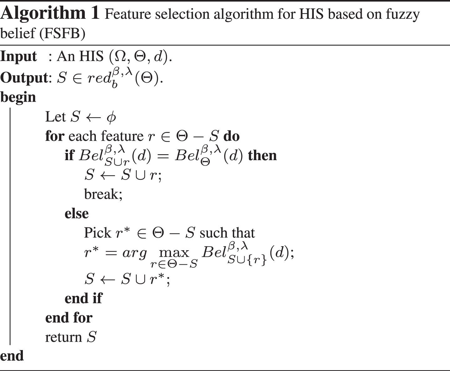
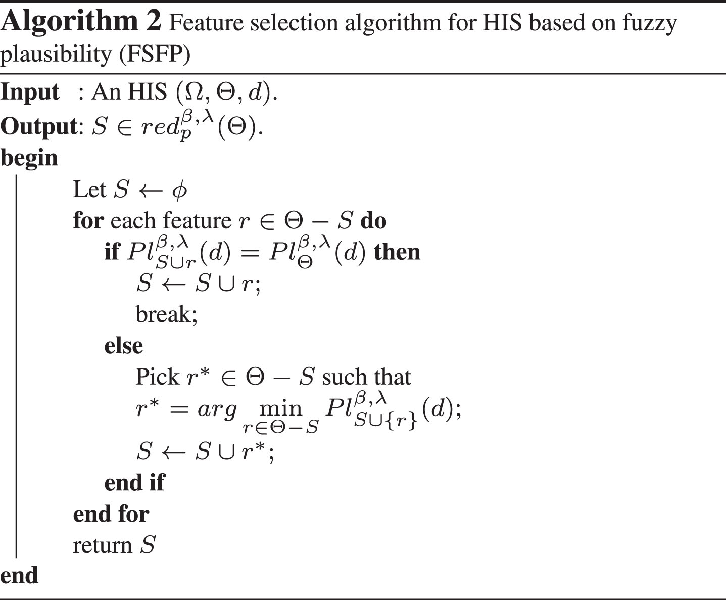
Algorithm 1 uses ${Bel}_{S}^{β, λ} (d)$ to select a feature that is added to the current candidate set in each loop. When ${Bel}_{S \cup r}^{β, λ} (d) = {Bel}_{Θ}^{β, λ} (d)$ , the algorithm terminates. The time complexity for computing ${Bel}_{S}^{β, λ} (d)$ is O (|S|) and the worst search time for a feature selection result requires (|Θ|+2) (|Θ|-1)/2 evaluations. So the overall time complexity of Algorithm 1 is O (|Θ|²|Ω|). The time complexity of Algorithm 2 is the same as that of Algorithm 1.

Example 4.15. (Continue with Example 3.4)

Taking β = 0.8 and λ = 0.2 as an example, the FSFB’s feature selection process for the data in Table 1 is demonstrated as follows.

${Bel}_{{θ_{1}, θ_{2}, θ_{3}}}^{β, λ} (d) = 0.81$ ,

${Bel}_{θ_{1}}^{β, λ} (d) = 0.50$ , ${Bel}_{θ_{2}}^{β, λ} (d) = 0$ , ${Bel}_{θ_{3}}^{β, λ} (d) = 0.75$ , ${Bel}_{{θ_{3}, θ_{1}}}^{β, λ} (d) = 0.81$ .

Therefore, {θ₃, θ₁} is a feature selection result of {θ₁, θ₂, θ₃}.

5 Experimental analysis and results

To evaluate the performance of FSFB, its classification performance and noise tolerance are compared with eight advanced feature selection algorithms on ten datasets. These datasets are downloaded from UCI Machine Learning Repository 1 , KRBM Dataset Repository 2 , and ASU feature selection repository 3 , and their details are listed in Table 2.

Table 2
10 datasets

NO. Datesets Abbr. Objects Features Classes

Total Numerical Nominal

1 Glass Gl 214 9 9 0 6

2 Insurance In 9822 85 43 42 2

3 Iris Ir 150 4 4 0 3

4 Lungharvard LH 32 12533 12533 0 2

5 Lungontario LO 39 2880 2880 0 2

6 PostateOutcome PO 26 12600 12600 0 2

7 Sonar So 208 60 60 0 2

8 Thyroid Th 7200 21 15 6 3

9 Wine Wi 178 13 13 0 3

10 Zoo Zo 101 16 1 15 7

NO.	Datesets	Abbr.	Objects	Features	Classes
1	Glass	Gl	214	9	9	0	6
2	Insurance	In	9822	85	43	42	2
3	Iris	Ir	150	4	4	0	3
4	Lungharvard	LH	32	12533	12533	0	2
5	Lungontario	LO	39	2880	2880	0	2
6	PostateOutcome	PO	26	12600	12600	0	2
7	Sonar	So	208	60	60	0	2
8	Thyroid	Th	7200	21	15	6	3
9	Wine	Wi	178	13	13	0	3
10	Zoo	Zo	101	16	1	15	7

5.1 Fuzzy belief and fuzzy plausibility

In this part, the anti-noise performance of fuzzy belief and fuzzy plausibility is verified.

The method of adding noise to data is as follows:

For real-valued attributes, first, transform the data to the interval [0,1], and then randomly select x% of the data to be randomly assigned a number between 0 and 1. x is taken as 0, 5, 10, 15, 20, and 25 respectively.

For categorical attributes, x% of randomly selected data are randomly assigned to the categorical attribute values. Similarly, x is taken as 0, 5, 10, 15, 20, and 25 respectively.

Parameters setting: β = 0.8, λ = 0.2.

Figures 1 and 2 show the fuzzy belief and fuzzy plausibility of 10 original data sets and their fuzzy belief and fuzzy plausibility after adding noise as the number of attributes in the data gradually increases. As the added noise continues to increase, the fuzzy belief and fuzzy plausibility do not change much, indicating that they are not sensitive to noise.

Fig. 1

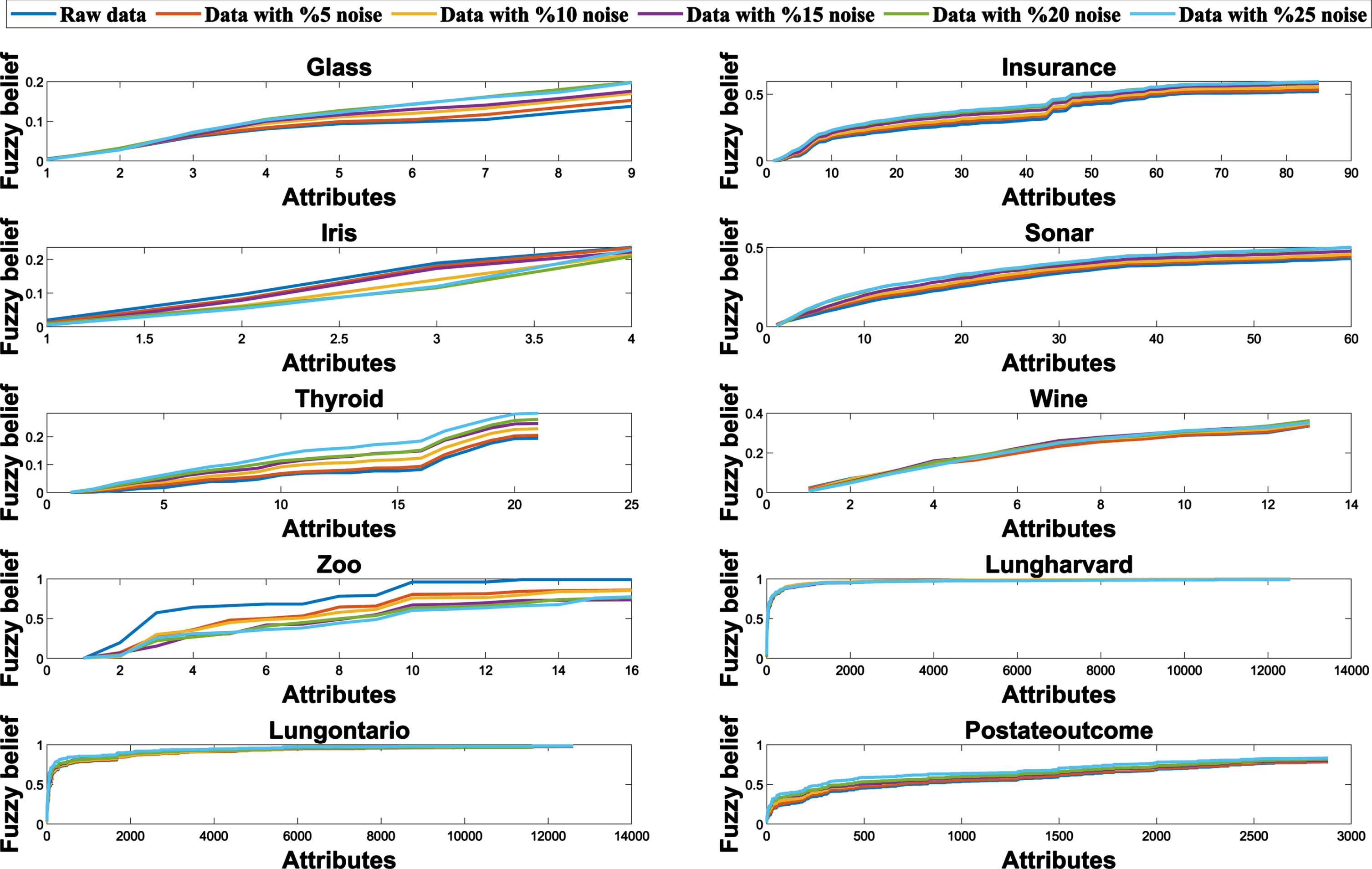
Fuzzy belief of different noise levels with the increase of attributes

Fig. 2

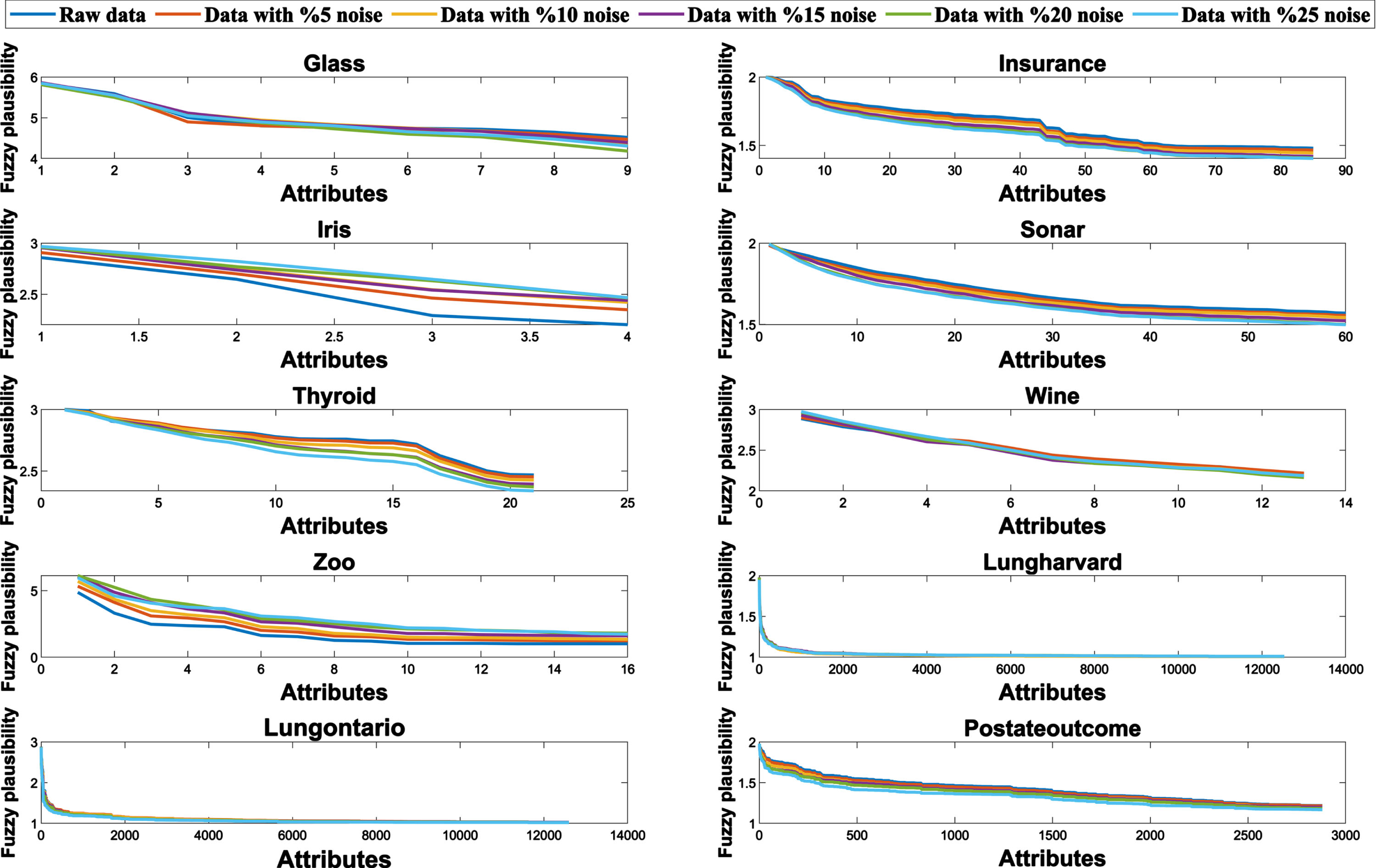
Fuzzy Plausibility of different noise levels with the increase of attributes

Figure 3 shows the mean and variance of fuzzy belief and fuzzy plausibility at different noise levels. When the noise level changes, the mean and variance of 9 data sets in 10 data sets almost remain unchanged, and those of Zoo have little change, as shown in Fig. 3. This indicates that noise has little effect on fuzzy belief and fuzzy plausibility.

Fig. 3

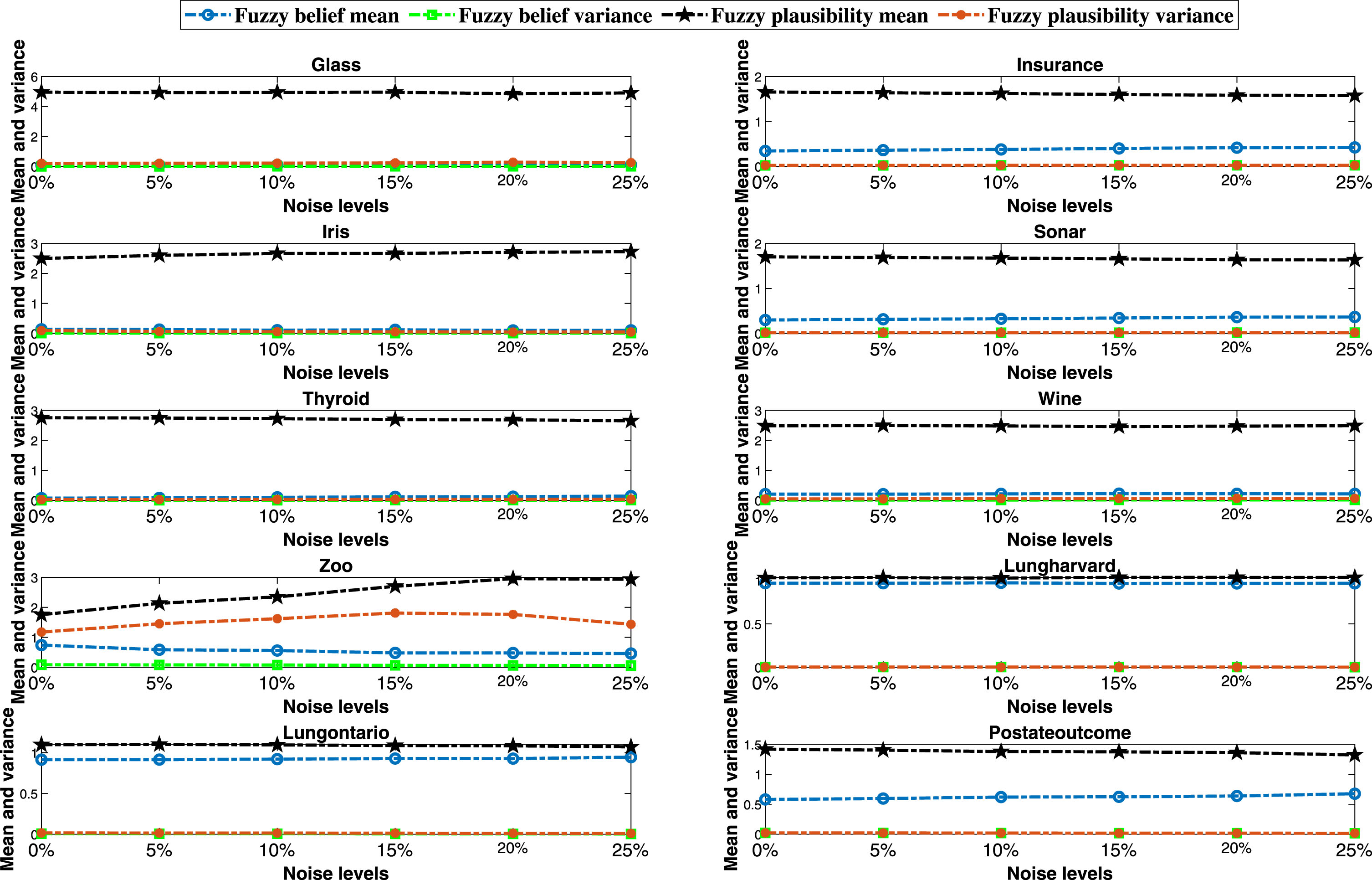
Mean and variance of fuzzy belief and fuzzy plausibility at different noise levels

Figure 4 shows that fuzzy belief and fuzzy plausibility are highly negatively correlated at various noise levels. Noise has little influence on the correlation between fuzzy belief and fuzzy plausibility. Therefore, only the performance of FSFB is shown below.

Fig. 4

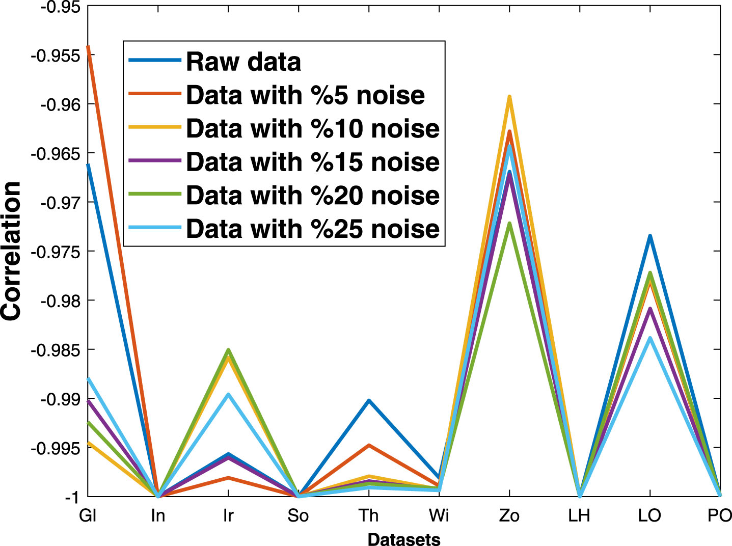
Correlation between fuzzy belief and fuzzy plausibility at different noise levels

5.2 Parameters analysis

Parameter values affect feature selection results. Let β and λ take values of {0.5, 0.6, 0.7, 0.8, 0.9} and {0.1, 0.2, 0.3, 0.4, 0.5}, respectively. Thus,β and λ have a total of 25 combinations. Each combination may correspond to a feature selection result of FSFB. The classification accuracy of all feature selection results on ten datasets is shown in Fig. 5 using the CART classifier.

Table 3 shows a pair of optimal parameter values for each dataset according to CART classifier.

The experimental results obtained by KNN are approximately consistent with CART.

Figure 5 shows that different values of parameters have a great impact on classification accuracy. Different values of parameter β mean different granularity. The larger the value of β, the more accurate the granularity is. The value of β can also be regarded as the threshold of information fusion. The larger the threshold is, the more accurate the information involved in the fusion is. Different values of parameter λ mean different anti-noise capabilities. The larger the value of λ is, the stronger the anti-noise capability is, but it also means that the risk of filtering out useful information will increase.

The following conclusions can be summarized from Fig. 5 and Table 3.

Within the value range of the two parameters, FSFB has achieved relatively high classification accuracy on most datasets, which shows that it has good stability.

For those datasets with a small number of samples, the value of λ is small, which means that if it is too large, key information may be filtered out.

For those datasets with a small number of features, the value of β is small, which means that they have low threshold requirements for information fusion because of few features.

For three large gene datasets, the value of β is large, which means that they have high threshold requirements for information fusion because of a large number of features. The fusion information needs to have a high degree of membership and thus characterizes the knowledge more accurately.

Fig. 5

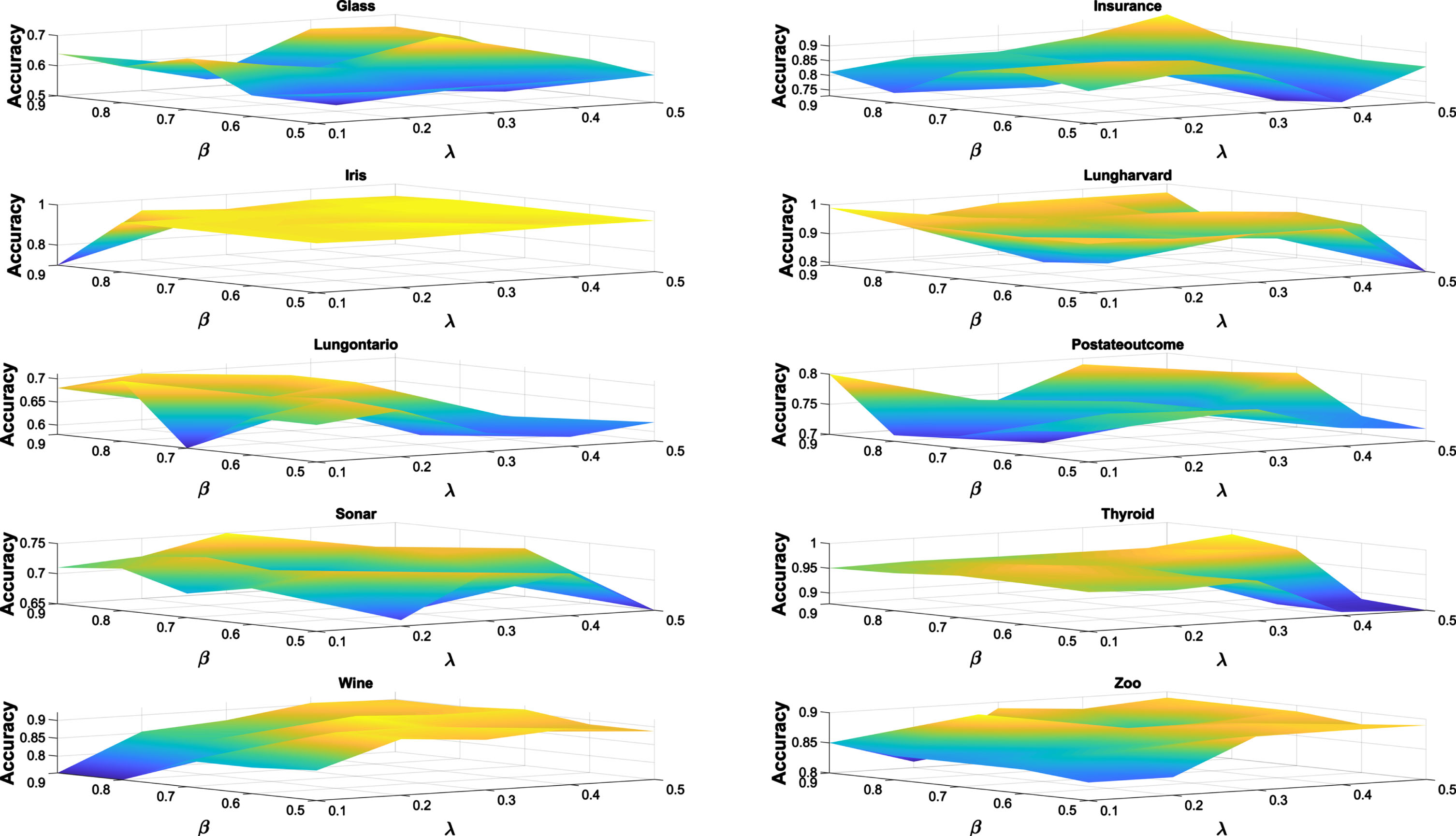
Classification accuracy of 10 datasets in the case of different parameter values by using CART classifier

Table 3

Optimal parameter values of ten datasets

NO.	Datesets	λ	β
1	Gl	0.4	0.7
2	In	0.5	0.9
3	Ir	0.3	0.6
4	LH	0.1	0.9
5	LO	0.1	0.8
6	PO	0.1	0.9
7	So	0.3	0.9
8	Th	0.5	0.8
9	Wi	0.3	0.7
10	Zo	0.2	0.8

5.3 Classification performance comparison

In this part, FSFB is compared with 7 state-of-the-art feature selection algorithms in classification performance and the size of selected feature subsets on 10 datasets. They are FBC [33], FSI [47], MFBC [31], NDI [46], NSI [48], VPDI [32], and QCISA-FS [55], respectively.

FBC is based on the fuzzy β-covering, and its fuzzy relation does not meet the reflexivity. FSI is based on fuzzy rough self-information, and its fuzzy relation meets the reflexivity. MFBC is based on the multi-granulation fuzzy rough sets, and its fuzzy relation does not meet the reflexivity. NDI is based on the neighborhood discrimination index, and its neighborhood relation meets the reflexivity. NSI is based on neighborhood self-information, and its neighborhood relation meets the reflexivity. VPDI is based on the variable precision discrimination index, and its fuzzy relation meets the reflexivity. FSFB is based on the fuzzy evidence theory and fuzzy β-covering, and its fuzzy relation meets the reflexivity. QCISA-FS is a quantum-inspired cooperative swarm intelligence algorithm based on the rough sets.

KNN (K-nearest neighbor,K=5) and CART (Classification And Regression Tree) are used to estimate the classification accuracy with the ten-fold cross-validation. All experimental results are the average of 100 repeated experiments. For those algorithms with parameters, their parameter values all take the optimal values. The final experimental data are shown in Tables 4–6.

Table 4
The number of selected features

Datasets Raw data FBC FSI MFBC NDI NSI VPDI QCISA-FS FSFB

Gl 9 5 3 6 6 4 6 3 4

In 85 10 5 18 8 5 6 4 5

Ir 4 2 1 2 2 1 2 1 2

LH 12533 15 6 24 15 5 9 6 9

LO 2880 13 73 32 19 21 17 16 13

PO 12600 6 2 18 9 5 7 7 5

So 60 10 9 18 22 6 9 5 9

Th 21 5 3 5 4 2 3 2 3

Wi 13 4 3 9 6 3 4 3 5

Zo 16 8 5 7 9 4 5 5 5

Average 2822.1 7.8 11 13.9 10 5.6 6.8 5.2 6

Datasets	Raw data	FBC	FSI	MFBC	NDI	NSI	VPDI	QCISA-FS	FSFB
Gl	9	5	3	6	6	4	6	3	4
In	85	10	5	18	8	5	6	4	5
Ir	4	2	1	2	2	1	2	1	2
LH	12533	15	6	24	15	5	9	6	9
LO	2880	13	73	32	19	21	17	16	13
PO	12600	6	2	18	9	5	7	7	5
So	60	10	9	18	22	6	9	5	9
Th	21	5	3	5	4	2	3	2	3
Wi	13	4	3	9	6	3	4	3	5
Zo	16	8	5	7	9	4	5	5	5
Average	2822.1	7.8	11	13.9	10	5.6	6.8	5.2	6

Table 5

Classification accuracy of the feature sets selected by KNN (%)

Datasets	Raw data	FBC	FSI	MFBC	NDI	NSI	VPDI	QCISA-FS	FSFB
Gl	66.97±1.28	70.50±1.43	71.21±1.24	69.51±1.45	70.03±1.44	72.68±1.13	69.82±1.37	71.32±1.41	71.85±1.18
In	93.48±0.06	93.52±0.06	93.27±0.06	93.66±0.05	93.51±0.09	92.87±0.08	93.46±0.08	93.38±0.05	94.04±0.02
Ir	94.88±0.71	96.63±0.35	95.99±0.13	96.63±0.35	96.63±0.35	95.99±0.13	96.63±0.35	95.99±0.13	96.63±0.35
LH	87.16±3.29	100.0±0.00	92.76±2.91	100.0±0.00	100.0±0.00	93.55±2.47	100.0±0.00	95.68±1.04	100.0±0.00
LO	69.05±2.40	81.15±2.01	80.90±2.48	71.94±2.33	64.62±2.87	75.49±1.68	81.41±2.90	79.73±2.35	81.26±1.30
PO	68.12±1.84	76.85±2.56	79.54±2.38	76.73±2.21	94.42±1.92	66.69±5.22	73.85±1.55	76.60±2.52	77.15±2.61
So	81.85±1.11	82.42±1.11	76.76±1.29	82.35±1.18	85.14±1.26	83.12±1.00	79.58±1.19	80.76±1.05	82.83±1.05
Th	94.97±0.06	92.58±0.00	96.86±0.06	96.80±0.07	96.62±0.06	97.80±0.05	96.81±0.07	97.37±0.07	98.51±0.05
Wi	96.69±0.61	96.12±0.89	85.83±0.80	97.53±0.38	96.71±0.43	94.61±0.50	96.38±0.54	96.04±0.69	96.42±0.55
Zo	94.68±1.02	90.95±0.93	86.96±1.31	94.42±1.31	93.89±0.85	90.20±0.57	86.21±1.18	92.67±0.99	96.04±0.00
Average	84.79±1.24	88.07±0.93	86.01±1.27	87.96±0.93	89.16±0.93	86.30±1.28	87.42±0.92	87.95±1.03	89.47±0.71

Table 6

Classification accuracy of the feature subsets selected by CART (%)

Datasets	Raw data	FBC	FSI	MFBC	NDI	NSI	VPDI	QCISA-FS	FSFB
Gl	67.74±2.05	65.43±2.38	65.51±2.17	68.94±1.85	66.64±2.01	68.04±1.88	66.53±1.76	68.27±2.15	69.29±2.32
In	90.62±0.20	93.11±0.10	92.36±0.14	91.20±0.17	93.85±0.04	93.79±0.05	93.78±0.05	92.43±0.12	93.94±0.03
Ir	94.79±1.01	95.34±0.92	95.39±0.20	95.34±0.92	95.34±0.92	95.39±0.20	95.34±0.92	95.39±0.20	95.34±0.92
LH	78.88±4.83	94.25±1.15	91.73±1.39	93.66±1.41	91.31±1.64	92.28±1.55	93.71±1.37	95.94±1.93	99.72±1.00
LO	61.49±6.23	72.21±4.37	61.00±5.59	74.01±4.52	69.36±4.84	64.41±4.33	70.97±4.06	71.06±4.97	71.03±4.21
PO	40.12±5.58	67.69±5.10	70.85±4.61	61.12±5.70	77.31±5.53	79.69±3.05	71.85±5.57	79.22±2.61	80.69±3.46
So	71.73±2.61	78.32±2.24	69.29±2.35	75.59±2.11	75.34±2.48	72.25±2.25	75.55±2.16	75.12±2.14	75.69±1.81
Th	99.59±0.04	92.58±0.00	97.90±0.09	97.26±0.14	98.22±0.09	97.74±0.06	97.27±0.12	97.32±0.09	98.83±0.07
Wi	89.90±1.42	92.08±1.31	81.22±1.61	90.52±1.41	91.17±1.26	88.45±1.38	91.94±1.38	91.69±1.50	92.20±1.54
Zo	89.94±0.73	89.18±0.82	89.76±0.96	89.86±0.79	89.20±0.73	89.65±0.50	88.84±0.48	90.57±0.82	90.10±0.76
Average	78.48±2.47	84.02±1.84	81.50±1.91	83.75±1.90	84.77±1.95	84.17±1.53	84.58±1.79	85.70±1.65	86.68±1.61

Table 4 indicates that all seven algorithms effectively reduce redundant features, especially for three large-scale gene datasets. The average size of the selected feature subsets is far smaller than that of the original datasets. FSFB achieved a dimension reduction of 84.13% for seven UCI datasets and 99.90% for three large-scale gene datasets. The average of features selected by FSFB is only slightly greater than NSI, but FSFB has the highest classification accuracy. Therefore, FSFB is not easy to overfit and underfit. The average of features selected by MFBC is the largest, but MFBC’s average classification accuracy is not high, which indicates that MFBC is overfitting.

Tables 5 and 6 show that FSFB is superior to the other six algorithms and the original datasets in terms of average classification accuracy. In a total of 20 experiments, FSFB achieved the highest classification accuracy 11 times and is far more than other algorithms. These results show that the proposed algorithm is effective. Table 7 shows the feature subsets obtained by FSFB. The bold data represent the maximum classification accuracy.

Table 7

Feature subsets selected by FSFB

Datasets	The selected feature subsets
Gl	{1, 4, 2, 3}
In	{1, 2, 5, 65, 82}
Ir	{4, 3}
LH	{12114, 12186, 11485, 1246, 2549, 11015, 8005, 7765, 1612}
LO	{2245, 166, 954, 1347, 1902, 2322, 2660, 2781, 1551, 1762, 2399, 2687, 1918}
PO	{9301, 6530, 4139, 7083, 5357}
So	{30, 23, 12, 45, 17, 59, 20, 54, 10}
Th	{3, 17, 21}
Wi	{7, 1, 10, 13, 12}
Zo	{4, 10, 9, 13, 2}

Each raw dataset is regarded as an algorithm and FSFB is regarded as the control algorithm. Friedman [50] and Bonferroni-Dunn tests [51] are used for analyzing the statistical differences between the control algorithm and other comparison algorithms.

The Friedman test is defined as follows: $F_{F} = \frac{(d - 1) χ_{F}^{2}}{d (a - 1) - χ_{F}^{2}} \sim F_{α} (a - 1, (a - 1) (d - 1)),$ (5.1) where $χ_{F}^{2} = \frac{12 d}{a (a + 1)} \sum_{k = 1}^{a} r_{k}^{2} - 3 d (a + 1),$ r_k is the average ranking of the k-th (k = 1, 2, ⋯ , a) algorithm on all datasets and d represents the number of data sets.

F_0.1 (8, 72) =1.7571 according to F-distribution table when α = 0.1, a = 9 and d = 10. According to Formula (5.1), Tables 8 and 9, the value of F_F is equal to 2.7596 and 3.391 respectively. Obviously, they are both greater than 1.7571. Therefore, the performance of 8 algorithms is statistically different for the two classifiers.

Table 8

Classification accuracy ranking of eight algorithms according to KNN

Date sets	Raw data	FBC	FSI	MFBC	NDI	NSI	VPDI	QCISA-FS	FSFB
Gl	9	5	4	8	6	1	7	3	2
In	5	3	8	2	4	9	6	7	1
Ir	9	3	7	3	3	7	3	7	3
LH	9	1	8	2	3	7	4	6	5
LO	8	3	4	7	9	6	1	5	2
PO	8	4	2	5	1	9	7	6	3
So	6	4	9	5	1	2	8	7	3
Th	8	9	4	6	7	2	5	3	1
Wi	3	6	9	1	2	8	5	7	4
Zo	2	6	8	3	4	7	9	5	1
Average	6.7	4.4	6.3	4.2	4	5.8	5.5	5.6	2.5

Table 9

Classification accuracy ranking of eight algorithms according to CART

Date sets	Raw data	FBC	FSI	MFBC	NDI	NSI	VPDI	QCISA-FS	FSFB
Gl	5	9	8	2	6	4	7	3	1
In	9	5	7	8	2	3	4	6	1
Ir	9	6	2	6	6	2	6	2	6
LH	9	3	7	5	8	6	4	2	1
LO	8	2	9	1	6	7	5	3	4
PO	9	7	6	8	4	2	5	3	1
So	8	1	9	3	5	7	4	6	2
Th	1	9	4	8	3	5	7	6	2
Wi	7	2	9	6	5	8	3	4	1
Zo	3	8	5	4	7	6	9	1	2
Average	6.8	5.2	6.6	5.1	5.2	5	5.4	3.6	2.1

Next, the Bonferroni-Dunn test [52] is used as a post hoc test to analyze the performance difference between the control algorithm and the comparison algorithms. Its critical value is defined as follows: ${CD}_{α} = q_{α} \sqrt{\frac{a (a + 1)}{6 d}},$ (5.2)

q_0.1 = 2.498 when α = 0.1 and a = 9 [52]. Therefore, CD_0.1 = 3 according to Formula (5.2) when α = 0.1, a = 9 and d = 10. The CD diagrams of the KNN classifier and CART classifier are shown in Figs. 6 and 7, respectively. Figure 6 shows that FSFB is statistically superior to VPDI, QCISA-FS, NSI, FSI, and the raw dataset at a confidence level of α = 0.1. Figure 7 shows that FSFB is statistically superior to MFBC, FBC, FSI, NDI, VPDI, and the raw dataset at a confidence level of α = 0.1.

Fig. 6

CD diagram of Bonferroni-Dunn test using KNN classifier

Fig. 7

CD diagram of Bonferroni-Dunn test using CART classifier

5.4 Robustness evaluation of seven feature selection algorithms

In this section, the noise tolerance performance of seven feature selection algorithms is evaluated.

In many practical applications, it is required for the feature selection algorithm to be robust, i.e., it can obtain a stable feature subset when exposed to data noise. If the selected feature subset varies significantly when exposed to data noise, this algorithm is said to be conditionally sensitive.

The robustness (stability) of the feature selection algorithm can be evaluated based on its ability to repeatedly select features when different batches of data with the same distribution are provided. As the true distribution of data is usually unknown, data from different batches are generated by adding different levels of noise.

Let Θ_j and Θ₀ denote the feature subsets selected by the jth batch of noisy data and the raw data, respectively. Then, the similarity between Θ_j and Θ₀ can be defined by Jaccard Index [54] as follows:

$T_{j} = | \frac{Θ_{j} ⋂ Θ_{0}}{Θ_{j} ⋃ Θ_{0}} | .$ (5.3)

T_j can provide an evaluation of the robustness and reflect the anti-noise ability of a feature selection algorithm. The greater the similarity, the stronger the anti-noise ability.

According to the method mentioned in section 6.1, 5%, 10%, 15%, 20% and 25% noises are added to the original data respectively. The experimental result is the average value of 10 times of noise added randomly.

Figure 8 and Table 10 show the average similarity of different algorithms and data sets. Compared with the UCI datasets, the large-scale gene datasets are more affected by noise because of too few samples. FSFB achieves the maximum similarity on six data sets in ten data sets, far more than other algorithms. While the proportion of noise increases, both the distribution of data and the importance of features will change. This leads to obvious differences in the best feature subset selected by the algorithm. Even so, the average similarity of FSFB still reaches 65%, at least 6% higher than other algorithms. Therefore, FSFB is more robust than the other six algorithms.

Fig. 8

Average similarity between feature subset obtained from original data and feature subsets obtained from noisy data

Table 10

Average similarity between feature subset obtained from original data and feature subsets obtained from noisy data

Datasets	FBC	FSI	MFBC	NDI	NSI	VPDI	QCISA-FS	FSFB
Gl	0.55±0.19	0.62±0.17	0.57±0.12	0.68±0.11	0.36±0.08	0.68±0.17	0.58±0.17	0.63±0.15
In	0.61±0.18	0.58±0.21	0.54±0.17	0.64±0.18	0.45±0.10	0.64±0.17	0.54±0.19	0.69±0.17
Ir	0.77±0.11	0.81±0.10	0.65±0.09	0.74±0.09	0.80±0.09	0.98±0.03	0.79±0.27	0.97±0.04
LH	0.57±0.23	0.55±0.24	0.24±0.20	0.54±0.20	0.44±0.20	0.60±0.21	0.46±0.17	0.63±0.20
LO	0.28±0.27	0.25±0.27	0.22±0.32	0.32±0.29	0.46±0.29	0.24±0.29	0.26±0.29	0.49±0.27
PO	0.18±0.27	0.19±0.28	0.21±0.28	0.26±0.28	0.16±0.26	0.23±0.30	0.20±0.31	0.33±0.30
So	0.68±0.15	0.65±0.18	0.66±0.18	0.70±0.18	0.62±0.14	0.67±0.19	0.56±0.23	0.63±0.20
Th	0.61±0.16	0.62±0.19	0.61±0.14	0.67±0.15	0.54±0.08	0.65±0.16	0.55±0.15	0.72±0.18
Wi	0.62±0.22	0.58±0.18	0.72±0.18	0.68±0.20	0.53±0.14	0.63±0.15	0.50±0.15	0.71±0.15
Zo	0.62±0.21	0.56±0.20	0.60±0.18	0.62±0.22	0.48±0.13	0.61±0.17	0.58±0.22	0.71±0.20
Average	0.55±0.20	0.54±0.20	0.50±0.19	0.59±0.19	0.48±0.15	0.59±0.18	0.50±0.22	0.65±0.19

6 Discussion and conclusion

This paper presents a novel distance metric that is guided by decision attributes and is more accurate than Euclidean distance for measuring the difference between nominal feature values. We establish a connection between fuzzy evidence theory and fuzzy β covering with an anti-noise mechanism, which addresses the computational challenges of fuzzy belief and fuzzy plausibility calculations. We propose two feature selection algorithms that are based on this new distance metric, fuzzy β covering, fuzzy evidence theory, and the anti-noise mechanism. Experimental results demonstrate that the proposed algorithms outperform six state-of-the-art algorithms in terms of classification performance and noise tolerance. Therefore, the algorithms proposed in this study are robust and effective. However, it should be noted that the computational complexity of the proposed algorithms is high, and grid optimization of parameters is required. This can result in long computational times when applied to large-scale gene datasets. In the future, we plan to investigate means of reducing computational complexity and automating parameter optimization of the proposed algorithms.

Acknowledgements

The authors would like to thank the editors and the anonymous reviewers for their valuable comments and suggestions, which have helped immensely in improving the quality of the paper. This work is supported by Excellent Scientific Research and Innovation Team of Anhui Colleges (2022AH010098), Doctoral Research Start Project of Chizhou University (CZ2021YJRC01), Provincial Quality Engineering Project of Higher Education Institutions (2022zybj068), Outstanding Engineer in Data Science and Big Data Technology, “Six Excellence and One Top” Project and Major Scientific Research Project of Higher Education Institutions in Anhui Province.

Appendix

1 . Proof of Theorem 3.8.

Proof. (1) It is obvious.

(2) 1)“ ${\underline{apr}}_{P}^{β, λ} (ϒ) \subseteq {\bar{apr}}_{P}^{β, λ} (ϒ)$ ” is proved in Theorem 3.1 of [33].

2) In order to prove that “ $λ \leq β \Rightarrow {\underline{apr}}_{P}^{β, λ} (ϒ) \subseteq ϒ$ ”, it is sufficient to show that $ϒ (ω) \geq 1 - β \Rightarrow {\underline{apr}}_{P}^{β, λ} (ϒ) (ω) \leq ϒ (ω) (ω \in Ω) .$

Let λ ≤ β, ϒ (ω) ≥1 - β . Put $A (ω) = {ω^{'} \in Ω : [ω]_{P}^{β} (ω^{'}) \geq λ}, B (ω) = Ω - A (ω) .$

Since λ ≤ β, we have $[ω]_{P}^{β} (ω) \geq β \geq λ$ . So ω ∈ A (ω).

Note that ϒ (ω) ≥1 - β. Then

$\begin{matrix} {\underline{apr}}_{P}^{β, λ} (ϒ) (ω) \\ = ⋀_{ω^{'} \in Ω} {(1 - [ω]_{P}^{β, λ} (ω^{'})) \lor ϒ (ω^{'})} \\ = (⋀_{ω^{'} \in A (ω)} {(1 - [ω]_{P}^{β, λ} (ω^{'})) \lor ϒ (ω^{'})}) ⋀ \\ (⋀_{ω^{'} \in B (ω)} {(1 - [ω]_{P}^{β, λ} (ω^{'})) \lor ϒ (ω^{'})}) \\ = (⋀_{ω^{'} \in A (ω)} {(1 - [ω]_{P}^{β} (ω^{'})) \lor ϒ (ω^{'})}) ⋀ \\ (⋀_{ω^{'} \in B (ω)} {(1 - 0) \lor ϒ (ω^{'})}) \\ = ⋀_{ω^{'} \in A (ω)} {(1 - [ω]_{P}^{β} (ω^{'})) \lor ϒ (ω^{'})} \\ \leq (1 - [ω]_{P}^{β} (ω)) \lor ϒ (ω) \\ \leq (1 - β) \lor ϒ (ω) = ϒ (ω) . \end{matrix}$

3) In order to prove that “ $β \geq λ \Rightarrow ϒ \subseteq {\bar{apr}}_{P}^{β, λ} (ϒ)$ , it is sufficient to show that $ϒ (ω) \leq β \Rightarrow ϒ (ω) \leq {\bar{apr}}_{P}^{β, λ} (ϒ) (ω) .$

Note that ϒ (ω) ≤ β. Then $\begin{matrix} {\bar{apr}}_{P}^{β, λ} (ϒ) (ω) & = ⋁_{ω^{'} \in Ω} {_{P}^{β, λ} (ω^{'}) \land ϒ (ω^{'})} \\ = (⋁_{ω^{'} \in A (ω)} {[ω]_{P}^{β, λ} (ω^{'}) \land ϒ (ω^{'})}) ⋁ \\ (⋁_{ω^{'} \in B ((ω))} {[ω]_{P}^{β, λ} (ω^{'}) \land ϒ (ω^{'})}) \\ = (⋁_{ω^{'} \in A (ω)} {[ω]_{P}^{β} (ω^{'}) \land ϒ (ω^{'})}) ⋁ \\ (⋁_{o^{'} \in B (ω)} (0 \land ϒ (ω^{'}))) \\ = ⋁_{ω^{'} \in A (ω)} {[ω]_{P}^{β} (ω^{'}) \land ϒ (ω^{'})} \\ \geq [ω]_{P}^{β} (ω) \land ϒ (ω) \\ \geq β \land ϒ (ω) \\ = ϒ (ω) . \end{matrix}$

(3) Let ϒ ⊆ Ξ. Then ∀ ω ∈ Ω, ϒ (ω) ≤ Ξ (ω).

In order to prove that ${\underline{apr}}_{P}^{β, λ} (ϒ) \subseteq {\underline{apr}}_{P}^{β, λ} (Ξ)$ and ${\underline{apr}}_{P}^{β, λ} (ϒ) \subseteq {\underline{apr}}_{P}^{β, λ} (Ξ)$ , it is sufficient to show that $ϒ (ω) \geq 1 - β \Rightarrow {\underline{apr}}_{P}^{β, λ} (ϒ) (ω) \leq {\underline{apr}}_{P}^{β, λ} (Ξ) (ω),$ $Ξ (ω) \leq β \Rightarrow {\bar{apr}}_{P}^{β, λ} (ϒ) (ω) \leq {\bar{apr}}_{P}^{β, λ} (Ξ) (ω) .$

Suppose ϒ (ω) ≥1 - β. Then $\begin{matrix} {\underline{apr}}_{P}^{β, λ} (ϒ) (ω) = ⋀_{ω^{'} \in Ω} {(1 - [ω]_{P}^{β, λ} (ω^{'}) \lor ϒ (ω^{'})} \\ \leq ⋀_{ω^{'} \in Ω} {(1 - [ω]_{P}^{β, λ} (ω^{'}) \lor Ξ (ω^{'})} = {\underline{apr}}_{P}^{β, λ} (Ξ) (ω) . \end{matrix}$

Suppose Ξ (ω) ≤ β. Then $\begin{matrix} {\bar{apr}}_{P}^{β, λ} (ϒ) (ω) = ⋁_{ω^{'} \in Ω} {[ω]_{P}^{β, λ} (ω^{'}) \land ϒ (ω^{'})} \\ \leq ⋁_{ω^{'} \in Ω} {[ω]_{P}^{β, λ} (ω^{'}) \land Ξ (ω^{'})} = {\bar{apr}}_{P}^{β, λ} (Ξ) (ω) . \end{matrix}$

(4) It follows from Proposition 2.6(1).

(5) It can be proved by Proposition 2.6(2).

(6) It can be proved by Proposition 2.6(2).

(7) It is sufficient to show that $\begin{matrix} (ϒ \cap Ξ) (ω) \geq 1 - β \Rightarrow \\ ({\underline{apr}}_{P}^{β, λ} (ϒ) \cap {\underline{apr}}_{P}^{β, λ} (Ξ)) (ω) \\ = ({\underline{apr}}_{P}^{β, λ} (ϒ \cap Ξ)) (ω), \end{matrix}$ $\begin{matrix} ϒ (ω), Ξ (ω) \leq β \Rightarrow ({\bar{apr}}_{P}^{β, λ} (ϒ \cup Ξ)) (ω) \\ = ({\bar{apr}}_{P}^{β, λ} (ϒ) \cup {\bar{apr}}_{P}^{β, λ} (Ξ)) (ω) . \end{matrix}$

Suppose (ϒ ∩ Ξ) (ω) ≥1 - β. Then ϒ (ω) , Ξ (ω) ≥1 - β. Thus

${\underline{apr}}_{P}^{β, λ} (ϒ) (ω) = ⋀_{ω^{'} \in Ω} {(1 - [ω]_{P}^{β, λ} (ω^{'})) \lor ϒ (ω^{'})},$ ${\underline{apr}}_{P}^{β, λ} (Ξ) (ω) = ⋀_{ω^{'} \in Ω} {(1 - [ω]_{P}^{β, λ} (ω^{'})) \lor Ξ (ω^{'})},$

${\underline{apr}}_{P}^{β, λ} (ϒ \cap Ξ) (ω) = ⋀_{ω^{'} \in Ω} {(1 - [ω]_{P}^{β, λ} (ω^{'})) \lor (ϒ \cap Ξ) (ω^{'})} .$

Hence $\begin{matrix} ({\underline{apr}}_{P}^{β, λ} (ϒ \cap Ξ)) (ω) \\ = ⋀_{ω^{'} \in Ω} {(1 - [ω]_{P}^{β, λ} (ω^{'})) \lor (ϒ (ω^{'}) \land (Ξ) (ω^{'}))} \\ = ⋀_{ω^{'} \in Ω} {(1 - [ω]_{P}^{β, λ} (ω^{'})) \lor ϒ (ω^{'})) \land \\ (1 - [ω]_{P}^{β, λ} (ω^{'})) \lor Ξ (ω^{'}))} \\ = (⋀_{ω^{'} \in Ω} {(1 - [ω]_{P}^{β, λ} (ω^{'})) \lor ϒ (ω^{'})}) ⋀ \\ (⋀_{ω^{'} \in Ω} {(1 - [ω]_{P}^{β, λ} (ω^{'})) \lor Ξ (ω^{'})}) \\ = {\underline{apr}}_{P}^{β, λ} (ϒ) (ω) ⋀ {\underline{apr}}_{P}^{β, λ} (Ξ) (ω) \\ = ({\underline{apr}}_{P}^{β, λ} (ϒ) \cap {\underline{apr}}_{P}^{β, λ} (Ξ)) (ω) . \end{matrix}$

Suppose ϒ (ω) , Ξ (ω) ≤ β. Then (ϒ ∪ Ξ) (ω) ≤ β. Thus

Thus

${\bar{apr}}_{P}^{β, λ} (ϒ) (ω) = ⋁_{ω^{'} \in Ω} {[ω]_{P}^{β, λ} (ω^{'}) \land ϒ (ω^{'})}$ ,

${\bar{apr}}_{P}^{β, λ} (Ξ) (ω) = ⋁_{ω^{'} \in Ω} {[ω]_{P}^{β, λ} (ω^{'}) \land Ξ (ω^{'})}$ ,

${\bar{apr}}_{P}^{β, λ} (ϒ \cup Ξ) (ω) = ⋁_{ω^{'} \in Ω} {[ω]_{P}^{β, λ} (ω^{'}) \land (ϒ \cup Ξ) (ω^{'})}$ .

Hence $\begin{matrix} ({\bar{apr}}_{P}^{β, λ} (ϒ \cup Ξ)) (ω) \\ = ⋁_{ω^{'} \in Ω} {[ω]_{P}^{β, λ} (ω^{'}) \land (ϒ (ω^{'}) \lor (Ξ) (ω^{'}))} \\ = ⋁_{ω^{'} \in Ω} {([ω]_{P}^{β, λ} (ω^{'}) \land ϒ (ω^{'})) \lor ([ω]_{P}^{β, λ} (ω^{'}) \land Ξ (ω^{'}))} \\ = (⋁_{ω^{'} \in Ω} {[ω]_{P}^{β, λ} (ω^{'}) \land ϒ (ω^{'})}) ⋁ \\ (⋁_{ω^{'} \in Ω} {[ω]_{P}^{β, λ} (ω^{'}) \land Ξ (ω^{'})}) \\ = {\bar{apr}}_{P}^{β, λ} (ϒ) (ω) ⋁ {\bar{apr}}_{P}^{β, λ} (Ξ) (ω) \\ = ({\bar{apr}}_{P}^{β, λ} (ϒ) \cup {\bar{apr}}_{P}^{β, λ} (Ξ)) (ω) . \end{matrix}$

(8) Obviously, $(\bar{1} - ϒ) (ω) \geq 1 - β \Leftrightarrow ϒ (ω) \leq β,$ $(\bar{1} - ϒ) (ω) < 1 - β \Leftrightarrow ϒ (ω) > β .$

Suppose $(\bar{1} - ϒ) (ω) < 1 - β$ . Then ${\underline{apr}}_{P}^{β, λ} (\bar{1} - ϒ) (ω) = 0$ , ${\bar{apr}}_{P}^{β, λ} (ϒ) (ω) = 1$ . Thus ${\underline{apr}}_{P}^{β, λ} (\bar{1} - ϒ) (ω) = (\bar{1} - {\bar{apr}}_{P}^{β, λ} (ϒ)) (ω) .$

Suppose $(\bar{1} - ϒ) (ω) \geq 1 - β$ . Then $\begin{matrix} {\underline{apr}}_{P}^{β, λ} (\bar{1} - ϒ) (ω) \\ = ⋀_{ω^{'} \in Ω} {(1 - [ω]_{P}^{β, λ} (ω^{'})) \lor ((\bar{1} - ϒ) (ω^{'}))} \\ = ⋀_{ω^{'} \in Ω} {(1 - [ω]_{P}^{β, λ} (ω^{'})) \lor (1 - ϒ (ω^{'}))} \\ = ⋀_{ω^{'} \in Ω} (1 - [ω]_{P}^{β, λ} (ω^{'}) \land ϒ (ω^{'})) \\ = 1 - ⋁_{ω^{'} \in Ω} ([ω]_{P}^{β, λ} (ω^{'}) \land ϒ (ω^{'})) \\ = 1 - {\bar{apr}}_{P}^{β, λ} (ϒ) (ω) \\ = (\bar{1} - {\bar{apr}}_{P}^{β, λ} (ϒ)) (ω) . \end{matrix}$

Thus ${\underline{apr}}_{P}^{β, λ} (\bar{1} - ϒ) = \bar{1} - {\bar{apr}}_{P}^{β, λ} (ϒ)$ .

Similarly, it can be proved that ${\bar{apr}}_{P}^{β, λ} (\bar{1} - ϒ) = \bar{1} - {\underline{apr}}_{P}^{β, λ} (ϒ)$ .□

2 . Proof of Proposition 5.7.

Proof. (1) ⇒ (2). Let $B \in {co}_{b}^{β, λ} (Θ)$ . Then $\forall i, {Bel}_{B}^{β, λ} (D_{i}^{λ}) = {Bel}_{Θ}^{β, λ} (D_{i}^{λ}) .$

So $\forall i, | {\underline{apr}}_{▵_{B}}^{β, λ} (D_{i}^{λ}) | = | {\underline{apr}}_{▵_{Θ}}^{β, λ} (D_{i}^{λ}) | .$

Since B ⊆ Θ, by Theorem 2.8(3), $\forall i, {\underline{apr}}_{▵_{B}}^{β, λ} (D_{i}^{λ}) \subseteq {\underline{apr}}_{▵_{Θ}}^{β, λ} (D_{i}^{λ}) .$

By Lemma 4.7, we have $\forall i, {\underline{apr}}_{▵_{B}}^{β, λ} (D_{i}^{λ}) = {\underline{apr}}_{▵_{Θ}}^{β, λ} (D_{i}^{λ}) .$

(2) ⇒ (3). Suppose ∀ i, ${\underline{apr}}_{▵_{B}}^{β, λ} (D_{i}^{λ}) = {\underline{apr}}_{▵_{Θ}}^{β, λ} (D_{i}^{λ})$ . Then $\forall i, {Bel}_{B}^{β, λ} (D_{i}^{λ}) = {Bel}_{Θ}^{β, λ} (D_{i}^{λ}) .$

This implies that $\sum_{i = 1}^{r} {Bel}_{B}^{β, λ} (D_{i}^{λ}) = \sum_{i = 1}^{r} {Bel}_{Θ}^{β, λ} (D_{i}^{λ}) .$

Thus ${Bel}_{B}^{β, λ} (d) = {Bel}_{Θ}^{β, λ} (d) .$

(3) ⇒ (1). Suppose ${Bel}_{B}^{β, λ} (d) = {Bel}_{Θ}^{β, λ} (d) .$ Then $\sum_{i = 1}^{r} \frac{| {\underline{apr}}_{▵_{B}}^{β, λ} (D_{i}^{λ}) |}{n} = \sum_{i = 1}^{r} \frac{| {\underline{apr}}_{▵_{Θ}}^{β, λ} (D_{i}^{λ}) |}{n} .$

Thus $\sum_{i = 1}^{r} (| {\underline{apr}}_{▵_{Θ}}^{β, λ} (D_{i}^{λ}) | - | {\underline{apr}}_{▵_{B}}^{β, λ} (D_{i}^{λ}) |) = 0 .$

Since B ⊆ Θ, by Theorem 2.8(3), we have ${\underline{apr}}_{▵_{B}}^{β, λ} (D_{i}^{λ}) \subseteq {\underline{apr}}_{▵_{Θ}}^{β, λ} (D_{i}^{λ})$ .

Then $\forall i, | {\underline{apr}}_{▵_{Θ}}^{β, λ} (D_{i}^{λ}) | - | {\underline{apr}}_{▵_{B}}^{β, λ} (D_{i}^{λ}) | \geq 0 .$

This implies that $\forall i, | {\underline{apr}}_{▵_{Θ}}^{β, λ} (D_{i}^{λ}) | = | {\underline{apr}}_{▵_{B}}^{β, λ} (D_{i}^{λ}) | .$

By Lemma 4.7, we have $\forall i, {\underline{apr}}_{▵_{B}}^{β, λ} (D_{i}^{λ}) = {\underline{apr}}_{▵_{Θ}}^{β, λ} (D_{i}^{λ}) .$

Thus $B \in {co}_{b}^{β, λ} (Θ)$ .□

3 . Proof of Proposition 5.9.

Proof. (1) ⇒ (2). Let $B \in {co}_{p}^{β, λ} (Θ)$ . Then $\forall i, {Pl}_{B}^{β, λ} (D_{i}^{λ}) = {Pl}_{Θ}^{β, λ} (D_{i}^{λ}) .$

So $\forall i, | {\bar{apr}}_{▵_{B}}^{β, λ} (D_{i}^{λ}) | = | {\bar{apr}}_{▵_{Θ}}^{β, λ} (D_{i}^{λ}) | .$

Since B ⊆ Θ, by Theorem 2.8(3), $\forall i, {\bar{apr}}_{▵_{Θ}}^{β, λ} (D_{i}^{λ}) \subseteq {\bar{apr}}_{▵_{B}}^{β, λ} (D_{i}^{λ}) .$

By Lemma 4.7, we have $\forall i, {\bar{apr}}_{▵_{B}}^{β, λ} (D_{i}^{λ}) = {\bar{apr}}_{▵_{Θ}}^{β, λ} (D_{i}^{λ}) .$

(2) ⇒ (3). Suppose ∀ i, ${\bar{apr}}_{▵_{B}}^{β, λ} (D_{i}^{λ}) = {\bar{apr}}_{▵_{Θ}}^{β, λ} (D_{i}^{λ})$ . Then $\forall i, {Pl}_{B}^{β, λ} (D_{i}^{λ}) = {Pl}_{Θ}^{β, λ} (D_{i}^{λ}) .$

This implies that $\sum_{i = 1}^{r} {Pl}_{B}^{β, λ} (D_{i}^{λ}) = \sum_{i = 1}^{r} {Pl}_{Θ}^{β, λ} (D_{i}^{λ}) .$

Thus ${Pl}_{B}^{β, λ} (d) = {Pl}_{Θ}^{β, λ} (d) .$

(3) ⇒ (1). Suppose ${Pl}_{B}^{β, λ} (d) = {Pl}_{Θ}^{β, λ} (d) .$ Then $\sum_{i = 1}^{r} \frac{| {\bar{apr}}_{▵_{B}}^{β, λ} (D_{i}^{λ}) |}{n} = \sum_{i = 1}^{r} \frac{| {\bar{apr}}_{▵_{Θ}}^{β, λ} (D_{i}^{λ}) |}{n} .$

Thus $\sum_{i = 1}^{r} (| {\bar{apr}}_{▵_{B}}^{β, λ} (D_{i}^{λ}) | - | {\bar{apr}}_{▵_{Θ}}^{β, λ} (D_{i}^{λ}) |) = 0 .$

Since B ⊆ Θ, by Theorem 2.8(3), we have ${\bar{apr}}_{▵_{Θ}}^{β, λ} (D_{i}^{λ}) \subseteq {\bar{apr}}_{▵_{B}}^{β, λ} (D_{i}^{λ})$ .

Then $\forall i, | {\bar{apr}}_{▵_{B}}^{β, λ} (D_{i}^{λ}) | - | {\bar{apr}}_{▵_{Θ}}^{β, λ} (D_{i}^{λ}) | \geq 0 .$

This implies that $\forall i, | {\bar{apr}}_{▵_{B}}^{β, λ} (D_{i}^{λ}) | = | {\bar{apr}}_{▵_{Θ}}^{β, λ} (D_{i}^{λ}) | .$

By Lemma 4.7, we have $\forall i, {\bar{apr}}_{▵_{B}}^{β, λ} (D_{i}^{λ}) = {\bar{apr}}_{▵_{Θ}}^{β, λ} (D_{i}^{λ}) .$

Thus $B \in {co}_{p}^{β, λ} (Θ)$ .□

Footnotes

http://archive.ics.uci.edu/ml/index.php

http://leo.ugr.es/elvira/DBCRepository/

http://featureselection.asu.edu/datasets.php

References

Zhou

, Li

, Zhao

and Wu

, Feature interaction for streamingfeature selection, IEEE Transactions on Neural Networks andLearning Systems 32(10) (2021), 4691–4702.

Pawlak

, Rough sets, International Journal of Computer andInformation Science 11(5) (1982), 341–356.

Qian

, Liang

, Pedrycz

and Dang

, Positive approximation:an accelerator for attribute reduction in rough set theory, Artificial Intelligence 174(10) (2010), 597–618.

Lynn

, Restrepo

, Cornelis

and Gomez

, Neighborhoodoperators for covering-based rough sets, Information Sciences 336 (2016), 21–44.

Dubois

and Prade

, Rough fuzzy sets and fuzzy rough sets, International Journal of General Systems 17(3) (2007), 191–209.

, Yu

, Liu

and Wu

, Neighborhood rough set basedheterogeneous feature subset selection, Information Sciences 178(18) (2008), 3577–3594.

Zhang

, Qu

and Li

, Attribute reduction based on D-S evidencetheory in a hybrid information system, International Journal ofApproximate Reasoning 148 (2022), 202–234.

Wang

, Chen

and Dong

, Attribute reduction via localconditional entropy, International Journal of Machine Learningand Cybernetics 10(12) (2019), 3619–3634.

Wang

, Huang

, Shao

and Chen

, Uncertainty measures forgeneral fuzzy relations, Fuzzy Sets and Systems 360(2019), 82–96.

10.

Sun

, Wang

, Ding

, Qian

and Xu

, Feature selection usingfuzzy neighborhood entropy-based uncertainty measures for fuzzyneighborhood multigranulation rough sets, IEEE Transactions onFuzzy Systems 29(1) (2021), 19–33.

11.

Wang

, Huang

, Shao

and Fan

, Fuzzy rough set-basedattribute reduction using distance measures, Knowledge-BasedSystems 164 (2019), 205–212.

12.

, Zhang

, Zhou

and Pedrycz

, Large-scale multimodalityattribute reduction with multi-kernel fuzzy rough sets, IEEETransactions on Fuzzy Systems 26(1) (2018), 226–238.

13.

Wang

, Wang

, Shao

, Qian

and Chen

, Fuzzy roughattribute reduction for categorical data, IEEE Transactions onFuzzy Systems 28 (2020), 818–830.

14.

Zeng

, Li

, Liu

, Zhang

and Chen

, A fuzzy rough setapproach for incremental feature selection on hybrid informationsystems, Fuzzy Sets and Systems 258 (2015), 39–60.

15.

Zhang

, Chen

, Zhang

, Li

, Chen

and Wen

, Newuncertainty measurement for categorical data based on fuzzyinformation structures: an application in attribute reduction, Information Sciences 580 (2021), 541–577.

16.

Jiang

, Liu

, Garg

and Zhang

, Large group decision-makingbased on interval rough integrated cloud model, AdvancedEngineering Informatics 56 (2023), 101964.

17.

Al-shami

T.M.

, An improvement of rough sets’ accuracy measure usingcontainment neighborhoods with a medical application, Information Sciences 569 (2021), 110–124.

18.

Al-shami

T.M.

, Topological approach to generate new rough setmodels, Complex Intelligent Systems 8 (2022), 4101–4113.

19.

Al-Shami

T.M.

, Improvement of the approximations and accuracymeasure of a rough set using somewhere dense sets, SoftComputing 25 (2021), 14449–14460.

20.

Al-shami

T.M.

Maximal rough neighborhoods with a medical application, Journal of Ambient Intelligence and Humanized Computing (2022), https://doi.org/10.1007/s12652-022-03858-1.

21.

Al-shami

T.M.

and Mhemdi

, Approximation spaces inspired by subsetrough neighborhoods with applications, DemonstratioMathematica 56 (2023), 20220223.

22.

Chen

, Li

, Zhang

and Kwong

, Evidence-theory-basednumerical algorithms of attribute reduction withneighborhood-covering rough sets, International Journal ofApproximate Reasoning 55(3) (2014), 908–923.

23.

, Huang

, Liu

, Xie

and Zhang

, Information structuresin a covering information system, Information Sciences 507 (2020), 449–471.

24.

Han

, Covering rough set structures for a locally finite coveringapproximation space, Information Sciences 480 (2019), 420–437.

25.

, Leung

and Zhang

, Generalized fuzzy rough approximationoperators based on fuzzy coverings, International Journal ofApproximate Reasoning 48(3) (2008), 836–856.

26.

Feng

, Zhang

and Mi

, The reduction and fusion of fuzzycovering systems based on the evidence theory, InternationalJournal of Approximate Reasoning 53(1) (2012), 87–103.

27.

Yang

and Hu

, Fuzzy neighborhood operators and derived fuzzycoverings, Fuzzy Sets and Systems 370 (2019), 1–33.

28.

Deer

, Cornelis

and Godo

, Fuzzy neighborhood operators basedon fuzzy coverings, Fuzzy Sets and Systems 312 (2017), 17–35.

29.

, Couple fuzzy covering rough set models and theirgeneralizations to CCD lattices, International Journal ofApproximate Reasoning 126 (2020), 48–69.

30.

Zhang

, Zhan

, Wu

and Alcantud

, Fuzzy β-coveringbased (I, T)-fuzzy rough set models and applications tomulti-attribute decision-making, Computers and IndustrialEngineering 128 (2019), 605–621.

31.

Huang

, Li

and Qian

, Noise-tolerantfuzzy-β-covering-based multigranulation rough sets and featuresubset selection, IEEE Transactions on Fuzzy Systems 30(7) (2022), 2721–2735.

32.

Huang

, Li

Noise-tolerant discrimination indexes for fuzzy γ covering and feature subset selection, IEEE Transactions on Neural Networks and Learning Systems (2022), doi: 10.1109/TNNLS.2022.3175922.

33.

Huang

and Li

, A fitting model for attribute reduction withfuzzy β-covering, Fuzzy Sets and Systems 413(2021), 114–137.

34.

Dempster

, Upper and lower probabilities induced by a multivaluedmapping, Annals of Mathematical Statistics 38(2) (1967), 325–339.

35.

Lin

, Liang

and Qian

, An information fusion approach bycombining multigranulation rough sets and evidence theory, Information Sciences 314 (2015), 184–199.

36.

Chen

, Li

, Zhang

and Kwong

, Evidence theory basednumerical algorithms of attribute reduction with neighborhoodcovering rough sets, International Journal of ApproximateReasoning 55(3) (2014), 908–923.

37.

Peng

and Zhang

, Feature selection for interval-valued databased on D-S evidence theory, IEEE Access 9 (2021), 122754–122765.

38.

Zhan

, Wang

, Ding

, Yao

Three-way behavioral decision making with hesitant fuzzy information systems: survey and challenges, IEEE/CAA Journal of Automatica Sinica (2022), Doi: 10.1109/JAS.2022.106061.

39.

Xue

, Deng

and Garg

, Uncertain database retrieval withmeasure-Based belief function attribute values under intuitionisticfuzzy set, Information Sciences 546 (2021), 436–447.

40.

Kaushal

, Garg

and Lohani

, Global intuitionistic fuzzyweighted C-ordered means clustering algorithm, InformationSciences 642 (2023), 119087.

41.

, Garg

and Deng

, A new uncertainty measure of discreteZ-numbers, Intnational Journal of Fuzzy Systtems 22(2020), 760–776.

42.

, Leung

and Mi

, On generalized fuzzy belief functions ininfinite spaces, IEEE Transactions on Fuzzy Systems 17(2) (2009), 385–397.

43.

Yao

, Mi

and Li

, Attribute reduction based on generalizedfuzzy evidence theory in fuzzy decision systems, Fuzzy Sets andSystems 170(1) (2011), 64–75.

44.

Tao

, Zhang

and Mi

, The reduction and fusion of fuzzycovering systems based on the evidence theory, InternationalJournal of Approximate Reasoning 53(1) (2012), 87–103.

45.

, Hu

and Wang

, Probability granular distance-based fuzzyrough set model, Applied Soft Computing 102(5) (2021), 107064: 1–13.

46.

Wang

, Hu

, Wang

, Chen

, Qian

and Dong

, Featureselection based on neighborhood discrimination index, IEEETransactions on Neural Networks and Learning Systems 29(7) (2018), 2986–2999.

47.

Wang

, Huang

, Ding

and Cao

, Attribute reduction withfuzzy rough self-information measures, Information Sciences 549 (2021), 68–86.

48.

Wang

, Huang

, Shao

, Hu

and Chen

, Feature selectionbased on neighborhood self-information, IEEE Transactions onCybernetics 50(9) (2020), 4031–4042.

49.

, Zhang

, Wang

, Liu

, Song

and Wen

, Gene selectionin a single cell gene space based on D-S evidence theory, Interdisciplinary Sciences: Computational Life Sciences 14(3) (2022), 722–744.

50.

Friedman

, A comparison of alternative tests of significance forthe problem of m rankings, The Annals of MathematicalStatistics 11(1) (1940), 86–92.

51.

Demsar

, Statistical comparison of classifiers over multiple datasets, Journal of Machine Learning Research 7(1) (2006), 1–30.

52.

Dunn

, Multiple comparisons among means, Journal of theAmerican Statistical Association 56(293) (1961), 52–64.

53.

Yang

and Mao

, Robust feature selection for microarray databased on multicriterion fusion, IEEE/ACM Transactions onComputational Biology and Bioinformatics 8(4) (2011), 1080–1092.

54.

Kalousis

, Prados

and Hilario

, Stability of featureselection algorithms: A study on high-dimensional spaces, Knowledge and Information Systems 12(1) (2007), 95–116.

55.

Zouache

and Abdelaziz

F.B.

, A cooperative swarm intelligencealgorithm based on quantum-inspired and rough sets for featureselection, Computers and Industrial Engineering 115(2018), 26–36.

Feature selection for hybrid information systems based on fuzzy β covering and fuzzy evidence theory

Abstract

Keywords

1 Introduction

1.1 Research background and related works

1.2 Motivation and inspiration

1.3 Organization

2 Preliminaries

Table 1 An HIS (Ω, Θ, d) Ω Headache (θ1) Muscle pain (θ2) Temperature (θ3) Symptom (d) ω1 No No 36 Health ω2 No * * Health ω3 * No 37 Health ω4 Middle * 39 Flu ω5 Sick Yes 39.5 Flu ω6 * No 40 Flu ω7 Middle * 37.5 Reinitis ω8 Middle Yes * Reinitis

4.1 Fuzzy belief function and fuzzy plausibility function

4.2 λ-belief reduction and λ-plausibility reduction in an HIS

5 Experimental analysis and results

Acknowledgements

Appendix

Footnotes

References

Table 1
An HIS (Ω, Θ, d)

Ω Headache (θ₁) Muscle pain (θ₂) Temperature (θ₃) Symptom (d)

ω₁ No No 36 Health

ω₂ No * * Health

ω₃ * No 37 Health

ω₄ Middle * 39 Flu

ω₅ Sick Yes 39.5 Flu

ω₆ * No 40 Flu

ω₇ Middle * 37.5 Reinitis

ω₈ Middle Yes * Reinitis