Multi scale encoder-decoder network with Time Frequency Attention and S-TCN for single channel speech enhancement

Abstract

The goal of speech enhancement is to restore clean speech in noisy environments. Acoustic scenarios with low signal-to-noise ratios (SNR) make it quite challenging to extract the target speech from its noise. In the current study, to enhance noisy speech, we propose a feature recalibration based multi-scale convolutional encoder-decoder architecture with squeeze temporal convolutional networks (S-TCN) bottleneck. Each multi-scale convolutional layer in encoder and decoder is followed by time-frequency attention module (TFA). The recalibration based multi-scale 2D convolution layers are used to extract local and contextual information. Additionally, the recalibration network is equipped with a gating mechanism to control the flow of information among the layers, enabling weighting of the scaled features for noise suppression and speech retention. The fully connected layer (FC) in the bottleneck part of encoder-decoder contains a few neurons, which capture the global information from the multi-scale 2D convolution layer and reduce parameters. A S-TCN, inspired by the popular temporal convolutional neural network (TCNN), is inserted between the encoder and the decoder to model long-term dependencies in speech. The TFA is a highly efficient network component, that operates through two simultaneous attentions, one focused on time frames, and the other on frequency channels. These attentions work together to explicitly exploit positional information to create a two-dimensional attention map to effectively capture the significant time-frequency distribution of speech. Utilizing the common voice dataset, our proposed model consistently enhances results compared to the current benchmarks, as demonstrated by two extensively utilized objective measures PESQ and STOI. The proposed model shows significant improvements, with average PESQ and STOI scores increasing by 45.7% and 23.8% respectively for seen background noises, and by 43.5% and 21.4% for unseen background noises, when compared to the quality of noisy speech. Tests validate that the proposed approach outperforms numerous cutting-edge algorithms.

Keywords

TFA - time-frequency attention S-TCN - squeeze temporal convolutional networks MSCL - multi scale convolutional layer FR - feature recalibration FRMSC - feature recalibration based multi scale convolution

1 Introduction

An approach to denoise speech [22] consists of removing background noise and preserving good perceptual quality and intelligibility. Since audio calls, teleconferencing, speech recognition, and hearing aids use the technology, the technology has been studied for decades. A noise spectrum estimate is required to determine what clean speech looks like given the additive noise assumption, using traditional signal processing methods like spectral subtraction [2] and Wiener filtering [20]. These models work well in the presence of stationary noise. However, nonstationary, and structured noises, such as dogs barking, babies crying, or traffic horns, may not generalize well. Later NMF based models are used to deal with nonstationary noises [12]. A neural network has been used for speech enhancement since the 1980s [32]. DNNs (Deep neural networks) are often used when computation power increases, for example, [23, 50]. The models based on DNN for speech enhancement have attained top-of-the-line results in the past few years. The DNNs are generally trained in supervised environments, where they learn to predict the clean speech from the noisy speech. These methods can be categorized as time-frequency domain methods and waveform domain methods. It is well known that a large body of research uses time-frequency representation [38, 50]. To modulate clean speech, these methods use a complex spectrum (e.g., Ideal Ratio Mask [47]) as input. After that, a resynthesized waveform is constructed from the extracted spectral features in the input noisy speech and phase of noisy speech. From a noisy waveform input, another family of speech enhancement models [11 , 33] predicts the clean waveform directly. Both WaveNet [29] and U-Net [36] are popular SE architectures.

In addition, convolutional neural networks (CNN) have been exploited in a number of approaches, for example, in [18] where a convolution encoder-decoder (CED) was employed to approximate the mapping relationship among corrupted speech and desired speech signals. To enhance the learning of multi-resolution features, an advanced approach is implemented using a multi-resolution convolutional auto-encoders (MCARE) model [27]. The MCARE model incorporates dilated convolutions to expand the network’s receptive fields within the Wavenet architecture. Additionally, a gated mechanism is employed to regulate the flow of information among different layers [34]. These improvements contribute to the overall performance of the system.

In addition, the gated recurrent network (GRN) technique is integrated with dilated 2D convolution layers to effectively expand the receptive field within the time-frequency (T-F) domain [44]. This combination enables the model to capture larger contextual information and enhances its ability to process T-F representations. A combination of recurrent and convolution frameworks has been employed to progress enhancement performance even further. In the convolution recurrent network (CRN) [45], for example, the encoder-decoder (CED) is combined with the long-term interaction model (LSTM), with the CED capturing local T-F patterns, and the LSTM capturing long-term dependencies. As compared to LSTM, CRN performed better. In the study described in [49], a multiscale encoder is introduced, which leverages a temporal convolution module (TCM) to capture relevant speech features. TCM is useful for learning the long-term dependencies of the past. For further improving enhanced quality additional bottleneck layers are added between the encoder and decoder. Among them are dilated convolutions [39], TCN [15, 30], and LSTMs [5].

In recent research, various attention mechanisms have been integrated into speech enhancement techniques to enhance their effectiveness. The role of attention mechanisms has been a subject of exploration by researchers in the past few years [6 , 54]. The self-attention (SA) approach [37] is an effective framework for aggregating context within the input sequence. In [31], a comprehensive CNN framework was put forth for handling SE within the temporal domain. This model incorporated self-attention within both the encoder as well as decoder stages. Phan et al. proposed a SA methodology along with (de)convolution layers. This approach aimed to focus attention on the temporal context of speech within generators, leading to the development of SASEGAN [33]. In another work [53], researchers proposed an attention method that combines both time and frequency domain attentions. This technique was employed for tasks such as denoising and dereverberation, referred to as time-frequency attention.

Methods such as those listed above are promising and signify the current state of the art in this field. It does, however, have several limitations. It is common to use a fixed kernel size (filter) when using CED or CRN methods. A small kernel can be used to extract local information from the signal, while a larger kernel should be used to extract contextual information. There is a need for a method that is capable of extracting both local information and contextual information. Furthermore, LSTM implementations typically involve high computational loads. These computational loads can be challenging when the models are installed on devices with limited resources [4, 8]. Moreover, LSTMs require sequential processing, which can make training and inference slower, especially for long sequences such as audio signals in speech enhancement tasks [24, 25]. Despite this, the exploding and vanishing gradient problem and the difficulty of parallel training are some of their main drawbacks. For superior performance and less memory requirements, it would be desirable to use more efficient models such as temporal convolutional networks [1 , 30] instead of LSTM. Additionally, the Inception network [40] concatenates the features of different scales and assigns equal weight to them. In this scenario, features are considered equally important, which may pose problems when noise induces features. According to our work, features could be assigned different weights to improve this further.

Self-attention [31 , 53] calculates attention scores by evaluating the relationship between individual elements within the input sequence. This process leads to the creation of a dense attention matrix. However, as the length of the sequence grows, this computation becomes resource-intensive in terms of computation.

An encoder-decoder with skip connections and bottleneck layers is the basis for our model [36]. We refine the bottleneck representation by squeezed temporal convolutional layers [51]. The motivation behind this work is the achievement of effective multi-scale convolution and attention mechanisms.

A novel multi-scale convolutional architecture for speech enhancement is proposed, where each feature recalibration based multi-scale convolutional layer is followed by a TFA module and S-TCN in the bottleneck. This method overcomes the limitations of fixed kernel size used in traditional convolutional U-Net architectures. In proposed model by assigning a different weight to each feature in each scale, we can capture the interdependency between local and contextual information within the signal, thus retaining speech components while suppressing noise components. We are taking advantages of both the feature recalibration based multi-scale convolution and TFA modules. The advantage of feature recalibration based multi-scale convolution over traditional convolution with fixed kernel size is the extraction of local as well as contextual information.

The reason for using TFA over Self-attention [31 , 53] is that it calculates attention scores by evaluating the relationship between individual elements within the input sequence. This process leads to the creation of a dense attention matrix. However, as the length of the sequence grows, this computation becomes resource-intensive in terms of computation.

The TFA module comprises two parallel attentions: one for the time dimension (referred to as TA) and another for the frequency dimension (referred to as FA). These attentions generate two sets of 1-D attention maps. These maps serve as guidance for the models, helping them to focus on specific time frames (‘where’) and frequency-wise channels (‘what’). Following this, the TA and FA attentions are merged to produce a final 2D attention map. This map assigns distinct attention weights to individual time-frequency spectral components. As a result, the network can effectively capture the distribution of speech in the time-frequency representation. The bottleneck S-TCM blocks have the responsibility of handling the task of modeling temporal sequences. The tests have shown that the proposed model consistently enhances performance compared to the current benchmarks using two commonly used objective measures, such as PESQ and STOI.

Specific Contributions

To gain features of different scales, we first introduce the feature recalibration based multi-scale convolutional encoder-decoder module, which exploits kernels of different sizes in every convolutional layer to overcome the drawback of fixed kernel size used in traditional convolutional U-Net architectures. By assigning a different weight to each feature in each scale, it is possible to capture the interdependency between local and contextual information within the signal, thus retaining speech components while suppressing noise components.

The second step involves introducing bottleneck convolutional layers, which are 2D convolution layers with kernels of size (1,1) for compressing the information flow of the proposed model.

Third, in the bottleneck part of encoder-decoder a fully connected (FC) layer is used to decrease the size of encoder output and the S-TCN layer is used to model temporal sequences at different dilation rates of (1, 2, 4, 8, 16, 32).

Forth, the TFA module is introduced after every feature recalibration based multi-scale convolutional encoder-decoder layer. The TFA [52] is a highly efficient network component, that operates through two simultaneous attentions, one focused on time frames, and the other on frequency wise channels. These attentions work together to explicitly exploit positional information to create a two-dimensional attention map to effectively capture the significant time-frequency distribution of speech.

2 Model

2.1 Problem setting

In the time domain, a noisy speech signal can be expressed as follows: $x [t] = s [t] + n [t]$ (1) In Equation (1) s[t] is clean speech, n[t] is noise and x[t] is noisy speech with time index t.

By applying STFT on both sides of Equation (1) the T-F domain representation is given by $X_{t, f} = S_{t, f} + N_{t, f}$ (2)

In Equation (2) S_t,f is clean speech, X_t,f is the noisy mixture and N_t,f is noise. Where t ∈ {1, …, T} is time frame index and f ∈ {1, …, F} is frequency index.

The clean speech S_t,f and the noisy mixture X_t,f have been mapped employing a neural network model, and the mapping relation is configured by M. The estimation of the mapping function occurs through the optimization of the loss function, expressed as:

$\begin{matrix} Loss = \frac{1}{TF} \sum_{t = 1}^{T} \sum_{f = 1}^{F} {[M (| X_{t, f} |) - | S_{t, f} |]}^{2} \\ = \frac{1}{TF} \sum_{t = 1}^{T} \sum_{f = 1}^{F} {(| {\hat{S}}_{t, f} | - | S_{t, f} |)}^{2} \end{matrix}$ (3)

In Equation (3) |X_t,f| is the magnitude spectrum of the noisy speech signal and |S_t,f| is magnitude spectrum clean speech signal. Where t ∈ {1, …, T} is time frame index and f ∈ {1, …, F} is frequency index.where $| {\hat{S}}_{t, f} |$ is the predicted target speech’s magnitude, which is coupled with the phase of noisy mixture to recover the intended speech.

2.2 Proposed network architecture

The Fig. 1 depicts the proposed FRMSC-S-TCN-Net architecture. The proposed model takes the magnitude of the noisy speech as input and outputs the estimated magnitude of the target speech. The proposed model consists of an encoder, decoder, and bottleneck layer. The convolutional encoder consists of six convolutional layers, which include an input convolution layer, a bottleneck convolution layer, and four feature recalibration based multi-scale convolution layers. Each multi-scale convolution layer internally consists of five convolution blocks that have distinct kernel sizes 1×2, 3×3, 5×5, 7×7, 9×9 to extract multi-scale features in each layer of multi-scale convolutional encoder and decoder. By using convolutions with smaller kernel sizes, we can extract the features of short duration speech, thus capturing the local dependencies between adjacent T-F points. A kernel with a size of (1,2) is used to extract the feature from two adjacent T-F points. Feature extraction from long-duration speech is possible using convolutions with large kernel sizes. After extracting the features by using convolutions with different kernel sizes, the FR layer is introduced to allow the network to choose the features that are to be used selectively based on their weights. The TFA module is introduced after every feature recalibration based multi-scale convolutional encoder-decoder layer. The TFA is a highly efficient network component, that operates through two simultaneous attentions, one focused on time frames, and the other on frequency wise channels. These attentions work together to explicitly exploit positional information to create a two-dimensional attention map to effectively capture the significant time-frequency distribution of speech. The bottleneck convolution layer is an essential part of the architecture. It consists of a 2-D convolution layer having (1,1) kernels and 64 channels. This layer is positioned before the last layer of encoder and the first decoder layer, as depicted in Fig. 1. Its purpose is to decrease the dimensionality of the input. The convolution decoder shares a symmetric structure with the convolution encoder. The connecting layers receive the convolutional encoder’s output. The convolutional decoder obtains the information flow after it has been processed by the connection layers. To capture the long-term interdependency between the temporal frames, the proposed technique employs the connection layers. The dimension would inevitably expand if the multi-scaled convolutional sub-blocks were combined. Therefore, a method for keeping the information while also reducing the dimension and computational cost must be developed. In order to overcome this, we adopt a fully connected (FC) layer because its parameter count is lower than that of the RNN-based layer, resulting in a reduced dimension in the FC layer’s output compared to the encoder’s output. The fully connected (FC) layer is followed by S-TCN. In our model we used Squeeze TCN as connection layer. To achieve large temporal receptive field, we stack three groups of S-TCMs with a dilation rate exponentially increasing for each group (1, 2, 4, 8, 16, 32). Between the convolutional encoder and decoder, the skip connections are also introduced. The stride size of all layers is (1,2), except the multi-scale output layer, which has a fixed stride size (1,1). The number of channels in FRMSC layer of encoder and decoder are 32, 64, 128, 256. The number of channels in input and output 2D convolution are set to 16. The number of channels in output deconvolution layer is set to 1.

Fig. 1

The proposed FRMSC-S-TCN-Net architecture.

2.3 Feature recalibration based multi-scale convolutional layer (FRMSCL)

An area in which CNN can modify certain high-level features is known as the receptive field. Local information can be extracted from a small receptive field, while contextual information can be extracted from a large receptive field [44]. Traditionally, CNNs use a fixed kernel size, compromising local and contextual information. It is addressed by creating a feature recalibration based multi-scale convolutional layer (FRMSCL). This layer captures data at various scales and generates a multi-scaled feature. In FRMSCL, multiple convolution operations are included, which apply different sizes of kernels for capturing information at different scales. In the proposed model we used five parallel convolution operations with kernel sizes of 1×2, 3×3, 5×5, 7×7, and 9×9 to extract multi-scale features in each layer of multi scale convolutional encoder and decoder. By using convolutions with smaller kernel sizes, we can extract the features of short duration speech, thus capturing the local dependencies between adjacent T-F points. A kernel with a size of (1,2) is used to extract the feature from two adjacent T-F points. Feature extraction from long-duration speech is possible using convolutions with large kernel sizes. The features extracted by kernels with larger sizes contain more contextual information than smaller kernels. The batch-normalization and LeakyReLU [26] are used after each convolution. The output vectors of each convolution are then concatenated into one vector, which is used as the input vector for the next stage. A similar structure exists in multi-scale deconvolution layer, which replaces convolution operators with deconvolution operators. After extracting the features by using convolutions with different kernel sizes, the FR layer is introduced to allow the network to choose the features that are to be used selectively based on their weights. We call the proposed feature recalibration based multi-scale convolutional layer as FRMSC layer. Each FRMSCL is composed of m convolutions with same number of channels but different kernel sizes for capturing different features.

The input to the FRMSC layer is X, and K = k₁, k₂, …, k_m is the output, where k_m is captured by the m^th 2D convolution that has different kernel size compared with other 2D convolutions. In order to estimate the recalibration coefficients, two criteria can be employed: Using the recalibration coefficients, multi-scaled features extracted with different kernel sizes could be evaluated to assess the nonlinear relation, and speech components could be given relatively higher weights than noisy ones. These criteria are met by activating two FC layers, Sigmoid and ReLU. $\begin{matrix} c_{1 m} = w_{1 m} ⊙ k_{m} + b_{1 m} \end{matrix}$ (4) In Equation (4) c_1m is output of FC1, w_1m is weight corresponding to FC layer 1 (FC1) and b_1m is bias corresponding to FC layer 1 (FC1). Where k_m is captured by the m^th 2D convolution. $\begin{matrix} a_{m} = max [0, c_{1 m}] \end{matrix}$ (5) In Equation (5) a_m is output of ReLU and c_1m is output of FC1. $\begin{matrix} c_{2 m} = w_{2 m} ⊙ a_{m} + b_{2 m} \end{matrix}$ (6) In Equation (6) c_2m is output of FC2, w_2m is weight corresponding to FC layer 2 (FC2) and b_2m is bias corresponding to FC layer 2 (FC2). Where a_m is output of ReLU. $\begin{matrix} r s_{m} = \frac{e^{c_{2 m}}}{e^{c_{2 m + j}}} \end{matrix}$ (7) In Equation (7) The rs_m is a vector containing recalibration coefficients of m^th scaled feature. Where j = [1,1,…….1, 1,1,…….1] and e is operated on c_2m element wise. Where c_2m is output of FC2. In our application, we use the ReLU function as a non-negative constraint. The rs_m is a vector containing recalibration coefficients of m^th scaled feature. With Sigmoid, we introduce a gating function that assigns dissimilar weights to speech as well as noise components based on the success of the gating mechanism. The p_m is rescaled m^th feature and is given by $p_{m} = k_{m} ⊙ r s_{m}$ (8) In Equation (8) p_m is rescaled m^th feature, k_m is captured by the m^th 2D convolution and rs_m is a vector containing recalibration coefficients of m^th scaled feature.

We then introduced a skip connection [7] inside the FRMSC layer which does not introduce any parameters in additional. Finally, the output of FRMSC layer with residual connection and ReLU is given as $D = max [0, K + P]$ (9) In Equation (9) D is the final output of FRMSC layer with residual connection and ReLU, K is output of multi-scale convolution layer and P is the rescaled multi-scale feature.

By learning weights from multi-scale features, the proposed FRMSC-S-TCN-Net helps maintain speech components and suppress noise components in noisy mixtures after features are extracted from multi-scale features.

2.4 Time-frequency attention (TFA)

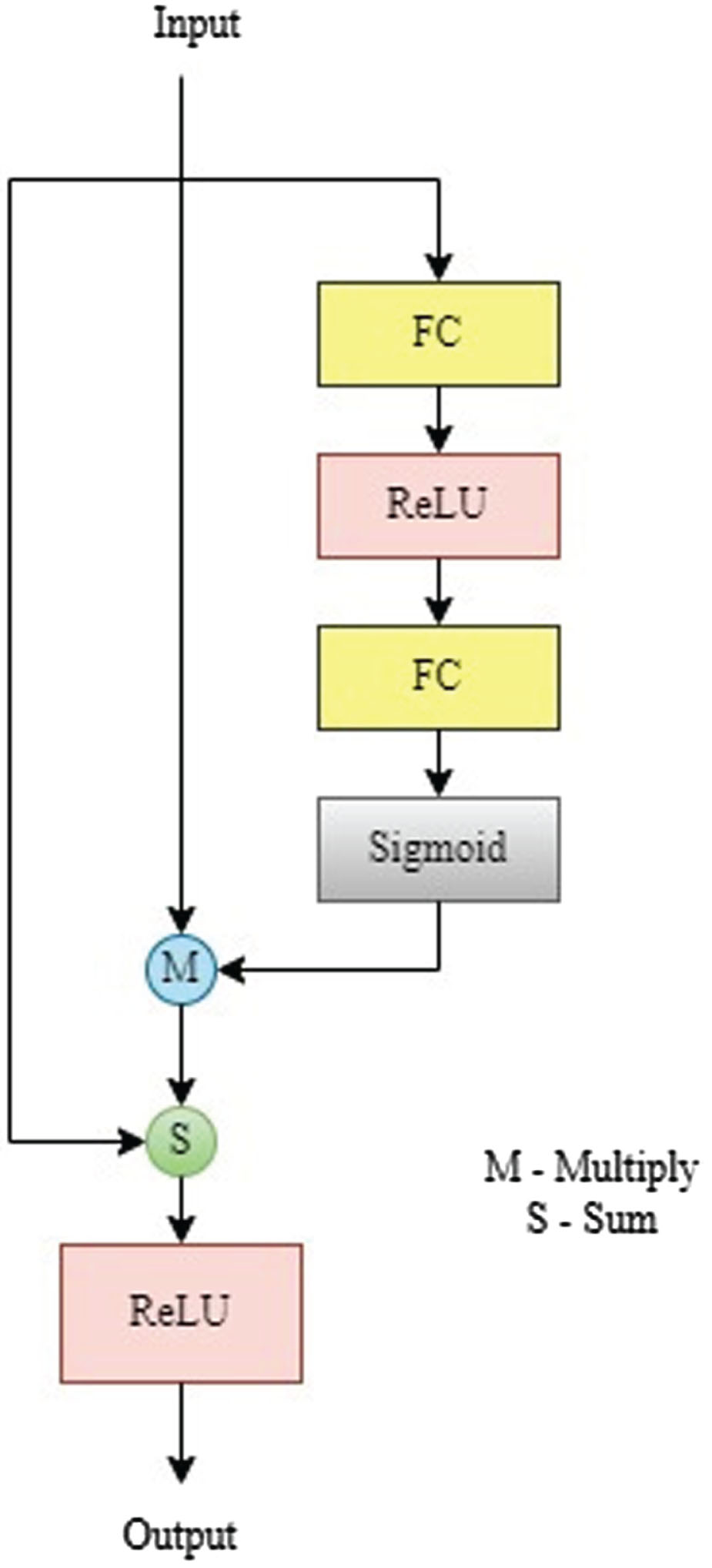
A TFA module serves as a computational component that accepts an intermediate input in the form of a spectrogram representation Y, where Y ∈ R^T×F. This input comprises T frames, each containing F frequency wise channels. The output is an improved representation $\hat{Y} \in R^{T \times F}$ , featuring distinct T-F attention characteristics. The TFA mechanism is presented in Fig. 3.

Fig. 2

recalibration layer.

Fig. 3

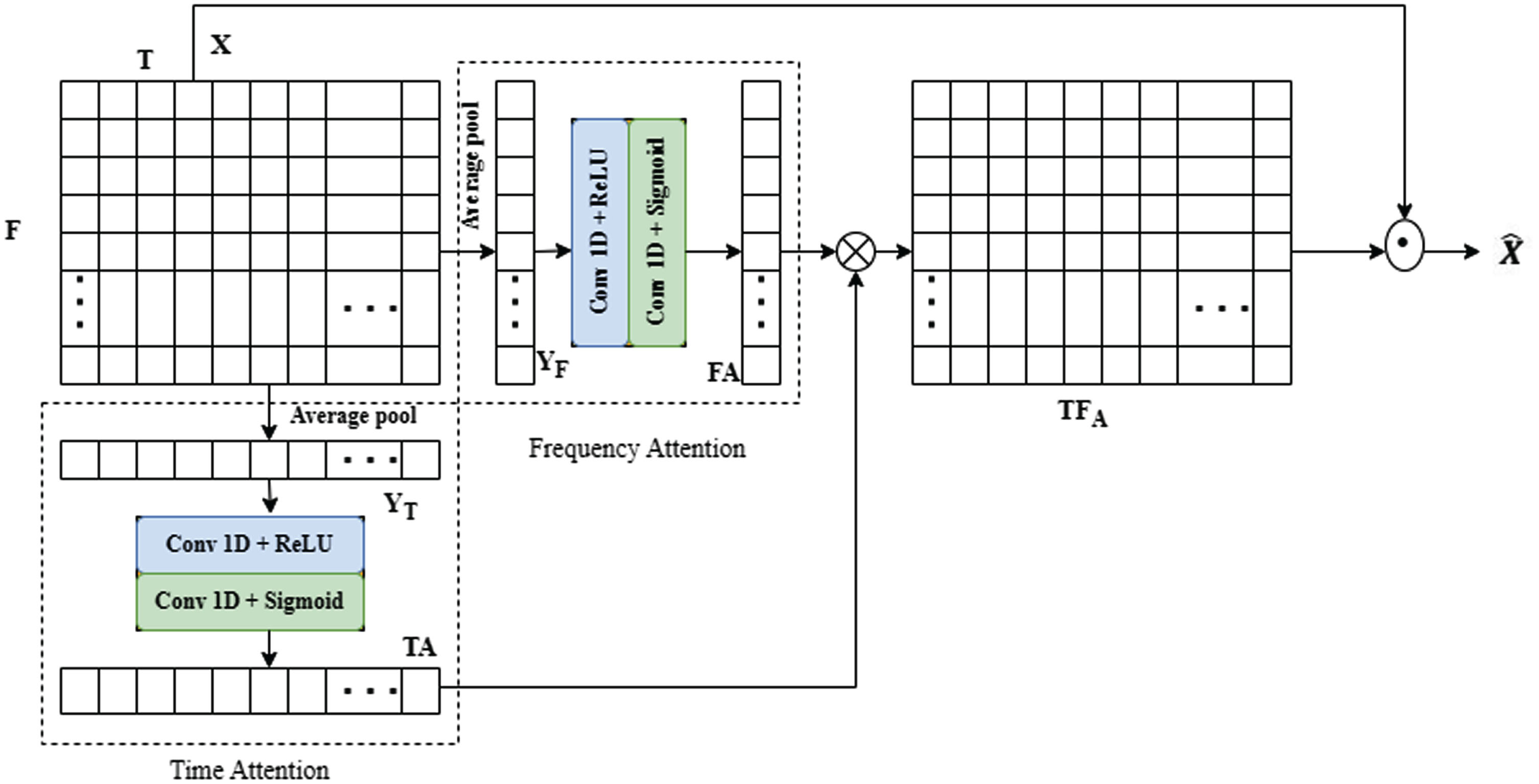
TFA module [52].

In TFA two simultaneous attentions referred to as TA and FA are used to generate a time-frame attention map (TA = R^1×T) and a frequency-dimension attention map (FA = R^F×1). Subsequently, these two 1-D attention maps are merged using a tensor multiplication process, leading to the creation of a 2-D T-F (time-frequency) attention map TFA = R^T×F, incorporating positional information. Each attention branch captures correlations through a two-step process:

Information Aggregation The TA and FA segments combine the complete information of the utterance across the time and frequency aspects, respectively. We utilize global average pooling, which generates comprehensive and generally applicable information descriptors for the complete utterance.

In particular, the TA branch performs global average pooling across the frequency axis on the provided input Y. This process produces time frame statistic M_T = R^1×T. $M_{T} (t) = \frac{1}{F} \sum_{f = 1}^{F} Y (t, f)$ (10) In Equation (10) t is time-frame index and f is discrete-frequency index. Y (t, f) is input of TFA module. Where M_T (t) is t^th element of M_T.

Similarly, the TA branch performs global average pooling across the time axis on the provided input Y. This process produce frequency statistic M_F = R^F×1. $M_{F} (f) = \frac{1}{T} \sum_{t = 1}^{T} Y (t, f)$ (11) In Equation (11) t is time-frame index and f is discrete-frequency index. Y (t, f) is input of TFA module. Where M_F (f) is f^th element of M_F.

Attention Generation: Frequently, a two-layer fully-connected (FC) layer is utilized for channel attention, as mentioned in [10, 48]. Nonetheless, incorporating FC layers results in a significant increase in parameters, which becomes particularly problematic for lengthy speech data. As an alternative, researchers have proposed a more efficient approach to achieve effective channel attention by employing 1-D convolution [46].

We utilize a pair of consecutive dilated 1-D convolutional layers for capturing relationships within the descriptors and acquiring a nonlinear correlation to generate the attention map. To be more precise, when provided with the descriptor M_T, the attention map within the TA branch is computed as follows:

$TA = σ ({Conv}_{2}^{TA} (ReLU ({Conv}_{1}^{TA} (M_{T}))))$ (12) In Equation (12) the Sigmoid activation is represented by σ and two dilated convolutions having dilation rates of 1,2 are represented by Conv.The M_T is the global average pooling across the frequency axis.

The FA branch utilizes the same method to create the frequency-wise attention map when provided with the descriptor M_F $FA = σ ({Conv}_{2}^{FA} (ReLU ({Conv}_{1}^{FA} (M_{F}))))$ (13) In Equation (13) the Sigmoid activation is represented by σ and two dilated convolutions having dilation rates of 1,2 are represented by Conv.The M_F is the global average pooling across the time axis.

Next, the attention maps derived from the two attention pathways combine through a tensor multiplication process ⊗, yielding our ultimate 2-D time-frequency attention map, referred to as TFA, which can be expressed as: $TFA = TA \otimes FA$ (14) In Equation (14) TA is the attention map generated by Time attention branch and FA is the attention map generated by frequency attention branch.

The (t, f) ^th element 2D attention is computed as: $TFA (t, f) = TA (t) \times FA (f)$ (15) In Equation (15) TA (t) is the attention map generated by time attention branch at time index t and FA (t) is the attention map generated by frequency attention branch at frequency index f.

Finally, TFA modules output is $\hat{Y} = Y ⊙ TFA$ (16) In Equation (16) ⊙ is element wise multiplication and Y is input of TFA module.

2.5 Bottleneck convolutions

One of the challenges faced in multi-scale convolutional layers is the need to address the issue of combining the multi-scale features. This process of concatenation can lead to an expansion in the feature dimensions, resulting in an increase in computational expenses. Hence, there is a requirement for a framework that can preserve the information while reducing dimensions. To address this, we incorporate bottleneck convolutional layers into the proposed architecture, as it has been proposed that a low-dimensional embedding could potentially encompass enough information about a sizable patch, according to previous techniques [41, 42]. The bottleneck convolution layer is an essential part of the architecture. It consists of a 2-D convolution layer having (1,1) kernels and 64 channels. Following the convolution layer, there is batch normalization and LeakyReLU activation function. This layer is positioned before the last layer of encoder and the first decoder layer, as depicted in Fig. 1. Its purpose is to decrease the dimensionality of the input.

2.6 Bottleneck layers between encoder-decoder (Connection Layers)

Long-term temporal information can be useful in improving speech, but the original convolutional encoder-decoder does not effectively use it [3, 45]. To capture the long-term interdependency between the temporal frames, the CRN technique employs the LSTM. A Squeeze TCN, inspired by the popular temporal convolutional neural network (TCNN), is inserted between the encoder and the decoder to model long-term dependencies in speech. The temporal convolutional module was initially proposed in [1]. The TCNs are computationally more efficient than LSTMs. TCNs can parallelize computations across time steps, while LSTMs are inherently sequential in nature. This parallelization allows TCNs to process input sequences faster, which can be especially beneficial for speech enhancement models that deal with long sequences. Also, TCNs have been shown to perform better than LSTMs in certain types of sequence modeling tasks, particularly those that involve long-term dependencies. This is because TCNs use dilated convolutions, which allows them to capture dependencies across long time scales. It is believed that TCN is a useful tool for long-range sequential modelling. The authors proposed repeatedly stacking TCNs that gradually widen the receptive field with increasing dilation rates perform well in the SE task [15, 55]. But because of the bottleneck’s abrupt dimension expansion, such a design is anticipated to have a high parameter burden. In order to overcome this problem, in [39] several enhancements are made in comparison to the original TCM and named as Squeezed TCN, which may reduce the number of parameters by roughly 72% over TCM while still achieving equivalent performance. The dimension would inevitably expand if the multi-scaled convolutional sub-blocks were combined. Therefore, a method for keeping the information while also reducing the dimension and computational cost must be developed. In order to overcome this, we adopt a fully connected (FC) layer because its parameter count is lower than that of the RNN-based layer, resulting in a reduced dimension in the FC layer’s output compared to the encoder’s output.

2.7 Multi-scale convolution based output layer

In Fig. 1, we incorporate a skip connection that connects the input of multi-scale output layer, as depicted in the lower part of the figure. Consequently, by leveraging the information flow from the previous decoder layer and the magnitude of the noisy speech input, the multi-scale output layer is capable of estimating the magnitude of the target speech. The multi-scale output layer consists of five 2-D deconvolutional layers with different kernel sizes. In contrast to the FRMSC layer, which concatenates varying scaled features, the multi-scale output layer sums the different scaled features to produce an output matrix of the same size as the input matrix. By doing so, the multi-scale output layer effectively incorporates both local as well as contextual information. The stride size of the output layer is set to (1,1) and it is followed by batch-normalization and linear activation.

3 Experiments

3.1 Datasets

Our system is tested using the Common Voice [28] dataset, a publicly accessible voice dataset sourced from volunteers worldwide. In order to train machine learning models, people can use this dataset to develop voice applications. A total of 1653880 (1.6 million) utterances from 84659 speakers are included in this dataset. For the training and validation sets, we randomly select 2000 and 400 utterances from the Common Voice corpus, respectively, from the English corpus. Overall, 400 utterances are included in the test set which are also taken from the Common Voice corpus. Our validation and training sets included 115 [9] different types of noises and varying signal SNR values of –5 dB to +10 dB. There are 50,000 training and 4,000 validation utterances made in each mixed procedure. The clean speech, noise, and SNRs are all selected at random. To determine the model’s generalization ability to various noises, we have created two test sets. one set with seen noises and the other with unseen noises. From NOIZEUS [21] database we have taken unseen noises, which include white, street, restaurant, and babble noises to prepare an unseen test set at SNR values of –5 dB to +10 dB.

3.2 Baselines and model setup

The FRMSC-S-TCN-Net employs a Short-Time Fourier Transform (STFT) with a Hanning window lasting 32 milliseconds, a filter duration of 32 milliseconds, and a hop interval of 16 milliseconds. To train the model, we utilized the common voice corpus, with 80 epochs on 4-second utterances. The model training was carried out using the Adam optimizer with a learning rate of 0.0001 [14]. The mean square error (MSE) is used as the objective function for both the baseline and proposed FRMSC-S-TCN-Net methods. The benchmark frameworks used for analysing the performance are a DNN [50], MRCAE [27], CRN [45], GRN [44], TCNN [30], DARCN [19], Dense U-Net [31], Clean U-Net[17] and SA U-Net[11].

3.3 Evaluation metrics

Two objective metrics are used to evaluate the enhancement performance of various models, including perceptual evaluation of speech quality (PESQ) [35] and short-time objective intelligibility (STOI) [43]. PESQ is employed to assess speech quality, with values ranging from 0.5 to 4.5. The intelligibility of speech is measured by STOI, which ranges from 0 to 1. Two metrices indicate better performance when the scores are higher.

3.4 Results

3.4.1 Ablation studies

Based on the ablation study presented in Table 1, we will analyse the performance of model with various network modules such as feature recalibration, bottleneck convolution layers, bottle between encoder and decoder (FC & S-TCN) and TFA. The MSC U-Net has improved performance with increased PESQ of 20.9% and STOI of 8.6% over noisy speech. The MSC U-Net has 4 multi scale convolution layers each with different kernel sizes. The multi scale convolution layers extract local and contextual information using different kernel sizes hence the performance is increased. The total number of trainable parameters are 14.47M. Next the feature recalibration based MSC U-Net (FRMSC U-Net) has increase performance then MSC U-Net with increased parameter count of 22.45M. The feature recalibration layer assigns different weight to each feature in each scale, so that we can capture the interdependency between local and contextual information within the signal, thus retaining speech components while suppressing noise components. From the experimental results the FRMSC U-Net with bottleneck convolution layers effectively compress information from preceding convolutional layers by utilizing fewer channels. This compression technique not only reduces the computational cost but also incurs only a minor loss of information with reduced PESQ of 2.14 and STOI of 76.41%. The bottleneck convolution layers results in 16.92M parameters which is less than FRMSC U-Net. Moreover, in contrast to the bottleneck layers in the convolutional encoder and decoder, the FC layer, when combined with a non-linear activation function, has the ability to generate a concise representation of the encoder output before the application of the S-TCN layer. By leveraging the bottleneck and FC layers, the model can effectively capture global information from the mixture. Consequently, the utilization of S-TCN and FC layers in the CL offers notable enhancements in performance and parameter efficiency. Next with the insertion of TFA module leads to improved performance with less computational count compared to remaining modules with PESQ of 2.56 and STOI of 85.61%. The TFA allows the model to focus on various time frames and frequency elements, capturing both time- and spectral relations within the information. Furthermore, the results demonstrate that the multi scale convolution layers enhance the performance by effectively capturing features at various scales through the implementation of parallel kernels with different sizes.

Table 1
Ablation studies

Metric Parameters STOI(%) PESQ

Noisy – 64.24 1.52

MSC U-Net 14.47M 70.28 1.92

FRMSC U-Net 22.45M 77.21 2.20

FRMSC U-Net with bottleneck convolution layers 16.92M 76.41 2.14

FRMSC U-Net with FC &S-TCN 17.48M 82.57 2.38

FRMSC-S-TCN-Net with TFA 16.37M 85.61 2.56

Metric	Parameters	STOI(%)	PESQ
Noisy	–	64.24	1.52
MSC U-Net	14.47M	70.28	1.92
FRMSC U-Net	22.45M	77.21	2.20
FRMSC U-Net with bottleneck convolution layers	16.92M	76.41	2.14
FRMSC U-Net with FC &S-TCN	17.48M	82.57	2.38
FRMSC-S-TCN-Net with TFA	16.37M	85.61	2.56

3.4.2 Analysis of kernel sizes

To analyse the relationship between enhancement performance and kernel sizes on unseen noises, we conducted additional experiments. These experiments involved varying the kernel sizes such as 1×2, 2×2, 3×3, 4×4, 5×5, 5×6, 7×7, 9×9, and 11×11 enabling the exploration of different receptive fields in the time-frequency (T-F) domain. Performance analysis of the proposed model with various kernel sizes is shown in Table 2. As the kernel size increases, ranging from 1×2 to 7×7, the enhancement performances show a notable improvement. However, once the kernel size exceeds 7×7 and reaches 11×11, the performance improvement starts to saturate. It is important to note that the difference in performance between the two ranges is relatively small. By employing a larger kernel size, like 9×9, a wider receptive field is achieved. This enables the generation of a T-F feature map that incorporates contextual information from a larger region. This larger receptive field proves effective in mitigating noise. Conversely, a smaller kernel size, such as 1×2, captures the feature map within a smaller region, emphasizing local information. This smaller kernel size is valuable in preserving the fine-grained T-F structure with greater detail. Unlike BGRU layers, which primarily focuses on temporal relationships, the 2D-convolutional layers facilitate capturing information across both time and frequency domains, thereby providing a broader context for analysis. By employing parallel multi-kernel configurations, the model effectively captures features at various scales. This approach allows the model to leverage both local and contextual information, resulting in improved enhancement performance, particularly when faced with unseen noises. By incorporating a bank of kernels into the system, there is a higher probability of capturing and distinguishing features between speech and noise. This enhanced capability enables the system to better discern and separate speech-related components from the background noise. As a result, the speech enhancement performance is further improved, leading to clearer and more intelligible speech output.

Table 2
Performance analysis of proposed model with various kernel sizes

Kernel size STOI PESQ

(1, 2) 71.20 1.60

(2,2) 71.58 1.62

(3,3) 72.20 1.64

(4,4) 72.29 1.65

(5,5) 72.89 1.67

(5,6) 72.70 1.67

(7,7) 73.20 1.69

(9,9) 73.72 1.71

(11,11) 73.10 1.69

Multiple kernels (1,2), (3,3), (5,5), (7,7), (9,9) 75.85 1.98

Kernel size	STOI	PESQ
(1, 2)	71.20	1.60
(2,2)	71.58	1.62
(3,3)	72.20	1.64
(4,4)	72.29	1.65
(5,5)	72.89	1.67
(5,6)	72.70	1.67
(7,7)	73.20	1.69
(9,9)	73.72	1.71
(11,11)	73.10	1.69
Multiple kernels (1,2), (3,3), (5,5), (7,7), (9,9)	75.85	1.98

3.4.3 Objective metrics comparison

Using common voice dataset the FRMSC-S-TCN-Net was tested. We considered both seen as well as unseen noises to test the proposed model. The average PESQ for seen and unseen noises are given in the below Tables 3 and 4. The average STOI for seen and unseen noises are given in the below Tables 5 and 6. The benchmark frameworks used for analysing the performance are a DNN [50], MRCAE [27], CRN [45], GRN [44], TCNN [30], DARCN [19], Dense U-Net [31], Clean U-Net [17] and SA U-Net [11].

Table 3
PESQ in the presence of seen noise conditions

Metric PESQ

Test SNR –5 dB 0 dB 5 dB 10 dB Average

Noisy 1.28 1.64 1.90 2.14 1.74

DNN [50] 1.56 1.88 2.12 2.28 1.96

MRCAE [27] 1.70 2.02 2.26 2.42 2.10

CRN [45] 1.88 2.18 2.46 2.58 2.27

GRN [44] 1.90 2.20 2.49 2.62 2.30

TCNN [30] 2.23 2.69 2.93 3.12 2.74

DARCN [19] 2.31 2.78 3.06 3.21 2.84

Dense U-Net [31] 2.39 2.86 3.14 3.29 2.92

Clean U-Net [17] 2.45 2.92 3.22 3.36 2.98

SA U-Net [11] 2.52 3.01 3.28 3.42 3.05

FRMSC-S-TCN-Net 2.69 3.12 3.39 3.61 3.20

Metric	PESQ
Noisy	1.28	1.64	1.90	2.14	1.74
DNN [50]	1.56	1.88	2.12	2.28	1.96
MRCAE [27]	1.70	2.02	2.26	2.42	2.10
CRN [45]	1.88	2.18	2.46	2.58	2.27
GRN [44]	1.90	2.20	2.49	2.62	2.30
TCNN [30]	2.23	2.69	2.93	3.12	2.74
DARCN [19]	2.31	2.78	3.06	3.21	2.84
Dense U-Net [31]	2.39	2.86	3.14	3.29	2.92
Clean U-Net [17]	2.45	2.92	3.22	3.36	2.98
SA U-Net [11]	2.52	3.01	3.28	3.42	3.05
FRMSC-S-TCN-Net	2.69	3.12	3.39	3.61	3.20

Table 4

PESQ in the presence of unseen noise conditions

Metric	PESQ
Test SNR	–5 dB	0 dB	5 dB	10 dB	Average
Noisy	1.21	1.60	1.95	2.16	1.73
DNN [50]	1.32	1.72	2.02	2.22	1.82
MRCAE [27]	1.58	1.92	2.14	2.31	1.98
CRN [45]	1.61	1.98	2.28	2.49	2.09
GRN [44]	1.63	2.01	2.31	2.47	2.10
TCNN [30]	2.10	2.42	2.76	2.97	2.56
DARCN [19]	2.18	2.59	2.91	3.04	2.68
Dense U-Net [31]	2.24	2.71	3.06	3.19	2.80
Clean U-Net [17]	2.31	2.82	3.10	3.24	2.86
SA U-Net [11]	2.40	2.95	3.17	3.31	2.96
FRMSC-S-TCN-Net	2.52	3.04	3.26	3.50	3.06

Table 5

STOI in the presence of seen noise conditions

Metric	STOI
Test SNR	–5 dB	0 dB	5 dB	10 dB	Average
Noisy	54.86	63.66	72.83	79.50	67.71
DNN [50]	65.25	72.28	78.48	82.10	74.52
MRCAE [27]	66.38	74.59	79.12	84.28	76.09
CRN [45]	71.21	76.53	81.85	87.52	79.27
GRN [44]	72.51	76.12	82.50	88.20	79.83
TCNN [30]	74.70	77.28	83.28	89.12	81.09
DARCN [19]	75.89	77.89	84.24	91.85	82.46
Dense U-Net [31]	76.56	78.56	85.27	92.54	83.23
Clean U-Net [17]	77.28	79.85	85.98	93.10	84.05
SA U-Net [11]	78.29	81.25	86.87	93.89	85.07
FRMSC-S-TCN-Net	80.20	82.87	87.20	94.20	86.11

Table 6

STOI in the presence of unseen noise conditions

Metric	STOI
Test SNR	–5 dB	0 dB	5 dB	10 dB	Average
Noisy	51.61	60.92	69.92	74.52	64.24
DNN [50]	62.20	70.42	76.37	79.52	72.12
MRCAE [27]	64.54	71.67	77.02	81.37	73.65
CRN [45]	69.21	73.42	79.74	83.68	76.51
GRN [44]	70.50	73.10	80.47	84.70	77.19
TCNN [30]	72.70	75.16	81.26	84.24	78.34
DARCN [19]	73.78	75.65	82.12	85.75	79.32
Dense U-Net [31]	74.85	76.47	83.16	86.56	80.26
Clean U-Net [17]	75.95	77.74	83.88	88.20	81.44
SA U-Net [11]	76.87	79.25	84.10	88.79	82.25
FRMSC-S-TCN-Net	78.12	80.20	86.78	92.10	84.30

To assess the speech quality as well as the intelligibility of the FRMSC-S-TCN-Net model and baseline models, we utilize the PESQ and STOI metrics. Through experiments, we evaluate the proposed model’s performance and determine its superiority. Tables 3, 4, 5, and 6 present the STOI and PESQ values of the FRMSC-S-TCN-Net model in comparison to other baseline models for both seen and unseen noise cases.

When tested with both seen and unseen noise environments, the DNN produces an improved STOI of 74.52% and 72.12% and PESQ of 1.96 and 1.86 over noisy speech. However, these values indicate that it has the lowest enhancement performance compared to other methods evaluated. These results highlight the insufficient effectiveness of the DNN in this context.

The MRCAE is a 1D convolutional encoder-decoder with five layers. It includes two multi-resolution 1D convolutional layers in the encoder, and the decoder replicates the structure of the encoder. The output layer of the MRCAE is implemented using a deconvolutional layer. It provides improved results compared to the DNN in terms of STOI and PESQ for both seen and unseen noises.

The CRN is composed of a 2D convolutional encoder, a two-layered LSTM, and a 2D convolutional decoder. These components are interconnected using both standard feed-forward connections and skip connections. On average, the CRN achieves an improvement in STOI of 79.27% and 76.51% and PESQ of 2.27 and 2.09 compared to the DNN and MRCAE. This improvement is attributed to the CRN’s ability to capture local spatial patterns in the input magnitude spectrum and leverage its T-F structure. Additionally, the LSTM layers within the CRN effectively utilize temporal dependency by considering past and current temporal frames. By employing dilated convolutional layers, the GRN surpasses the CRN in terms of performance.

The TCNN model utilizes a combination of 1D dilated convolutions for capturing extensive speech context information from previous instances. When tested with both seen and unseen noise environments, the TCNN model achieves average STOI values of 81.09% and 78.34%, along with averaged PESQ values of 2.74 and 2.56. These results demonstrate that the TCNN model outperforms the CRN model specifically in unseen conditions. Despite having only 5.1 million trainable parameters, the TCNN model exhibits superior performance to DNN, MRCAE and CRN models. The DARCN employs recursive learning to create dynamically trainable parameters through the reuse of a network across multiple stages. With a modest count of 1.23 million trainable parameters, this model stands out in comparison to all baseline models and exhibits notable enhancements over the DNN, MRCAE, CRN, GRN, and TCNN models. Within DARCN model, the intermediate output of GRN is utilized to efficiently explore contextual correlations.

The Dense U-Net is an attention-based U-Net model where dense block and self-attention are used in encoder-decoder of U-Net. A self-attention mechanism was introduced and integrated with the deconvolutional layers of the generator. This mechanism focused on capturing the temporal contexts of the speech. Self-attention focuses on capturing long-range dependencies and modeling relationships across the entire sequence. It allows the model to attend to relevant elements in the input regardless of their position. Hence the model yields superior performance than other baselines with average STOI values of 83.23% and 80.26%, along with averaged PESQ values of 2.92 and 2.80.

The SECS U-Net and SA U-Net both are shuffle attention-based U-Net models, which perform better than other baseline models both in terms of PESQ and STOI. On average, the SA U-Net achieves an improvement in STOI of 85.07% and 82.25% and PESQ of 3.05 and 2.96 compared to other baselines.

All the baseline models such as MRCAE, CRN, GRN, SECS U-Net, SA U-Net and Dense U-Net uses a convolution layer with fixed kernel sizes. With a fixed kernel size, the receptive field remains constant throughout the network. This can be limiting when dealing with long-term dependencies or capturing contextual information in speech signals that span larger time scales. Speech signals contain various temporal patterns and structures at different scales. A fixed kernel size may not be able to adapt well to different patterns. Smaller kernel sizes are effective at capturing short-term features, while larger kernel sizes are better for capturing long-term dependencies. Having a fixed kernel size restricts the ability of the network to adapt to varying patterns in the speech signal. For example, in some parts of the signal, local context is crucial, while in others, global dependencies are more important. With a fixed kernel size, it is challenging to adapt the receptive field dynamically to different parts of the speech signal, limiting the model’s flexibility.

To overcome these limitations, in the proposed FRMSC-S-TCN-Net model we used multi-scale convolution, to allow CNNs to capture both short-term and long-term dependencies in speech signals effectively. These approaches introduce flexibility in the receptive field size and enable the network to adapt to different temporal patterns and structures in the data.

The proposed FRMSC-S-TCN-Net employs various scales to encode the input magnitude spectrum. It utilizes convolutional layers with small kernel sizes to capture local interdependencies, while the ones with large kernel sizes analyse interdependencies across larger regions. This combination of small and large kernels expands the receptive field of proposed model and assigns different weights to features at different scales. Additionally, TCN layers are introduced to establish connections between the multi-scale encoder and decoder. The TCN blocks are responsible for the temporal sequence modelling task. The TCN is not only more precise than traditional recurrent networks like LSTMs and GRUs but also simpler and easier to understand. Moreover, the TFA module is introduced after every feature recalibration based multi-scale convolutional encoder-decoder layer. TFA enables the model to attend to different time frames and frequency components, capturing temporal and spectral relationships in the data. Time-frequency attention, however, operates on the time-frequency representation of the data, which is often lower-dimensional and more compact than the raw sequence. This leads to more efficient computation and makes it feasible to apply attention mechanisms to large-scale time-frequency data. The FRMSC-S-TCN-Net, which is the proposed method, shows the greatest enhancements compared to the baseline methods. On average, the FRMSC-S-TCN-Net achieves an improvement in STOI of 86.11% and 84.30% and PESQ of 3.20 and 3.06 compared to other baselines in the presence of both seen and unseen noises. In conclusion, after analysing the STOI and PESQ results presented in Tables 3, 4, 5, and 6, it can be determined that the FRMSC-S-TCN-Net model demonstrates superior performance compared to the other models in both seen and unseen noise scenarios.

4 Conclusion

In the current study, to enhance noisy speech we propose a novel feature recalibration based multi-scale convolutional encoder-decoder architecture with S-TCN bottleneck. To gain features of different scales, we proposed a feature recalibration based multi-scale convolutional encoder-decoder module, which exploits kernels of different sizes in every convolutional layer and assigns different weights to each feature to capture the interdependency between local and contextual information within the signal. The bottleneck part of encoder-decoder a fully connected layer is used to decrease the size of encoder output and the S-TCN layer is used to model temporal sequences at different dilation rates of (1, 2, 4, 8, 16, 32). The TFA module is introduced after every feature recalibration based multi-scale convolutional encoder-decoder layer. The TFA is a highly efficient network component, that operates through two simultaneous attentions, one focused on time-frame attention, and the other on frequency-channel attention. These attentions work together to explicitly exploit positional information to create a two-dimensional attention map to effectively capture the significant time-frequency distribution of speech. The efficacy of the proposed approach was assessed through experiments involving both seen and unseen noises. The results of these experiments demonstrate that the proposed method outperforms existing benchmark methods in terms of two commonly employed objective measures: PESQ and STOI.

References

Bai

, Kolter

J.Z.

, Koltun

, An empirical evaluation of generic convolutional and recurrent networks for sequence modeling, arXiv preprint arXiv:1803.01271, 2018.

Boll

, Suppression of acoustic noise in speech using spectral subtraction, IEEE Transactions on Acoustics, Speech, and Signal Processing 27(2) (1979), 113–120.

Chen

and Wang

, Long short-term memory for speaker generalization in supervised speech separation, The Journal of the Acoustical Society of America 141(6) (2017), 4705–4714.

Chung

, Gulcehre

, Cho

, Bengio

, Empirical evaluation of gated recurrent neural networks on sequence modeling. arXiv preprint arXiv:1412.3555, 2014.

Defossez

, Synnaeve

, Adi

, Real time speech enhancement in the waveform domain. arXiv preprint arXiv:2006.12847, 2020.

Giri

, Isik

, Krishnaswamy

, Attention wave-unet for speech enhancement. In 2019 IEEE Workshop on Applications of Signal Processing to Audio and Acoustics (WASPAA), pages 249–253. IEEE, 2019.

, Zhang

, Ren

, Sun

, Deep residual learning for image recognition. In Proceedings of the IEEE conference on computer vision and pattern recognition, pages 770–778, 2016.

Hochreiter

and Schmidhuber

, Long short-term memory, Neural Computation 9(8) (1997), 1735–1780.

and Wang

, A tandem algorithm for pitch estimation and voiced speech segregation, IEEE Transactions on Audio, Speech, and Language Processing 18(8) (2010), 2067–2079.

10.

, Shen

, Sun

, Squeeze-and-excitation networks. In Proceedings of the IEEE conference on computer vision and pattern recognition, pages 7132–7141, 2018.

11.

Jannu

, Vanambathina

S.D.

, Shuffle attention u-net for speech enhancement in time domain, International Journal of Image and Graphics (2023), 2450043.

12.

Jannu

and Vanambathina

S.D.

, Weibull and nakagami speech priors based regularized nmf with adaptive wiener filter for speech enhancement, International Journal of Speech Technology 26(1) (2023), 197–209.

13.

Kim

, El-Khamy

, Lee

, T-gsa: Transformer with gaussian-weighted self-attention for speech enhancement. In ICASSP 2020-2020 IEEE International Conference on Acoustics, Speech and Signal Processing (ICASSP), pages 6649–6653. IEEE, 2020.

14.

Kingma

D.P.

, Ba

, Adam: A method for stochastic optimization. arXiv preprint arXiv:1412.6980, 2014.

15.

Kishore

, Tiwari

, Paramasivam

, Improved speech enhancement using tcn with multiple encoder-decoder layers. In Interspeech, pages 4531–4535, 2020.

16.

Koizumi

, Yatabe

, Delcroix

, Masuyama

, Takeuchi

, Speech enhancement using self-adaptation and multi-head self-attention. In ICASSP 2020-2020 IEEE International Conference on Acoustics, Speech and Signal Processing (ICASSP), pages 181–185. IEEE, 2020.

17.

Kong

, Ping

, Dantrey

, Catanzaro

, Speech denoising in the waveform domain with self-attention. In ICASSP 2022-2022 IEEE International Conference on Acoustics, Speech and Signal Processing (ICASSP), pages 7867–7871. IEEE, 2022.

18.

Lan

, Lyu

, Li

, Hui

, Liu

, Shortcut-based fully convolutional network for speech enhancement. In 2019 IEEE 19th International Conference on Communication Technology (ICCT), pages 525–529. IEEE, 2019.

19.

, Zheng

, Fan

, Peng

, Li

, A recursive network with dynamic attention for monaural speech enhancement, arXiv preprint arXiv:2003.12973, 2020.

20.

Lim

J.S.

and Oppenheim

A.V.

, Enhancement and bandwidth compression of noisy speech, Proceedings of the IEEE 67(12) (1979), 1586–1604.

21.

Loizou

, Noizeus: A noisy speech corpus for evaluation of speech enhancement algorithms, Speech Communication 49 (2017), 588–601.

22.

Loizou

P.C.

, Speech enhancement: theory and practice. CRC press, 2013.

23.

, Tsao

, Matsuda

, Hori

, Speech enhancement based on deep denoising autoencoder. In Interspeech, volume 2013, pages 436–440, 2013.

24.

Luo

, Mesgarani

, Real-time single-channel dereverberation and separation with time-domain audio separation network, In Interspeech, pages 342–346, 2018.

25.

Luo

, Mesgarani

, Tasnet: time-domain audio separation network for real-time, single-channel speech separation. In 2018 IEEE International Conference on Acoustics, Speech and Signal Processing (ICASSP), pages 696–700. IEEE, 2018.

26.

Maas

A.L.

, Hannun

A.Y.

, Ng

A.Y.

, et al. Rectifier nonlinearities improve neural network acoustic models. In Proc. icml, volume 30, page 3. Atlanta, Georgia, USA, 2013.

27.

Makino

, Audio source separation, volume 433. Springer, 2018.

28.

Mozilla, Common voice. https://commonvoice.mozilla.org/en, 2017.

29.

Oord

A.v.d.

, Dieleman

, Zen

, Simonyan

, Vinyals

, Graves

, Kalchbrenner

, Senior

, Kavukcuoglu

, Wavenet: A generative model for raw audio. arXiv preprint arXiv:1609.03499, 2016.

30.

Pandey

, Wang

, Tcnn: Temporal convolutional neural network for real-time speech enhancement in the time domain, In ICASSP 2019-2019 IEEE International Conference on Acoustics, Speech and Signal Processing (ICASSP), pages 6875–6879. IEEE, 2019.

31.

Pandey

and Wang

, Dense cnn with self-attention for time-domain speech enhancement, IEEE/ACM Transactions on Audio, Speech, and Language Processing 29 (2021), 1270–1279.

32.

Parveen

, Green

, Speech enhancement with missing data techniques using recurrent neural networks. In 2004 IEEE international conference on acoustics, speech, and signal processing, volume 1, pages I–733. IEEE, 2004.

33.

Phan

, Le Nguyen

, Chen

O.Y.

, Koch

, Duong

N.Q.

, McLoughlin

, Mertins

, Self-attention generative adversarial network for speech enhancement. In ICASSP 2021- 2021 IEEE International Conference on Acoustics, Speech and Signal Processing (ICASSP), pages 7103–7107. IEEE, 2021.

34.

Rethage

, Pons

, Serra

, A wavenet for speech denoising. In 2018 IEEE International Conference on Acoustics, Speech and Signal Processing (ICASSP), pages 5069–5073. IEEE, 2018.

35.

Rix

A.W.

, Beerends

J.G.

, Hollier

M.P.

, Hekstra

A.P.

, Perceptual evaluation of speech quality (pesq)-a new method for speech quality assessment of telephone networks and codecs. In 2001 IEEE international conference on acoustics, speech, and signal processing. Proceedings (Cat. No. 01CH37221), volume 2, pages 749–752. IEEE, 2001.

36.

Ronneberger

, Fischer

, Brox

, U-net: Convolutional networks for biomedical image segmentation. In Medical Image Computing and Computer-Assisted Intervention–MICCAI 2015:18th International Conference, Munich, Germany, October 5–9, 2015, Proceedings, Part III 18, pages 234–241. Springer, 2015.

37.

Schlag

, Irie

, Schmidhuber

, Linear transformers are secretly fast weight programmers. In International Conference on Machine Learning, pages 9355–9366. PMLR, 2021.

38.

Soni

M.H.

, Shah

, Patil

H.A.

, Time-frequency maskingbased speech enhancement using generative adversarial network. In 2018 IEEE international conference on acoustics, speech and signal processing (ICASSP), pages 5039–5043. IEEE, 2018.

39.

Stoller

, Ewert

, Dixon

, Wave-u-net: A multiscale neural network for end-to-end audio source separation. arXiv preprint arXiv:1806.03185, 2018.

40.

Szegedy

, Liu

, Jia

, Sermanet

, Reed

, Anguelov

, Erhan

, Vanhoucke

, Rabinovich

, Going deeper with convolutions. In Proceedings of the IEEE conference on computer vision and pattern recognition, pages 1–9, 2015.

41.

Szegedy

, Liu

, Jia

, Sermanet

, Reed

, Anguelov

, Erhan

, Vanhoucke

, Rabinovich

, Going deeper with convolutions. In Proceedings of the IEEE conference on computer vision and pattern recognition, pages 1–9, 2015.

42.

Szegedy

, Vanhoucke

, Ioffe

, Shlens

, Wojna

, Rethinking the inception architecture for computer vision. In Proceedings of the IEEE conference on computer vision and pattern recognition, pages 2818–2826, 2016.

43.

Taal

C.H.

, Hendriks

R.C.

, Heusdens

and Jensen

, An algorithm for intelligibility prediction of time–frequency weighted noisy speech, IEEE Transactions on Audio, Speech, and Language Processing 19(7) (2011), 2125–2136.

44.

Tan

, Chen

and Wang

, Gated residual networks with dilated convolutions for monaural speech enhancement, IEEE/ACM Transactions on Audio, Speech, and Language Processing 27(1) (2018), 189–198.

45.

Tan

, Wang

, A convolutional recurrent neural network for real-time speech enhancement. In Interspeech, volume 2018, pages 3229–3233, 2018.

46.

Wang

, Wu

, Zhu

, Li

, Zuo

, Hu

, Ecanet: Efficient channel attention for deep convolutional neural networks. In Proceedings of the IEEE/CVF conference on computer vision and pattern recognition, pages 11534–11542, 2020.

47.

Williamson

D.S.

, Wang

and Wang

, Complex ratio masking for monaural speech separation, IEEE/ACM Transactions on Audio, Speech, and Language Processing 24(3) (2015), 483–492.

48.

Woo

, Park

, Lee

J.-Y.

, Kweon

I.S.

, Cbam: Convolutional block attention module. In Proceedings of the European conference on computer vision (ECCV), pages 3–19, 2018.

49.

Xiang

, Zhang

and Chen

, A convolutional network with multi-scale and attention mechanisms for end-toend single-channel speech enhancement, IEEE Signal Processing Letters 28 (2021), 1455–1459.

50.

, Du

, Dai

L.-R.

and Lee

C.-H.

, A regression approach to speech enhancement based on deep neural networks, IEEE/ACM Transactions on Audio, Speech, and Language Processing 23(1) (2014), 7–19.

51.

Zhang

, Nicolson

, Wang

, Paliwal

K.K.

and Wang

, Deepmmse: A deep learning approach to mmse-based noise power spectral density estimation, IEEE/ACM Transactions on Audio, Speech, and Language Processing 28 (2020), 1404–1415.

52.

Zhang

, Qian

, Ni

, Nicolson

, Ambikairajah

and Li

, A time-frequency attention module for neural speech enhancement, IEEE/ACM Transactions on Audio, Speech, and Language Processing 31 (2022), 462–475.

53.

Zhao

, Wang

, Noisy-reverberant speech enhancement using denseunet with time-frequency attention. In Interspeech, volume 2020, pages 3261–3265, 2020.

54.

Zhao

, Wang

, Xu

and Zhang

, Monaural speech dereverberation using temporal convolutional networks with self attention, IEEE/ACM Transactions on Audio, Speech, and Language Processing 28 (2020), 1598–1607.

55.

Zhu

, Xu

and Ye

, Flgcnn: A novel fully convolutional neural network for end-to-end monaural speech enhancement with utterance-based objective functions, Applied Acoustics 170:107511, 2020.

Multi scale encoder-decoder network with Time Frequency Attention and S-TCN for single channel speech enhancement

Abstract

Keywords

1 Introduction

2 Model

2.1 Problem setting

2.6 Bottleneck layers between encoder-decoder (Connection Layers)

2.7 Multi-scale convolution based output layer

3 Experiments

3.1 Datasets

3.2 Baselines and model setup

3.3 Evaluation metrics

3.4 Results

3.4.1 Ablation studies

Table 1 Ablation studies Metric Parameters STOI(%) PESQ Noisy – 64.24 1.52 MSC U-Net 14.47M 70.28 1.92 FRMSC U-Net 22.45M 77.21 2.20 FRMSC U-Net with bottleneck convolution layers 16.92M 76.41 2.14 FRMSC U-Net with FC &S-TCN 17.48M 82.57 2.38 FRMSC-S-TCN-Net with TFA 16.37M 85.61 2.56

References

Table 1
Ablation studies

Metric Parameters STOI(%) PESQ

Noisy – 64.24 1.52

MSC U-Net 14.47M 70.28 1.92

FRMSC U-Net 22.45M 77.21 2.20

FRMSC U-Net with bottleneck convolution layers 16.92M 76.41 2.14

FRMSC U-Net with FC &S-TCN 17.48M 82.57 2.38

FRMSC-S-TCN-Net with TFA 16.37M 85.61 2.56