Study on flexible job shop scheduling problem considering energy saving

Abstract

The Flexible Job Shop Scheduling Problem (FJSP) is an extension of the classical Job Shop Scheduling Problem (JSP). The research objective of the traditional FJSP mainly considers the completion time, but ignores the energy consumption of the manufacturing system. In this paper, a mathematical model of the energy-efficient flexible job shop scheduling problem is constructed. The optimization objectives are completion time, delay time, and total equipment energy consumption. To solve the model, an improved non-dominated sorting genetic algorithm (CT-NSGA-II) is proposed to obtain the optimal scheduling solution. First, the heuristic rules of GLR were used to generate the initial population with good quality and diversity. Second, different crossover and variation operators are designed for the process sequencing and equipment selection parts to enhance the diversity of the evolutionary population. The sparsity theory is introduced to find sparse solutions and three neighborhood structures are designed to perform local search on sparse solutions to improve the uniformity of the optimal solution set distribution. Finally, a competitive selection strategy based on the bidding mechanism is proposed for the Pareto optimal solution set to obtain a better scheduling scheme. The experimental results show that the proposed improved algorithm is feasible and effective in the FJSP problem considering energy consumption, and the algorithm has some application value in improving the efficiency of smart shop operation.

Keywords

Flexible job shop scheduling energy consumption non-dominated sorting genetic algorithm sparsity theory neighborhood search

1 Introduction

The JSP (Job Shop Scheduling Problem) is an important part of the development process of the manufacturing industry, and the traditional JSP problem can no longer meet the scheduling needs of complex job shops. FJSP (Flexible Job Shop Scheduling Problem) is an extension of JSP, and FJSP can be defined as: the workpiece to be processed is in the set of optional processing machines, and the appropriate processing machine is selected to accomplish the set processing goal. Compared with traditional job shop scheduling, flexible job shop scheduling relaxes the constraints on processing machines and is more in line with the real production situation. The optional processing machines for each process become multiple, and the scheduling task is not only to determine the processing sequence of the process, but also to determine the machine allocation for each process. In the past decades of research on FJSP scheduling problems, from the perspective of scheduling optimization objectives, most of the literature focuses on optimization scheduling with the objectives of minimizing completion time and production cost. With the intensification of energy consumption, the optimization indexes mainly considered in traditional FJSP (such as completion time, product quality, etc.) are no longer comprehensive, and multi-objective optimal scheduling that integrates the objectives of time and energy consumption has been increasingly emphasized. The purpose of this paper is to solve the FJSP problem considering completion time, delay time, and energy consumption by improving the non-dominated sorting genetic algorithm.

In recent years, scholars at home and abroad have made certain achievements in solving the research of FJSP. Suhaimi et al. [1] studied the Lagrangian relaxation algorithm with the optimization objective of minimizing the weighted time and considering the auxiliary processing time constraint of the equipment; Shu [2] established a scheduling model to minimize the total delay and modeled the FJSP as a MDP (Markov decision process) without losing generality, making it feasible to solve the DFJSP (Double Flexible Job-shop Scheduling Problem) through RL (Reinforcement Learning). Singh et al. [3] proposed a multi-objective algorithm based on an improved particle swarm algorithm to generate a rescheduling scheme, which shortens the completion time and improves the stability at the same time; Li et al. [4] proposed an improved two-population hybrid genetic algorithm to solve FJSP, in which one population focuses on global search and the other population is responsible for local search, by exchanging The effectiveness of the algorithm was verified by comparing the simulation results; Xing et al. [5] proposed a novel heuristic algorithm to solve the MOFJSP(multi-objective flexible job-shop scheduling problem), which takes the initial solution as the base and simultaneously uses two different search algorithms to iteratively update it for population evolution; Li et al. [6] proposed a new taboo search algorithm, which designed different neighborhood structures to search for solutions to the device selection and process ordering problems in MOFJSP, respectively.

In the actual production process, equipment energy consumption is also a problem that needs to be considered in a comprehensive manner, and many scholars have proposed different solutions to the energy saving FJSP problem. Wang et al. [7] proposed a multi-objective parallel variable neighborhood search algorithm to optimize the maximum completion time and energy consumption for the characteristics of BFSP (blocking flow shop scheduling problem); Luan et al. [8] proposed a discrete whale optimization algorithm to optimize the FJSP with processing time cost and energy cost as the objectives. Zhang et al. [9] established a scheduling model with the maximum completion time of the workpiece and machine energy consumption as the optimization objectives. and proposed a wolf pack algorithm with improved coding and verified the effectiveness of the algorithm in two workshop scheduling examples. Wang et al. [10] proposed a hybrid genetic algorithm based on process translation. Different process neighborhood shift operations are defined in the algorithm, and then an active energy-saving scheduling strategy for machine tools is proposed. Zhang et al. [11] designed a three-stage decoding non-dominated sorting genetic algorithm to solve the FJSP problem considering energy consumption and obtained better-distributed populations by improving the dynamic adaptive crossover operator in the algorithm. Li et al. [12] proposed an energy-saving strategy from semi-active decoding to active decoding to fully active decoding for the goal of total energy consumption, designed a hybrid modal algorithm to improve the crossover approach, and finally verified the feasibility of the algorithm in saving energy consumption in the workshop through extensive experiments. Meng et al. [13] constructed a mixed-integer linear programming model based on energy consumption, and proposed a frog-hopping algorithm with added neighborhood search to solve the model, and finally verified the reliability of the model and algorithm through experiments. Li et al. [14] proposed an efficient optimization algorithm IGSA (iterated greedy and simulated annealing) to solve CFJSP (flexible job shop problem with crane transportation) by minimizing the fabrication time and energy consumption. An Y et al. In order to reduce the total energy consumption in the manufacturing workshop with degradation effects and imperfect maintenance, an integrated multi-objective optimization model is formulated to simultaneously minimize the makespan, total tardiness, total production cost and total energy consumption [15]. And a HMOEA/P (hybrid multi-objective evolutionary algorithm with Pareto elite storage strategy) is proposed to address the model. a hybrid initialization method is designed to obtain a high-quality initial population, and the LS (Local Search) mechanism based on the critical path is constructed to accelerate the convergence of the algorithm [16]. Yildirim and Mouzon [17] developed a multi-objective genetic algorithm to minimize the energy consumption and the completion time of a single machine system.

For the highly complex characteristics that FJSP has, the existing mainstream multi-objective optimization algorithm methods are ICA (Imperial Competition Algorithm), MOEA/D (multiobjective evolutionary algorithm based on decomposition), MOPSO (Multiple Objective Particle Swarm Optimization), and Non-Dominated Sorting Genetic Algorithm-II (NSGA-II). NSGA-II, MOEA/D, ICA, and MOPSO perform similarly on two objectives, and NSGA-III has better performance on three objectives and above. So, in this paper, NSGA-II is selected to solve the multi-objective optimization problem.

NSGA-II (Non-dominated Sorting Genetic Algorithm-II) is a non-dominated ranking genetic algorithm with elite strategy proposed by Deb based on genetic algorithm [18]. The evolutionary selection mechanism of this algorithm enables a full range of comparisons between individuals in a multi-objective optimization environment, and thus has been widely used in the field of multi-objective optimization. Liu et al. [19] proposed an optimization method for stamping plant scheduling based on the dynamic congestion NSGA-II algorithm with the objectives of energy consumption and completion time and used dynamic calculation methods in the process of congestion calculation to obtain a better Pareto solution set.; Gu et al. [20] proposed an improved algorithm based on loser group and hybrid coding strategy for the shortcomings of the congestion coefficient operator in which good individuals are not retained, and verified it using the ZDT (Zero-Ductility Transition) series of problems, which effectively improved the robustness and convergence of the algorithm; Han et al. [21] designed an improved NSGA-II algorithm to solve the hybrid flow shop scheduling problem to optimize the delay time cost and load imbalance cost; Guo et al. [22] developed a Pareto optimization model and proposed a scheduling method based on the NSGA-II optimization process combined with an efficient production process simulator. Du et al. [23] improved the individual selection process of the traditional elite selection strategy by optimizing the neighborhood search approach to avoid the algorithm from falling into local convergence due to reduced population diversity, and verified the effectiveness of the algorithm through experimental simulations. Dong et al. [24] proposed a multi-objective optimization algorithm solution model for worker flexibility, machine flexibility and parallel process flexibility in multi-objective flexible job shop scheduling by combining the algorithm structure of the invasive tumor growth optimization algorithm and the screening mechanism of the solution in NSGA-II. Xie et al. [25] proposed an improved NSGA-II algorithm with differential local search, which exploits the directional bootstrap role of the variational operator in differential evolution to extract the differential vectors in it, and combined this strategy with the NSGA-II algorithm to improve the uniformity of the distribution of the Pareto optimal solution set.

Although the NSGA-II algorithm has been used to some extent in the field of shop floor scheduling, the following problems still exist in its implementation process and application effects:

Most of the existing studies focus on the optimization of traditional objectives such as completion time and cost by applying NSGA-II, and the research on multi-objective FJSP scheduling considering energy consumption is not sufficient.

The traditional NSGA-II algorithm in the process of solving multi-objective problems in the actual solution process shows poor diversity of populations, low solution accuracy, early maturity and other problems that still need further improvement.

This paper takes the actual situation of flexible shop production as the entry point, and on this basis focuses on the model of energy-saving scheduling problem of flexible job shop with maximum completion time, total delay time and total equipment energy consumption as the optimization objectives. The novelty of this paper is to propose an improved NSGA-II algorithm (CT-NSGA-II) for solving the model based on the selection mechanism of sparsity and competition. Generate initial populations using GLR (global selection, local selection and random selection) heuristic rules to improve the quality and diversity of initial populations. The improved crossover operator and dynamic mutation operator are designed for the process sequencing and equipment selection part to improve the diversity of the evolutionary population. The sparsity theory is introduced to find sparse solutions, and three neighborhood search structures are introduced to perform neighborhood search on sparse solutions to obtain the updated children, which improves the uniformity of the optimal solution set distribution. A competitive selection strategy based on the bidding mechanism is proposed to introduce the concept of competitive intensity to competitively select the Pareto optimal solution set to obtain a better scheduling solution.

The rest of this paper is organized as follows: Section 2 describes the FJSP problem considering energy consumption and constructs the scheduling model. Section 3 describes the CT-NSGA-II algorithm and its solving steps. Section 4 conducts simulation experiments and analysis of the algorithm. Section 5 concludes the whole paper.

2 Problem description and model construction

Under the limit of maximum load capacity of the flexible shop production cell, there are n workpieces to be processed, where i ={ 1, 2, 3, . . . , n }, and the set of workpieces is denoted as J ={ j₁, j₂, j₃, . . . , j_n }. where workpiece j_i contains O_i processes, O_ij is the ith workpiece that is the jth process of workpiece j_i, and the processing order of each process is certain. There are m processing machines in the production plant, k ={ 1, 2, 3, . . . , m }, and each process can be processed by any one of the optional processing machines in the set M ={ M₁, M₂, M₃, . . . , M_k, . . . , M_m }. Each processing machine has different processing time and energy consumption, that is, the processing time and energy consumption of the same process vary according to the selection of different processing machines, and the best processing machine for each process is determined through reasonable scheduling methods.

This paper makes the following assumptions:

One equipment can only process one workpiece at a time.

No interruptions are allowed while the equipment is processing.

All processes of the workpiece follow a predefined sequence to complete the machining sequentially, without advancement or postponement.

There are no advantages or disadvantages between workpieces.

Does not stop running when the equipment is idle.

Does not take into account the preparation time of the equipment before machining, as well as the time of loading and unloading of the workpiece during the machining process.

Does not take into account unforeseen circumstances such as equipment failure.

We all know that the sub-objectives of a multi-objective optimization problem are indeed contradictory to each other, and the improvement of one sub-objective may cause the performance of another sub-objective or several sub-objectives to be reduced, that is to say, it is difficult to make several sub-objectives reach the optimal value together at the same time. In reality, even in the case of single-objective, the effect of a certain aspect is difficult to reach the optimum, so in the multi-objective optimization can only be coordinated in the middle of them and compromise processing, so that the various sub-objectives are as far as possible to achieve optimization. The scheduling model constructed in this paper includes three optimization objectives, which are: minimizing the maximum completion time, minimizing the total delay time, and minimizing the total energy consumption of the system. Table 1 predefines the notation in the mathematical model.

Table 1
Symbol definition

Abbreviation Term

f ₁ Completion time

f ₂ Delay time

f ₃ Energy consumption

O _i Total number of processes for workpiece i

O _ij The jth process of workpiece i

C _{O
_i} Completion time of workpiece i

T _i Delivery time of workpiece i

Q Fixed energy consumption per unit time

PE Total processing energy consumption

SE Total no-load energy consumption

α Energy consumption for workpiece transfer

Z Number of transfers of workpieces

E _ijk O_ij end time on device k

S _ijk O_ij begin time on device k

P _ijk O_ij operating time on device k

λ_k Energy consumption rate of device k in processing condition

CT _k Completion time of device k

θ _k Device k energy consumption rate at no load

Abbreviation	Term
f ₁	Completion time
f ₂	Delay time
f ₃	Energy consumption
O _i	Total number of processes for workpiece i
O _ij	The jth process of workpiece i
C _{O _i}	Completion time of workpiece i
T _i	Delivery time of workpiece i
Q	Fixed energy consumption per unit time
PE	Total processing energy consumption
SE	Total no-load energy consumption
α	Energy consumption for workpiece transfer
Z	Number of transfers of workpieces
E _ijk	O_ij end time on device k
S _ijk	O_ij begin time on device k
P _ijk	O_ij operating time on device k
λ_k	Energy consumption rate of device k in processing condition
CT _k	Completion time of device k
θ _k	Device k energy consumption rate at no load

The decision variables in the model are:

x_ijk: 0-1 variable, if O_ij is processed on machine k, x_ijk = 1; otherwise, x_ijk = 0;

z_iji′j′k: 0-1 variable, if O_ij is processed on machine k prior to O_i′j′, z_iji′j′k = 1; otherwise, z_iji′j′k = 0. ${minf}_{1} = min (max (C_{O_{i}} | i = 1, 2, \dots, n))$ (1) ${minf}_{2} = \min \sum_{i = 1}^{n} max ((C_{O_{i}} - T_{i}, 0))$ (2) ${minf}_{3} = min (f_{1} Q + PE + SE + α Z)$ (3) $\begin{matrix} s . t . PE ⩾ \sum_{i = 1}^{n} \sum_{j = 1}^{O_{i}} \sum_{k = 1}^{m} P_{ijk} x_{ijk} λ_{k} \\ \forall i = 1, \dots, n; \forall j = 1, \dots, O_{i}; \forall k = 1, \dots, m \end{matrix}$ (4) $SE ⩾ \sum_{i = 1}^{n} \sum_{j = 1}^{O_{i}} \sum_{k = 1}^{m} ({CT}_{k} - P_{ijk} x_{ijk}) θ_{k}$ $\forall i = 1, \dots, n; \forall j = 1, \dots, O_{i}; \forall k = 1, \dots, m$ (5)

$\begin{matrix} E_{ijk} ⩽ S_{i (j + 1) k} \\ \forall i = 1, \dots, n; \forall j = 1, \dots, O_{i} - 1; \forall k = 1, \dots, m \end{matrix}$ (6)

$\begin{matrix} E_{ijk} - S_{ijk} ⩾ P_{ijk} \\ \forall i = 1, \dots, n; \forall j = 1, \dots, O_{i}; \forall k = 1, \dots, m \end{matrix}$ (7) $\sum_{k = 1}^{m} x_{ijk} = 1 \forall k = 1, \dots, m$ (8) $\begin{matrix} S_{ijk} > 0 \\ \forall i = 1, \dots, n; \forall j = 1, \dots, O_{i}; \forall k = 1, \dots, m \end{matrix}$ (9) $\begin{matrix} P_{ijk} > 0 \\ \forall i = 1, \dots, n; \forall j = 1, \dots, O_{i}; \forall k = 1, \dots, m \end{matrix}$ (10) $\begin{matrix} E_{ijk} > 0 \\ \forall i = 1, \dots, n; \forall j = 1, \dots, O_{i}; \forall k = 1, \dots, m \end{matrix}$ (11) $\begin{matrix} x_{ijk} \in {0, 1} \\ \forall i = 1, \dots, n; \forall j = 1, \dots, O_{i}; \forall k = 1, \dots, m \end{matrix}$ (12) $\begin{matrix} z_{{iji}^{'} j^{'} k} \in {0, 1} \\ \forall i, i^{'} = 1, \dots, n; \forall j, j^{'} = 1, \dots, O_{i}; \forall k = 1, \dots, m \end{matrix}$ (13)

Equation (4) and Equation (5) determine the calculation of partial energy consumption. Equation (6) indicates that all processes of a workpiece are completed sequentially in a predetermined order; Equation (7) indicates that once a process is started, it cannot be interrupted until it is completed; Equation (8) indicates that only one job can be processed on one machine at a time. Equations (9)–(11) represent positive constraints; Equations (12) and (13) specify the range of values of 0-1 variables.

Compared with the existing scheduling model, this paper constructs a multi-objective FJSP model with maximum completion time, total extension time and total system energy consumption as the optimization objectives according to the actual production of flexible job shop. The total energy consumption of the system includes four parts: fixed energy consumption of the workshop, energy consumption of workpiece transfer, energy consumption of equipment processing and unload energy consumption. More comprehensive consideration of various factors in the workshop, on the one hand, fully considered a variety of energy consumption of the flexible workshop, on the other hand, also considered the processing time and delivery date indicators, the model optimization of energy consumption indicators comprehensive, and at the same time can effectively improve the production efficiency, so that the results of the scheduling can be more objective and comprehensive reflection of the workshop managers on the various aspects of the requirements of the overall coordination and balance of the management decision-making is more accurate, better meet the customer delivery time requirements.

3 An improved adaptive non-dominated ranking genetic algorithm based on sparsity theory

A. ALGORITHM OVERVIEW AND IMPLEMENTATION STEPS

NSGA-II algorithm is a mainstream algorithm for solving multi-objective optimization problems [26]. The principle of NSGA-II algorithm is to construct non-dominated solution sets with different ranks by using the dominance relationship between individuals of the population, and to compare the individuals of the same rank with each other by the crowding comparison operator, and to combine with the genetic crossover mutation operation to generate the offspring population to complete the population update, and finally to select the solution set with the highest non-dominated rank as the optimal solution set of the problem [27].

Although NSGA-II has been widely used in solving multi-objective optimization problems in various fields, in the actual solving process, its results are affected by the initial population, which may cause the algorithm to fall into local optimum if the initial population is not good enough. Based on the fact that it exhibits deficiencies such as poor population diversity and early maturity. In this paper, based on the characteristics of the multi-objective flexible job shop energy saving scheduling problem, the CT-NSGA-II algorithm is adopted and two neighborhood structures are designed for sparse solutions. By executing two neighborhood search operations with equal probability for sparse solutions, the diversity of the population is improved to expand the population size, and then the algorithm’s ability to find the best is effectively improved. Finally, the satisfactory solution is selected from the optimal solution set as the final solution by drawing on the competitive selection strategy based on the bidding mechanism. The implementation process of CT-NSGA-II is shown in Fig. 1, and the detailed steps are as follows:

Fig. 1

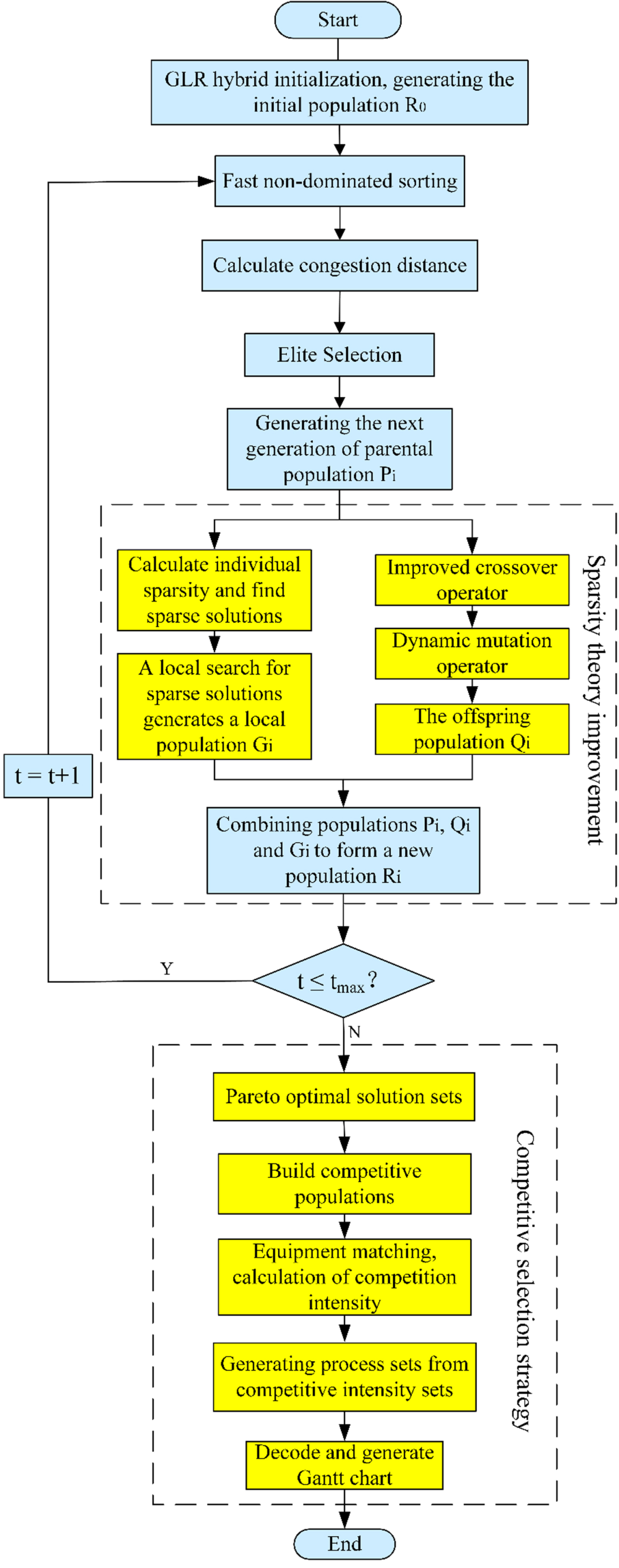
CT-NSGA-II flow chart

Generate an initial population R ₀ with size 2 N based on the GLR initialization method and set t = 0;

By fast non-dominated sorting, all individuals of the population are ranked to obtain the set of non-dominated solutions at each level F ={ F ₁, F _2,..., F _i }. For elite selection, individuals with high non-dominance rank are selected in preference, and individuals within the same non-dominance solution set are compared by calculating the crowding degree distance, and individuals with large crowding degree distance are selected in preference, whereby the next generation parent population P _i+1 is generated by merit selection with size N;

Perform crossover and mutation operations on the individuals in P _i+1 to generate the crossover offspring population Q _i+1.

calculate the sparsity for all individuals in P _i+1, find the sparse solution, and perform the local search operation on the sparse solution, thus generating the local search subgenerational population G _i+1;

Combine P _i+1, Q _i+1 and G _i+1 to obtain a new population R _i+1.

Perform the same operation as step 2 for the new population R _i+1 to generate the next generation of parent population P _i+2 with size N;

Determine whether t ⩽ t _max is valid, if not, return to Step 3 and make t = t+1; if so, execute Step 8;

Construct competing populations based on the Pareto optimal solution population set, calculate the competitive intensity

Procedure 1 Fast non-dominated sort (P)
Begin:
for eachpɛP
S_p =∅, n_p = 0
for eachqɛP
if p < q /* if p dominates q */
S_p = S_p∪ { q } /* Add q to the set of solutions governed by p */
else
n_p = n_p + 1 /* Domination count plus one */
if n_p = 0
p_rank = 1 /* The order value of p is 1 */
F₁ = F₁∪ { p } /* Add p to the first frontier */
i = 1
while F₁≠ ∅
Q =∅ /* Q is used to store the solution for the next frontier */
for each pɛF_i
for each qɛF_i
n_q = n_q - 1
if n_q = 0
q_rank = i + 1 /q belongs to the next frontier /
Q = Q∪ { q }
i = i + 1
F_i =Q
End

of each processing machine based on the process O _ij information within each competing population, and generate the set of competitive intensity of processing machines; determine the optimal solution, and decode the optimal solution to complete scheduling.

B. ALGORITHM IMPLEMENTATION PROCESS

Encoding and decoding

According to the characteristics of the multi-objective intelligent scheduling problem in the flexible workshop, the coding method adopts an extended process-based two-segment coding method, with the first segment being the process code for determining the processing order and the second segment being the machine code for determining the processing machine of the corresponding process, and the coding process is shown in Fig. 2.

Fig. 2

Process-based coding

In Fig. 2, the gene strings [1 , 1] encoded based on processes in order indicate the processes as ( O ₁₁, O ₃₁, O ₂₁, O ₂₂, O ₃₂, O ₁₂, O ₂₃, O ₁₃); the gene strings [2 , 1] encoded based on processing machines in order indicate the processing machines as ( M ₂, M ₃, M ₁, M ₃, M ₁, M ₃, M ₂, M ₁), where the positions of the genes in the gene string based on the encoding of processing machines correspond to the order of the processes in sequence, such as the position of processing machine M ₂ corresponds to the first process O ₁₁ of workpiece j ₁, the process of processing machine M ₂ corresponds to the second process O ₃₁ of workpiece j ₃, and so on.

Population initialization

In the NSGA-II algorithm, the quality of the initial population greatly affects the convergence speed and solution quality of the algorithm. The population initialization method in this paper refers to the GLR initialization method in the literature [27], i.e., a combination of global selection (GS), local selection (LS), and random selection (RS) are used to generate the initial population.

In this paper, we first execute the GLR initialization principle (the ratio of GS, LS, and RS is 0.6, 0.3 and 0.1) to generate two populations P₁, P₂ of size N, respectively, and then merge the two populations. If the number of remaining individuals in the population is greater than N, the top N individuals are selected as the initial parent population P. Otherwise, the remaining individuals are filled by the random initialization principle.

Fast non-dominated sorting

For multi-objective optimization problems, the fast-sorting method can effectively reduce the computational complexity and improve the efficiency of operations, so this paper uses the fast-sorting method to Pareto sort the individuals and grade the non-dominated solutions in the population. First, the population is set to P, the symbol n_p represents the number of dominated individuals p in the population, and the symbol S_p represents the set of dominated solutions of individual p. The description of fast non-dominated sorting is presented in Procedure 1.

Crowdedness ranking

Crowding indicates the distance between genes in the same non-dominated layer. The greater the distance between genes, the better the gene diversity. The smaller the distance between genes, the poorer the diversity. The selection of genes is based on the above idea. The gene crowding at the two endpoints of each level is defined as infinity. The crowding degree of the remaining individuals y(i) is: $P {(i)}_{distance} = \frac{(P (i + 1) f_{m} - P (i - 1) f_{m})}{(f_{m}^{\max} - f_{m}^{\min})}$ (14)

In Equation (14), P ( i ) _distance denotes the congestion distance of individual y(i), f _m denotes the value of individual y(i) as a function of target m, and $f_{m}^{\max}$ and $f_{m}^{\min}$ are the maximum and minimum values of the mth target function, respectively.

Select

The selection operation is to achieve the superiority of individuals in the population, where the individuals with higher fitness are selected with higher probability and the individuals with lower fitness are selected with lower probability. In this paper, the tournament method is used to select individuals, and two individuals are selected from the population at a time for fitness comparison, and the individual with high fitness value is put into the crossover pool. At the same time, the elite retention strategy is used to select and retain the best individuals to improve the global convergence of the algorithm.

Crossover

The crossover operation of the algorithm is performed separately for the part of workpiece sorting and the part of device selection. The workpiece sorting part uses the precedence preserving order-based crossover (POX) operation. The equipment selection part uses order-based crossover (OBX). The process is as follows:

(1) Cross-operation of work process

The work order crossover is performed using a sequence-based priority-preserving crossover operation, as shown in Fig. 3. In Fig. 3, P₁ and P₂ denote parent individuals, and C₁ and C₂ denote child individuals. First, all the workpieces are randomly divided into two subsets S₁ and S₂, and then the workpieces belonging to S₁ in P₁ are copied to C₁ and the workpieces belonging to S₂ in P₂ are copied to C₂, keeping the workpiece positions unchanged; the workpieces belonging to S₂ in P₂ are copied to C₁ and the workpieces belonging to S₁ in P₁ are copied to C₂, keeping the workpiece order unchanged.

Fig. 3

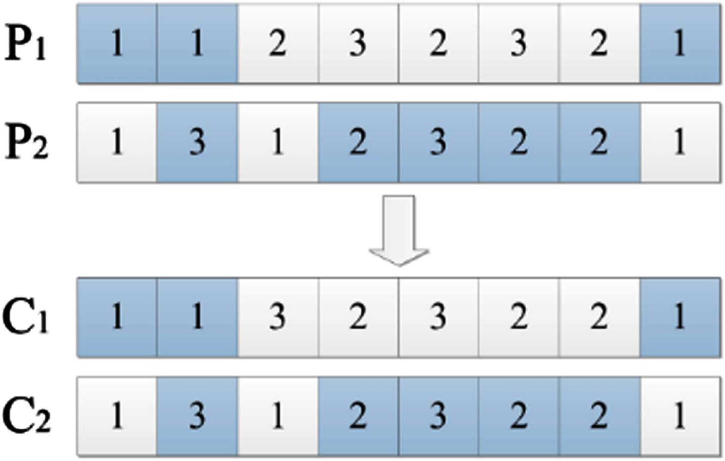
POX crossover operation

(2) Equipment cross-operation

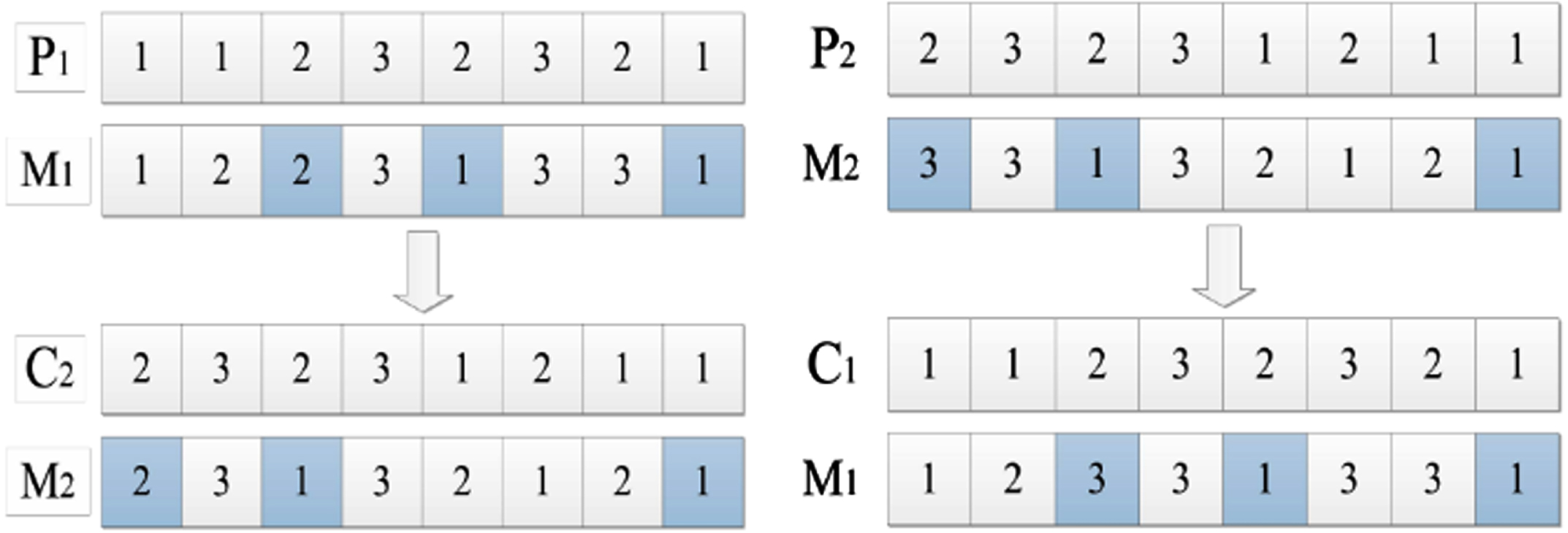
As shown in Fig. 4, equipment crossover is performed using the sequence-based crossover (OBX) operation. Here P₁, P₂, C₁, C₂ represent the same meaning as the process crossover operation and K₁, K₂, K₃, K₄ represent the subset of locations. Where K ₁ ={ 3, 5, 8 }, K ₂ ={ 1, 2, 4, 6, 7 }, K ₃ ={ 1, 3, 8 }, K ₄ ={ 2, 4, 6, 7 }. The detailed flow of equipment crossover is as follows:

Fig. 4

OBX crossover operation

Step 1: Create four subsets K₁, K₂, K₃, K₄.

Step 2: Randomly select a few position numbers from the device code and put them into K₁, and put the remaining position numbers into K₂;

Step 3: Copy the values belonging to K₂ in parent P₁ to child C₁, and copy the values belonging to K₁ in parent P₂ to child C₂, keeping the positions unchanged;

Step 4: Find the process code corresponding to K₁ in P₁ in the process code of P₂ and put its corresponding position sequence, and then put the rest of the position sequence in P₂ in K₄;

Step 5: Copy the value corresponding to K₃ in P₂ to the value corresponding to K₁ in C₁, and copy the value corresponding to K₁ in P₁ to the value corresponding to K₃ in C₂, keeping the order unchanged.

MUTATION

The mutation process of the algorithm is carried out separately for the process sequencing part and the equipment selection part.

(1) Mutation operations in the sorting part of the work order

A dynamic mutation operator is proposed for the process sorting part: there are three types of mutation operations: permutation, insertion and inverse order, and one of them is selected with equal probability for each iteration. The three mutation operations are as follows:

Swap mutation: two different positions e₁ and e₂ are randomly selected in the process code, and the elements corresponding to these two positions are exchanged.

Insert mutation: randomly select two different positions e₁ and e₂ in the process code, and insert the element corresponding to e₂ in front of e₁.

Reverse order mutation: Two different positions e₁ and e₂ are randomly selected in the process code, and the elements between these two positions are arranged in reverse order.

(2) Variant operation of the device selection section.

The mutation operation in the machine selection section performs a random replacement mutation. Two gene positions are randomly selected to replace the selected machine with any other machine from the set of its corresponding machines.

NSGA-II ALGORITHM COMBINING SPARSITY THEORY

To address the shortcomings that the crowding comparison operator in the traditional NSGA-II algorithm cannot effectively guarantee the diversity of evolving populations, and that the resulting optimal solution set is not uniformly distributed and appears premature. In this paper, we improve the diversity of the evolving population and the uniformity of the optimal solution set distribution by introducing sparsity theory [28] to find sparse solutions and performing local search on sparse solutions to obtain local search children.

(1) Calculating sparsity

The steps to obtain the sparse solution are as follows.

Step 1: In order to eliminate the differences between the objective functions of different magnitudes, the objective functions of all individuals in the population were normalized.

Let the population size be n and the number of optimization objectives be m. i is the index of individuals in the population and j is the index of the objective function. Let the objective function corresponding to individual i be ( f ₁ ( x _i) , …, f _m ( x _i)), then the jth objective function of individual i is normalized and calculated as follows: $\bar{f} (x_{i}) = \frac{f_{j} (x_{i}) - f_{jmin}}{f_{jmax} - f_{jmin}}$ (15) where f _jmax, f _jmin are the maximum and minimum values of the jth objective function value in the population. f _j ( x _i) is the function value of the jth objective function for the i-th individual.

Step 2: Calculate the Euclidean distance ρ of each individual from other individuals based on Equation (16): $ρ = \sqrt{\sum_{i = 1}^{n} {(\bar{f} (x_{i}) - \bar{f} (y_{i}))}^{2}}$ (16)

Step 3: Calculate the sparsity of each individual according to Equation (17): $SP (x_{i}) = \frac{z_{i}}{n}$ (17) where n is the number of individuals in the population. z _i is the number of individuals whose Euclidean distance between individual i and other individuals is less than k. k is the Euclidean distance judgment threshold, and its value range is 0 < k<1. If the value of k is small, the difference value of sparsity of each individual in the population is small, which is conducive to the selection of better sparse solutions. However, if the value of k is too small, a smaller clustering space is obtained, and thus a more accurate sparse solution cannot be obtained. If the value of k is large, the sparsity difference of individuals becomes larger and the solution result of the sparse solution is relatively coarser. If the value of k is too large, it is difficult to distinguish the sparsity differences of individuals, and the purpose of finding sparse solutions cannot be achieved.

3.1 Step 4: The individual with the smallest sparsity SP ( x _i) is defined as the sparse solution S*.

(2) Neighborhood Search

After the sparse solution is determined, the local search children are generated by performing a neighborhood search around the sparse solution. There are two general approaches to neighborhood search, one is to use the traditional neighborhood search structure. The other is to construct a new neighborhood structure by combining the problem characteristics and optimization objectives.

In this paper, a neighborhood search combining three neighborhood structures N₁, N₂, and N₃ is designed after considering the characteristics of the addressed problem and the encoding structure of the chromatic special. The first two neighborhood structures are related to the process code and the latter one is related to the machine code. One of N₁ ∪ N₃ and N₂ ∪ N₃ is selected with equal probability at each iteration to perform the neighborhood search operation. The specific structure is as follows.

Neighborhood structure N₁: in the process sequencing section, two processes are randomly selected and their positions in the process code are exchanged. As shown in Fig. 5(a).

Neighborhood structure N₂: select two processes at random in the process sorting code segment and insert the next process to the first position of the previous process. As shown in Fig. 5(b).

Neighborhood structure N₃: Find the machine with the highest load M_max, select a random process among all the processes on M_max, and select a random replacement machine among the backup machines for that process. As shown in Fig. 5(c).

COMPETITIVE SELECTION STRATEGY BASED ON THE STATE OF THE PROCESSING MACHINE

Fig. 5

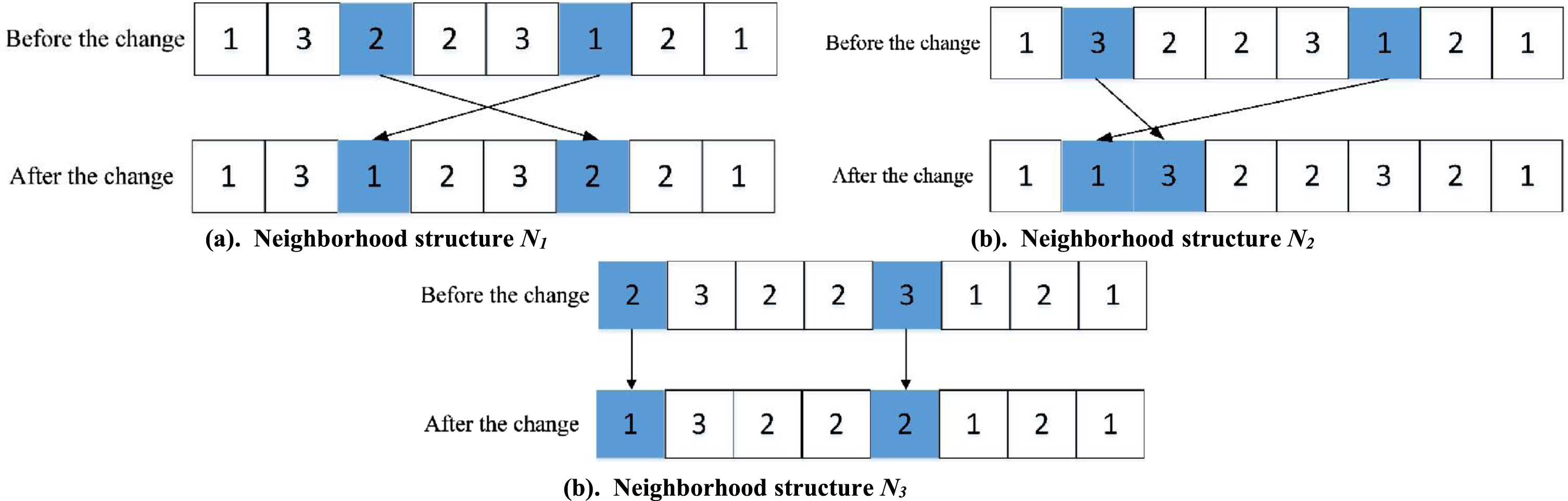
Neighborhood transform structure

The result obtained at the end of the iteration of the algorithm is a Pareto optimal solution set containing multiple individuals, and all individuals in the solution set are mutually non-dominated optimal solutions. In recent years, some scholars have also made extensive applications and explorations in the allocation, selection and scheduling of network resources by drawing on the idea of bidding mechanism [29 –31].

This paper draws on the competitive selection method of the bidding mechanism. By introducing the concept of competitive intensity, the problem of local optimum caused by information asymmetry between processing machine information and the process to be processed is reduced. Thus, the actual maximization of the set target is achieved, which is conducive to the processing machine resources to meet the objective requirements of the law of value, competition mechanism and supply-demand relationship. The sequence of processing machines and the sequence of processes to be processed can be configured more rationally. The improvement is to consider the factors such as the process energy consumption of each processing machine, the total working hours of the machine to be processed, and the idle time of the machine between the previous and subsequent processes, and use it as the basis for the process to select the optimal scheduling scheme of the appropriate processing machine.

The definition criterion R _r{ r = 1, 2, 3 } for the selection of the processing machine is described as follows:

The criterion R ₁ is the energy consumption P _ijk λ_k required for process O _ij to be processed on processing machine M _k.

The criterion R ₂ is the total time t _ijk of the process to be processed on the processing machine M _k: $t_{ijk} = \sum_{i = 1}^{n} \sum_{j = 1}^{O_{i}} P_{ijk}$ (18)

The criterion R₃ is the idle time L_ijk of the processing machine M_k under the process O_ij. $L_{ijk} = \sum_{i = 1}^{n} \sum_{j = 1}^{O_{i}} | S_{i (j + 1) k} - E_{ijk} |$ (19)

Based on the criterion R₁, criterion R₂, and criterion R₃, the competitive intensity $Y_{O_{ij}}^{k}$ of processing machine M_k for process O_ij is: $Y_{O_{ij}}^{k} = \sum_{r = 1}^{R} (\frac{R_{r}^{\max} - R_{r}^{k} (O_{ij})}{R_{r}^{\max} - R_{r}^{\min}})$ (20) where $Y_{O_{ij}}^{k}$ is the competitive intensity of processing machine M_k for process O_ij under all criteria; $R_{r}^{\max}$ and $R_{r}^{\min}$ are the maximum and minimum values selected from all available processing machines M_k as a function of process O_ij under the rth criterion, respectively; $R_{r}^{k} (O_{ij})$ is the value of machine M_k as a function of process O_ij under the rth criterion.

After determining the criteria, the steps to specify the competitive selection strategy are: first, construct the competitive population based on the Pareto optimal solution set; then, calculate the competitive strength of each processing machine based on the process O_ij information in each competitive population, and generate the competitive strength set of processing machines; second, the optimal combination of solutions in the Pareto optimal solution set is determined based on the magnitude of the competitive intensity, and the larger the value of competitive intensity, the better the solution; finally, the optimal solution in the optimal combination of solutions is determined based on the Dephi survey method, and the scheduling Gantt chart is output based on the resulting optimal solution. The Gantt chart shows the processing information of the process on the optimal processing machine and the ranking information between different processes on the same processing machine.

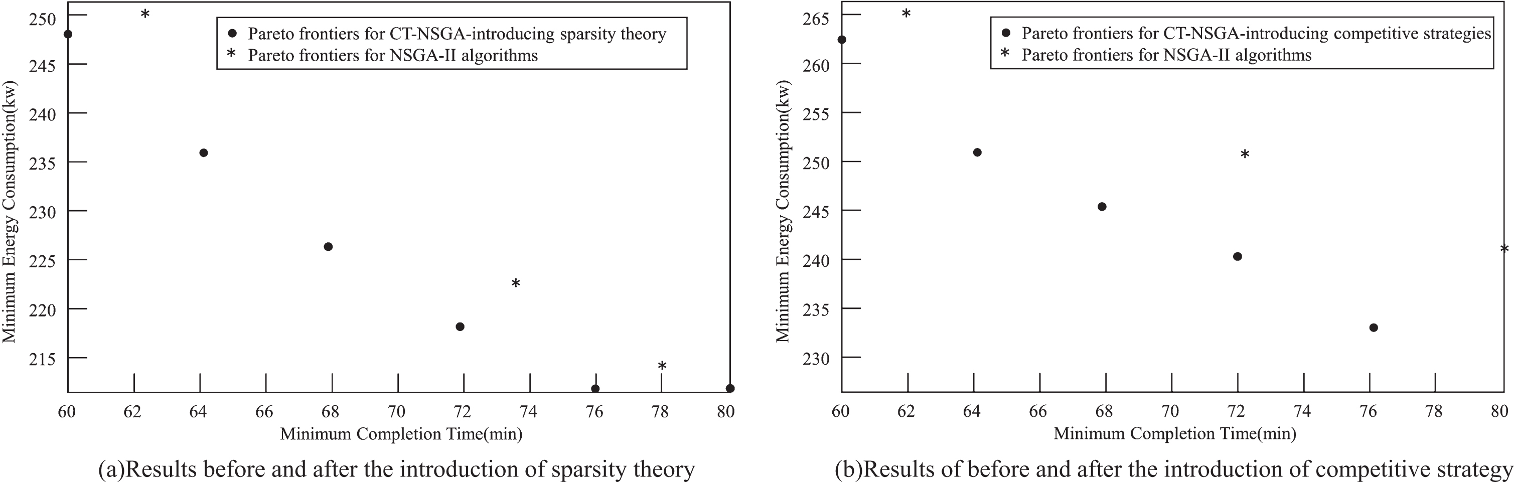
Comparing CT-NSGA-II, which introduces sparsity theory and improved operators, with the traditional NSGA-II algorithm. The processing energy rates of all equipment in the standard algorithm are randomly generated on [5, 18] and the no-load energy rates of all equipment are randomly generated on [1, 3] based on the method of literature [32]. The fixed energy consumption rate of the workshop and the transfer energy consumption of all workpieces were 30kw/h and 1.8kw/time, respectively. The data of energy consumption rate per unit time for all equipment are shown in Table 2.

Table 2

Data table of standard arithmetic energy consumption rate (kw/h)

Example	Energy consumption type	M1	M2	M3	M4	M5	M6	M7	M8	M9	M10	M11	M12	M13	M14	M15
MK01	PE	14.95	15.34	7.43	11.37	10.79	13.4
	SE	1.24	2	2.92	1.68	2.17	1.45
MK02	PE	14.77	8.32	11.58	14.09	16.58	17.47
	SE	2.09	1.28	1.3	1.52	2.68	1.51
MK03	PE	15.59	8.17	17.08	9.55	7.56	8.26	13.01	11.15
	SE	1.7	2.66	2.17	2.1	2.83	1.57	2.51	2.51
MK04	PE	9.95	12.38	5.99	5.7	11.9	15.13	17.14	6.69
	SE	2.14	1.94	1.02	1.67	1.32	2.59	1.62	2.06
MK05	PE	7.15	12.83	8.42	13.5
	SE	2.38	2.5	1.9	1.17
MK06	PE	5.06	15.07	15.62	16.29	6.1	10.2	8.38	15.4	10.61	16.84
	SE	1.46	2.83	1.3	2.65	2.08	2.99	1.16	1.89	1.21	2.92
MK07	PE	7.36	8.43	6.89	6.77	16.3
	SE	2.16	2.1	1.29	2.71	2.24
MK08	PE	9.56	11.67	10.22	5.99	8.12	6.6	7.39	8.12	10.42	5.65
	SE	2.81	2.89	1.98	1.98	1.68	2.8	1.74	1.22	2.56	1.78
MK09	PE	8.14	10.25	6.25	6.72	17.25	17.43	12.48	5.78	8.05	9.59
	SE	2.64	1.03	1.09	1.34	2.3	2.46	2.3	1.9	2.09	1.59
MK10	PE	14.68	7.46	13.93	7.39	9.8	15.13	14.14	6.05	17.18	15.46	11.33	10.66	10.17	10.88	8.98
	SE	2.02	2.64	2.59	2.29	1.76	2.62	2.07	1.7	2.88	2.75	2.1	2.25	2.15	1.15	1.7

Using the machine processing time as well as the processing cost information, minimizing the completion time and the production energy consumption as the optimization objectives for the experiments, the standard algorithms are solved separately. Taking MK04 as an example, the experimental results are shown in Fig. 6. It can be seen that the solution quality and distribution of the CT-NSGA-II algorithm are better than the original algorithm.

Fig. 6

Comparison of experimental results between the CT-NSGA-II and the NSGA-II.

4 Experimental simulation and analysis

In this section, we first set the tuning parameters for the operation of the algorithms. Next, the standard algorithms are solved and verified using each of the three algorithms. Finally, the CT-NSGA-II algorithm is applied to the engineering cases to verify its effectiveness.

A. ALGORITHM PARAMETER TUNING

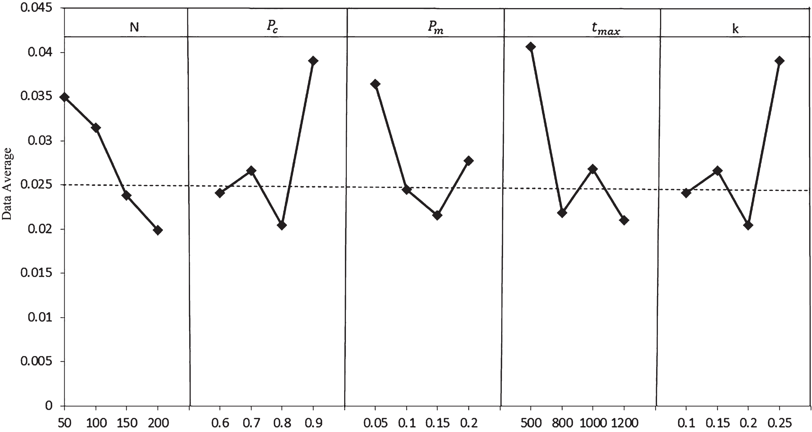
The algorithm parameters of CT-NSGA-II are set to include: population size N, crossover probability P_c, mutation probability P_m, maximum evolutionary generation t_max, and individual sparsity discriminant threshold k in sparsity theory.

The method of parameter tuning is to analyze the effect of different settings of five parameters on the optimization results by using the Taguchi method with MK01 as the test example, so as to find out the better parameter setting scheme.

Four reasonable level values for the five parameters are given in Table 3, and the corresponding 16 parameter combination schemes are given in Table 4. For each parameter combination setting method, the CT-NSGA-II algorithm was run 10 times independently.

Table 3
The values of the five parameters

Parameters Level value

1 2 3 4

N 50 100 150 200

P_c 0.6 0.7 0.8 0.9

P_m 0.05 0.1 0.15 0.2

t_max 500 800 1000 1200

k 0.1 0.15 0.2 0.25

Parameters	Level value
N	50	100	150	200
P_c	0.6	0.7	0.8	0.9
P_m	0.05	0.1	0.15	0.2
t_max	500	800	1000	1200
k	0.1	0.15	0.2	0.25

Table 4

The way the five parameters are combined and their response values

Experimental	Parameters					IGD
combinations	N	P_c	P_m	t_max	k
1	50	0.6	0.1	500	0.1	0.0408
2	50	0.7	0.15	800	0.15	0.0297
3	50	0.8	0.2	1000	0.2	0.0351
4	50	0.9	0.05	1200	0.25	0.0343
5	100	0.6	0.15	800	0.1	0.0226
6	100	0.7	0.2	1000	0.15	0.0429
7	100	0.8	0.1	1200	0.2	0.0116
8	100	0.9	0.05	500	0.25	0.0489
9	150	0.6	0.2	1000	0.1	0.0146
10	150	0.7	0.15	1200	0.15	0.0196
11	150	0.8	0.1	800	0.2	0.0169
12	150	0.9	0.05	500	0.25	0.0443
13	200	0.6	0.2	1200	0.1	0.0184
14	200	0.7	0.15	1000	0.15	0.0144
15	200	0.8	0.05	800	0.2	0.0181
16	200	0.9	0.1	500	0.25	0.0286

Since it is a multi-objective optimization problem, the average value of the inverse generation distance (IGD) is chosen as the response value [33]. The resulting average response values of each parameter are shown in Table 5. From Table 5, it can be seen that the different values of the five parameters lead to a large difference in the variation of the corresponding average response values. The maximum number of iterations was 0.0196 at the four levels, followed by a discriminant threshold of 0.0183 for individual sparsity, 0.0183 for crossover probability, 0.0150 for population size, and 0.0147 for variance probability.

Table 5

Average response values for the five parameters

Level value	N	P_c	P_m	t_max	k
1	0.0349	0.0241	0.0364	0.0406	0.0241
2	0.0315	0.0266	0.0244	0.0217	0.0266
3	0.0238	0.0204	0.0215	0.0266	0.0204
4	0.0198	0.0391	0.0275	0.0209	0.0390
Differences	0.0150	0.0183	0.0147	0.0196	0.0183
Sort	4	3	5	1	2

The trend graphs of the response values of the five parameters are shown in Fig. 7. Analysis of Fig. 7 shows that t_max has the greatest effect on the optimization results, and the other four parameters have a smaller effect. Therefore, the CT-NSGA-II algorithm is optimized best with the parameter values N = 200, P_c = 0.8, P_m = 0.15, t_max = 1200, and k = 0.2. Therefore, this setting scheme is uniformly adopted for the parameters of the CT-NSGA-II algorithm and NSGA-II algorithm in the experiments of this chapter.

Fig. 7

Graph of response trend of parameters

B. SIMULATION ANALYSIS OF STANDARD ALGORITHMS

In this section, CT-NSGA-II, the conventional NSGA-II algorithm [18], and the MOEA/D algorithm [34], which aims to minimize the total energy consumption and cost, are used to solve the standard examples, respectively. We choose 10 BRdata FJSP benchmarks (Mk01-Mk10) to test the performance of the algorithm. The solution method used in this paper was implemented using C# language, and the computational program was run on MATLAB 2016b platform and visual studio 2013 with computer configuration of Intel(R) Core (TM) i7-7700HQ CPU @2.80 GHz, 8.00 GB RAM.

To effectively apply the above algorithm for the solution, Based on the literature [35], the delivery date data for all workpieces are generated according to Equation (21). $d_{j} = r_{j} + t_{j} \times \sum_{l = 1}^{s_{j}} p_{l, j}$ (21)

In Equation (21), d_j represents the delivery time of the jth workpiece, r_j represents the placement time of the jth workpiece, t_j represents the looseness of the jth workpiece, s_j represents the total number of processes of the workpiece, and p_l,j represents the processing time of the workpiece O_l,j. The values of t_j can be taken as 2,1.5,1, which represent time lax, moderate, and tight, respectively. Based on the literature [36], the different time laxity (tight, moderate, loose) are set to 34%,33%,33% in each case.

The parameters of the CT-NSGA-II algorithm and NSGA-II algorithm were set according to the parameters after tuning in the previous section. The corresponding weights of f₁, f₂, and f₃ are obtained by Delphi survey method as 0.3,0.3,0.4.

The parameter settings of the MOEA/D algorithm are referred to the literature [34]. Its aggregation function uses Chebyshev aggregation method. The population size is set to 62, the probability of mutation is set to 1.0, the number of splits is set to 10, the size of the weight vector neighborhood is set to 20, the maximum number of replaceable solutions per child is set to 1, and the maximum number of iterations is set to 1200. the above three cases are run 10 times to take the average value, and the simulation results are shown in Table 6 below. In Table 6, “best” represents the best value and “avg” represents the average value.

Table 6

Simulation results of standard algorithm

Algorithm size	Algorithm	Optimization Goals
		f₁/min	f₂/min	f₃/kw
		avg	avg	avg
MK01	NSGA-II	43.3	0.7	142.19
	CT-NSGA-II	42.0	1.7	139.50
	MOEA/D	42.0	3.7	140.46
MK02	NSGA-II	33.3	1.3	118.53
	CT-NSGA-II	34.0	0.0	112.06
	MOEA/D	34.3	0.0	115.09
MK03	NSGA-II	204.3	41.3	493.39
	CT-NSGA-II	208.3	15.0	485.96
	MOEA/D	208.0	28.0	494.60
MK04	NSGA-II	69.7	37.7	242.94
	CT-NSGA-II	68.0	21.7	244.10
	MOEA/D	68.7	28.0	245.40
MK05	NSGA-II	177.3	757.7	387.29
	CT-NSGA-II	185.3	681.3	399.13
	MOEA/D	186.0	810.3	401.16
MK06	NSGA-II	78.0	0.0	357.07
	CT-NSGA-II	74.7	0.0	358.44
	MOEA/D	84.0	0.0	363.77
MK07	NSGA-II	146.7	140.3	354.39
	CT-NSGA-II	144.8	97.3	355.56
	MOEA/D	155.6	288.3	368.16
MK08	NSGA-II	522.9	2810.7	1097.15
	CT-NSGA-II	524.0	2680.0	1095.89
	MOEA/D	527.3	2666.3	1114.80
MK09	NSGA-II	315.7	457.0	999.25
	CT-NSGA-II	314.3	408.3	998.48
	MOEA/D	349.7	739.7	1026.63
MK10	NSGA-II	374.7	1484.0	1247.33
	CT-NSGA-II	372.3	1524.7	1245.00
	MOEA/D	256.0	243.1	1063.35

Analyzing Table 6, we can see that for the index of maximum completion time, the CT-NSGA-II algorithm obtains the optimal average value for 5 cases of MK01, MK04, MK06, MK07, MK09. The NSGA-II algorithm obtains the optimal average value for 4 cases of MK02, MK03, MK05, and MK08. The MOEA/D algorithm obtained the optimal average of 2 cases, MK10, MK02, MK03, MK05 and MK08. The CT-NSGA-II algorithm obtains the optimal average value for 7 cases of MK02-MK07, MK09, and 2 cases of MK01, MK06, and the MOEA/D algorithm obtains the optimal average value for 4 cases of MK02, MK06, MK08, and MK10. For the total energy consumption objective: CT-NSGA-II algorithm obtained the optimal average value for 5 cases of MK01-MK03, MK08, MK09. NSGA-II algorithm obtained the optimal average value for 4 cases of MK04-MK07. MOEA/D algorithm obtained the optimal average value for 1 case of MK10.

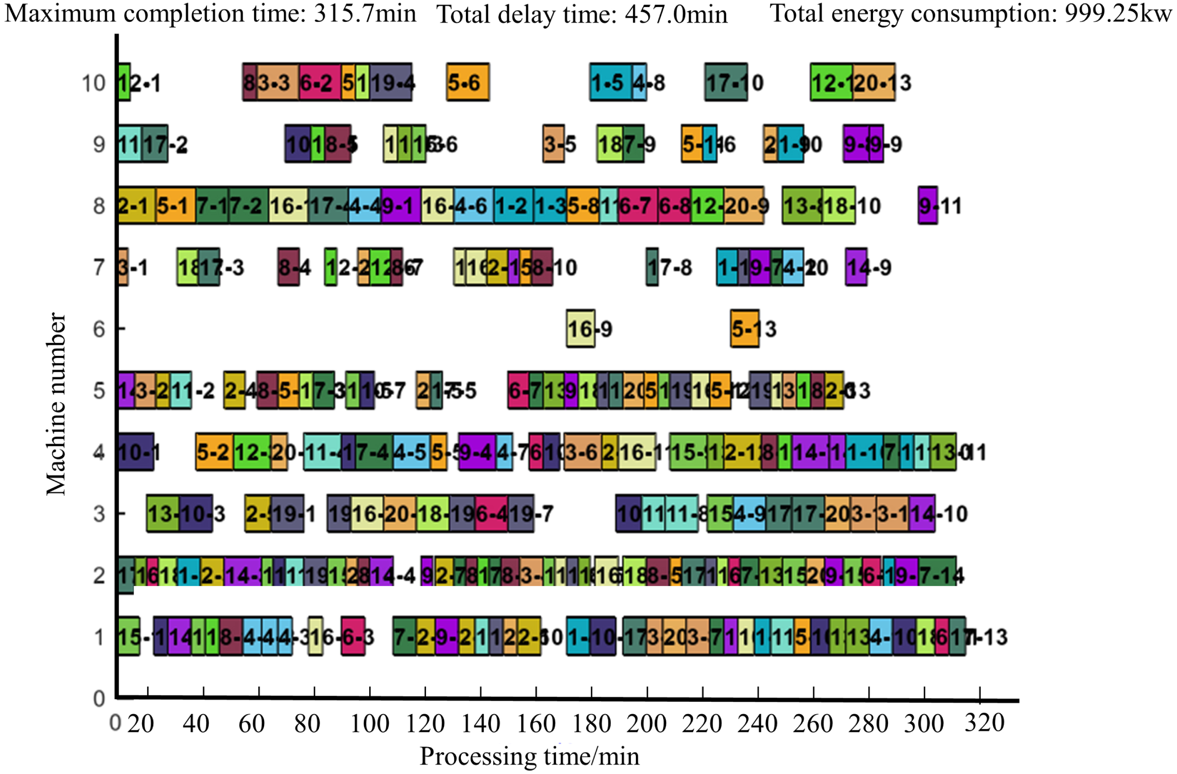
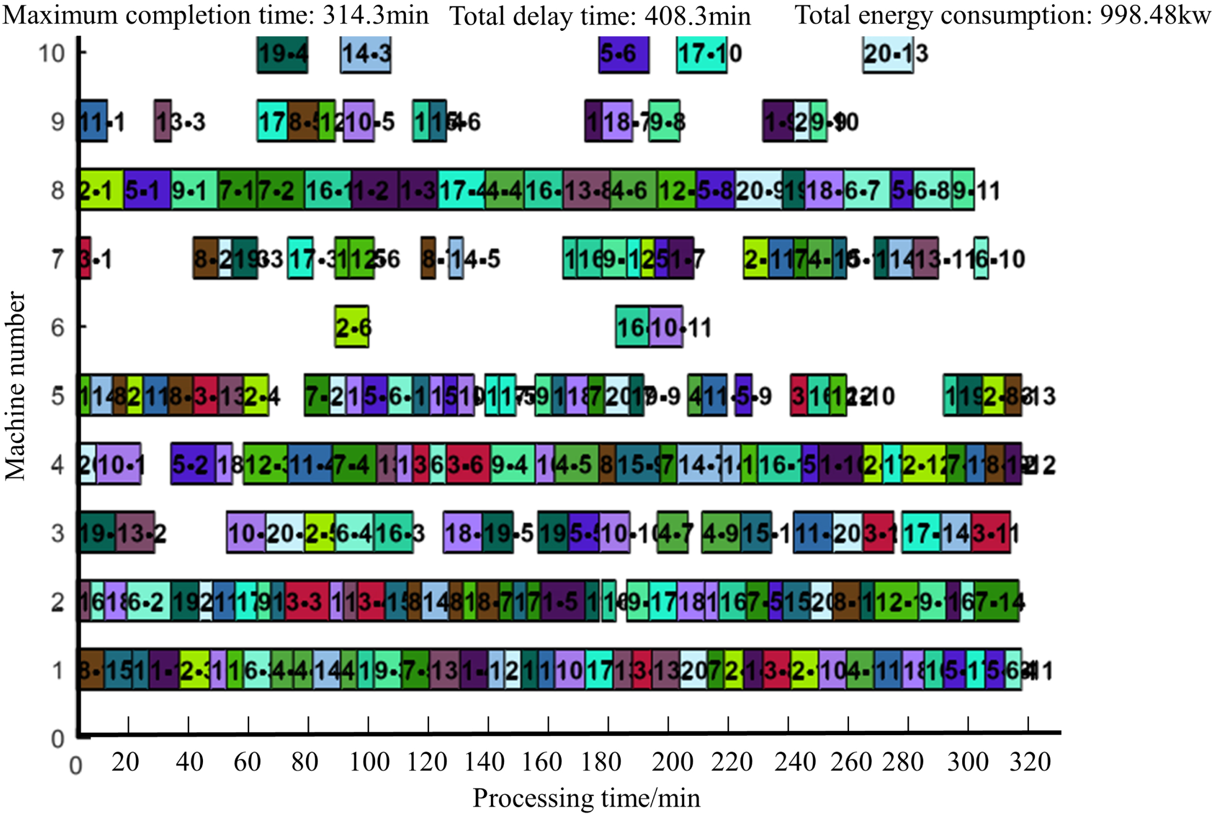
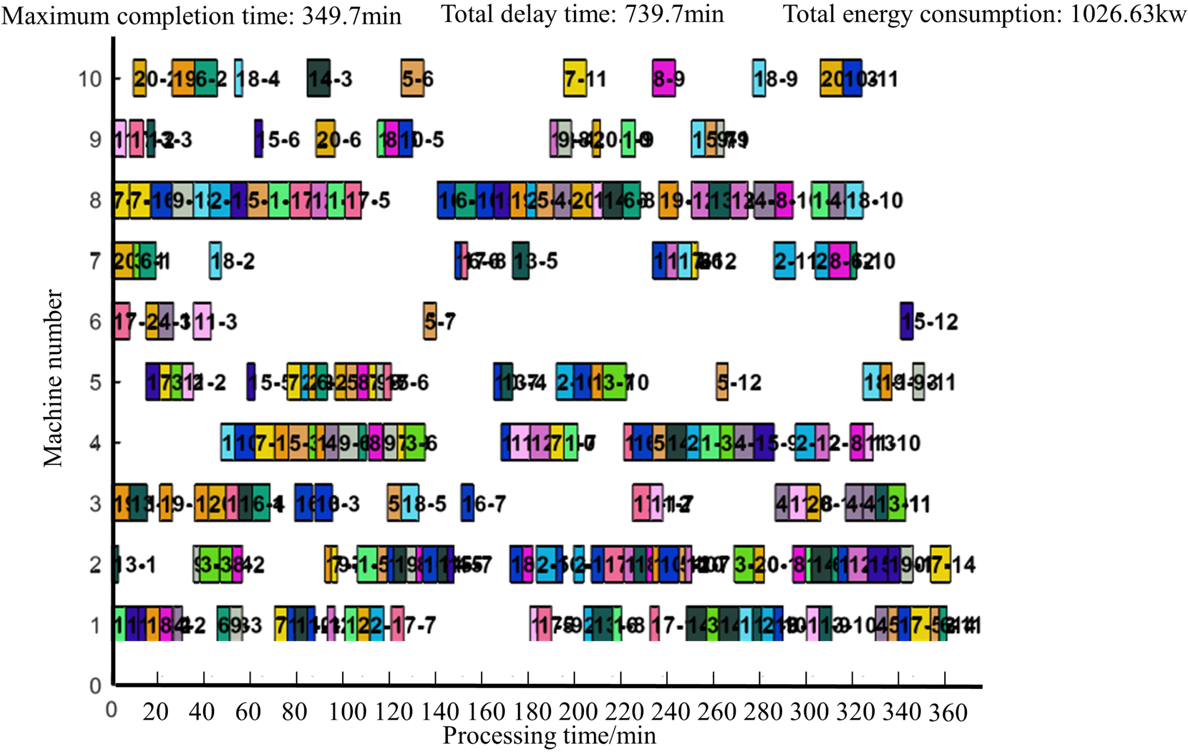
Taking MK04 as an example, the corresponding Gantt charts after solving the three algorithms are shown in Figs. 8, 9, and 10. From the scheduling results of the Gantt charts, it can be seen that the scheduling solution generated by CT-NSGA-II can effectively shorten the completion time and delay time and reduce the processing energy consumption. Therefore, the CT-NSGA-II algorithm outperforms the NSGA-II algorithm and the MOEA/D algorithm in solving the flexible job shop scheduling under the standard cases in terms of solution accuracy.

Fig. 8

NSGA-II Solving Gantt Chart for MK04 Scheduling Results

Fig. 9

CT-NSGA-II Solving Gantt Chart for MK04 Scheduling Results

Fig. 10

MOEA/D solving Gantt chart for MK04 scheduling results

CT-NSGA-II does not get the optimal solution every time in large-scale instances, but the scheduling of the CT-NSGA-II algorithm is able to achieve more optimal values in terms of the combined effect. Taking MK09 as an example, CT-NSGA-II achieves the optimal solution in all three optimization objectives: maximum completion time, total extension time, and total energy consumption. The Gantt charts corresponding to the three algorithms after solving are shown in Figs. 11–13.

Fig. 11

NSGA-II Solving Gantt Chart for MK09 Scheduling Results

Fig. 12

CT-NSGA-II solving Gantt chart forMK09 scheduling results

Fig. 13

MOEA/D solving Gantt chart for MK09 scheduling results

C. ALGORITHM PERFORMANCE ANALYSIS

In order to verify the effectiveness of the algorithm proposed in this paper more comprehensively, this section uses the super volume and the inverse generation distance, which are common evaluation metrics for the performance of multi-objective optimization algorithms, as evaluation metrics. The validity of the proposed neighborhood structure is first verified under the same algorithm, and then the standard cases are solved using different algorithms to verify the superiority of the algorithm in this paper.

1) Performance evaluation index

The inverse generation distance (IGD) [33] is used as a comprehensive metric to evaluate both the convergence and the distribution performance of the solution set. To calculate the IGD, a set of reference points uniformly distributed over the real Pareto fronts is required. The smaller the IGD value, the better the fit of the solution set to the Pareto frontier. The ideal Pareto front surface is generated as an approximate combination of the optimal set of solutions obtained by the algorithm over many solutions. The real Pareto frontier in this case is the approximate frontier obtained by aggregating the solution sets obtained from all the tested algorithms run 10 times each. The IGD calculation formula is as follows. $IGD = \frac{\sum_{i = 1}^{| PF |} distance (p, cr)}{| PF |}$ (22)

In Equation (22), PF is the true Pareto front of the multi-objective optimization problem; |PF| is the scale of the true Pareto front of the problem; cr is the point on the approximate Pareto front created by the multi-objective optimization algorithm; p is the point on the true Pareto front; the function distance() is used to calculate PF and the shortest distance from a point p on PF to the approximate Pareto front distance(p,cr).

Convergence and diversity are also generally considered when evaluating the performance of an algorithm. the HV measure (supervolume measure) [32], a classical one-dimensional measure in multi-objective optimization, can accurately visualize the diversity and convergence of the Pareto solution set. The larger the HV value, the better the overall performance of the algorithm. In calculating the HV value, a reference point needs to be given in advance. In this paper, the reference point is set to the true optimal boundary, which is 1.1 times the maximum value of each target dimension. The HV measure is calculated as in equation (23), where vol(a) denotes the volume of the hypercube enclosed by some non-dominated solution a of algorithm A and the reference point. $HV (A) = \underset{a \in A}{\cup} vol (a)$ (23)

2) Model Correctness Verification

In order to verify the correctness of the constructed model, this section solves the model with the single objectives of completion time, delay time, and energy consumption, respectively, by referring to the multi-objective algorithm in the literature [38] compared with CPLEX. The deviation amounts of the three objectives obtained by solving CPLEX with the CT-NSGA-II algorithm are compared, and the CPU running times of the two methods are recorded. Considering the limitation of the scale of the CPLEX solving problem, the small-scale cases of MK01-MK05 are selected for solving based on the parameter setting in the previous section. In this paper, in order to speed up the solution of CPLEX and reduce the solution time, the gap is set not to be 0, multiple feasible solutions are pursued, and the optimal solution is selected among the output multiple feasible solutions. Although Gap is not 0, the solver output is close to the optimal solution and can be used to verify the correctness of the model. The comparison results are shown in Table 7.

Table 7

Comparison results of CT-NSGA-II and CPLEX

Cases	Completion time/min		Completion time deviation/%	Delay time/min		Delay time deviation/%	Energy consumption/kw		Energy consumption deviation/%	CPU runtime/s
	CPLEX	CT-NSGA-II		CPLEX	CT-NSGA-II		CPLEX	CT-NSGA-II		CPLEX	CT-NSGA-II
MK01	42.2	42.0	0.4	1.8	1.7	5.8	141.2	139.8	1.0	3.6	3.1
MK02	35.6	34.7	2.5	0	0	0	113.1	112.6	0.4	4.8	4.4
MK03	212.1	208.2	1.9	16.1	15.3	5.2	490.6	485.9	1.0	5.8	4.7
MK04	69.1	68.0	1.6	22.5	21.7	3.6	246.9	244.1	1.1	8.4	5.9
MK05	189.2	185.3	2.1	693.4	681.3	1.7	403.8	399.2	1.2	20.6	9.5

As can be seen from Table 7, the solutions obtained by the CT-NSGA-II algorithm solution are very close to the CPLEX solution results under the small-scale arithmetic example, which verifies the correctness of the model in this paper. In the five sets of cases, the maximum deviation of completion time between CT-NSGA-II and CPLEX is 2.5%, the maximum deviation of delay time is 5.2%, and the maximum deviation of energy consumption is 1.2%, which are all within the acceptable range. In addition, the CT-NSGA-II algorithm can save more solution time than CPLEX when the case size gradually increases.

3) Neighborhood structure validation

In order to explore the effectiveness of the proposed neighborhood search strategy, this section compares CT-NSGA-II with itself after removing the neighborhood search, and the algorithm after removing the neighborhood search is called CNINNS (CT-NSGA-II with no neighborhood search) here. The parameters of both algorithms were set as in the previous section. To overcome the random error, both algorithms were run 10 times independently for each test problem and the statistical results were taken for comparison. The results of CT-NSGA-II and CNINNS runs on the 10 test problems regarding IGD and HV are given in Table 8.

Table 8

Solution results of CT-NSGA-II and CNINNS arithmetic cases

Example	IGD		HV
	CT-NSGA-II	CNINNS	CT-NSGA-II	CNINNS
MK01	0.0132	0.0236	1.0284	1.0278
MK02	0.0233	0.0493	1.2049	1.2031
MK03	0.0405	0.0407	1.0368	1.0351
MK04	0.0337	0.0393	1.0158	0.9744
MK05	0.0482	0.0554	0.5636	0.5624
MK06	0.0595	0.0598	1.0250	1.0252
MK07	0.0623	0.0644	0.7998	0.7899
MK08	0.0730	0.0745	0.7914	0.7881
MK09	0.0720	0.0775	1.0009	0.9952
MK10	0.1141	0.1199	0.8861	0.8789

As can be seen in Table 8, for the IGD and HV measurement values, the difference between CT-NSGA-II and CNINNS is small on a few instances (MK03/MK06). However, CT-NSGA-II significantly outperforms CNINNS on the remaining test instances. As a whole, CNINNS did not outperform CT-NSGA-II in any of the measured cases. Therefore, it can be concluded that the proposed novel neighborhood structure can improve the convergence of the algorithm to some extent.

4) Analysis of algorithm operation results

The solution results of CT-NSGA-II algorithm, NSGA-II algorithm and MOEA/D algorithm for the above ten standard cases are compared and analyzed. Here the parameters of the three algorithms are set as in the previous section. In order to overcome the random error, all three comparison algorithms are run independently for 10 times and the average results are taken. The results are shown in Table 9, and the key data have been bolded.

Table 9

Statistical results of IGD

Example	IGD			HV
	CT-NSGA-II	NSGA-II	MOEA/D	CT-NSGA-II	NSGA-II	MOEA/D
MK01	0.0132	0.0335	0.0201	1.0284	1.0393	1.0644
MK02	0.0233	0.0731	0.0310	1.2049	1.1065	1.4224
MK03	0.0405	0.0417	0.0358	1.0368	0.9749	0.6844
MK04	0.0337	0.0428	0.0496	1.0158	0.9619	0.9265
MK05	0.0482	0.0717	0.1133	0.5636	0.5607	0.4550
MK06	0.0595	0.0427	0.0464	1.0250	1.0045	0.9641
MK07	0.0623	0.0731	0.0907	0.7998	0.7623	0.6569
MK08	0.0730	0.0765	0.0783	0.7914	0.7851	0.7636
MK09	0.0735	0.0720	0.0854	0.8106	0.8162	0.7023
MK10	0.1141	0.1320	0.0829	0.8861	0.8770	0.6224

Compared with the other two algorithms, the CT-NSGA-II algorithm achieves optimal IGD values for all seven cases except MK03, MK06 and MK10. It also achieves the second best IGD value for solving MK03 and MK10, the best HV value for solving all 8 cases from MK03 to MK10, and the second best HV value for solving MK02. NSGA-II achieves optimal IGD values for solving MK06 cases, suboptimal IGD values for solving MK04-MK05, MK07-MK09, and suboptimal HV values for solving MK01, MK03-MK10 cases. MOEA/D achieves optimal IGD values for solving a total of 2 cases, MK03 and MK10, and optimal HV values for solving the MK01-MK02 cases.

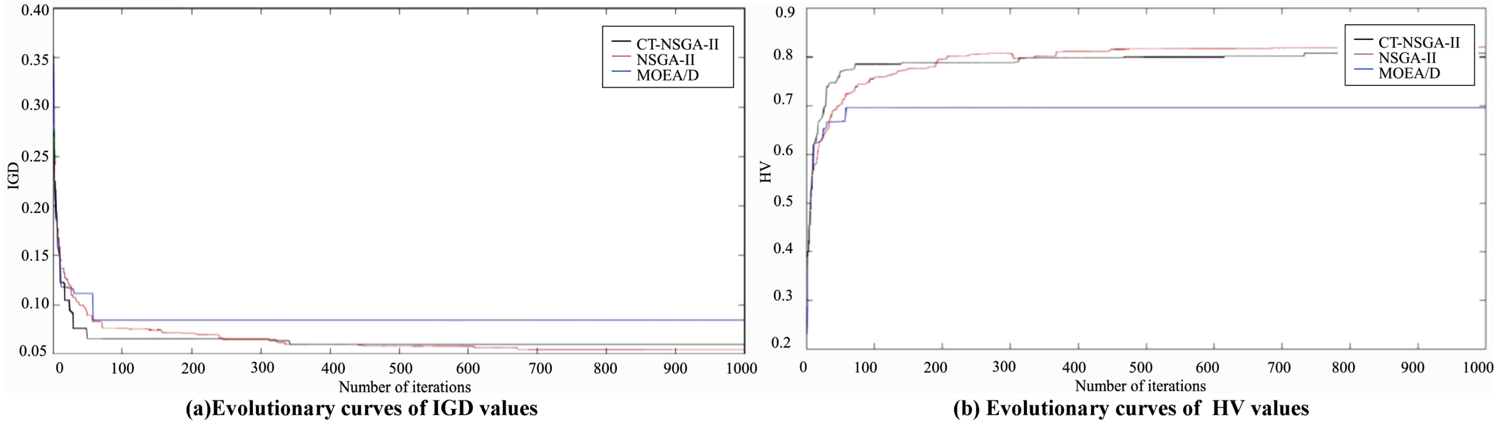
Figures 14–17 show the evolutionary convergence plots of HV and IGD values obtained when solving examples MK04, MK05, and MK06 for CT-NSGA-II, NSGA-II, and MOEA/D algorithms, respectively. Analysis of the curves shows that: during the evolutionary process, the IGD values of all three algorithms are decreasing and the HV values are increasing. Moreover, the IGD and HV values decreased and increased significantly between 0 and 100 iterations, and the decrease and increase of IGD and HV values slowed down after 100 iterations. Finally, all three algorithms converge after 100 iterations. However, the IGD evolution curve of CT-NSGA-II is always below the other two algorithms between 100 and 1000 iterations, and its HV evolution curve is always above the other two algorithms between 100 and 1000 iterations. The above analysis shows that the CT-NSGA-II algorithm can achieve better HV and IGD values than the MOEA/D algorithm and NSGA-II algorithm, and its comprehensive performance of multi-objective optimization is better.

Fig. 14

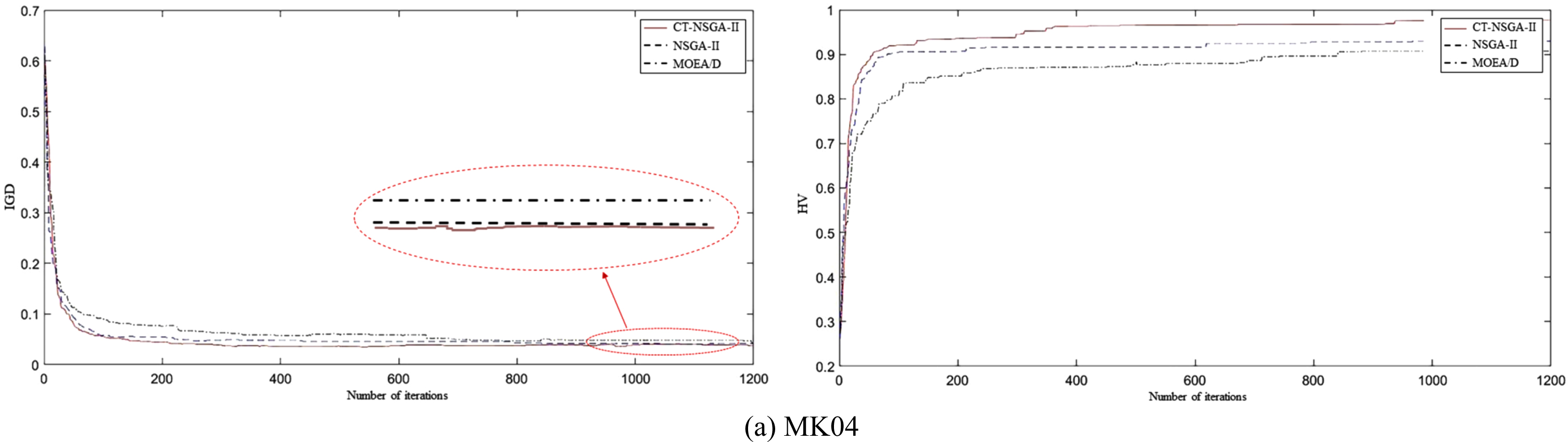
Evolutionary curves of IGD values and HV values obtained from three algorithms solving MK04

Fig. 15

Evolutionary curves of IGD values and HV values obtained from three algorithms solving MK05

Fig. 16

Evolutionary curves of IGD values and HV values obtained from three algorithms solving MK06

Fig. 17

Evolutionary curves of HV values obtained from three algorithms solving different cases

D. ENGINEERING CASE ANALYSIS

In order to further verify the effectiveness of the model and algorithm, the actual production data of the manufacturing production plant of Company A is used as a case, and two algorithms, NSGA-II and CT-NSGA-II, are used to simulate and solve it. The processing information is shown in Table 10 and Table 11, which shows that the case belongs to the 10×6 FJSP problem. The simulation environment and the parameter settings of the two algorithms are the same as in the previous section.

Table 10

10*6 FJSP problem

Workpiece	Work serial	Equipment	Processing	Delivery
number	number	number	time /min	Period /min
Workpiece 1	1	1,3,5	15,21,25	120
	2	2,6	14,17
	3	1,3,4,5	11,10,21,14
	4	2,5,6	8,12,11
Workpiece 2	1	2,3,5	22,23,18	85
	2	3,4	20,22
	3	1,5,6	12,15,14
Workpiece 3	1	3,4,5	18,17,13
	2	2, 5,6	8,11,14	140
	3	1,2,3	18,17,18
	4	5,6	18,19
	5	1,2,6	19,17,16
Workpiece 4	1	4,5,6	20,22,23	95
	2	1,2,4	16,17,16
Workpiece 5	1	3,4	20,25	105
	2	1,2,4,6	24,18,25,20
	3	1,2,5,6	20,15,22,19
	4	1,4	10,12
Workpiece 6	1	1,3,4,5	23,21,17,18	160
	2	2,3,4,6	8,12,17,11
	3	4,6	12,15
	4	2,3,5	15,21,25
	5	2,5	19,12
Workpiece 7	1	5,6	12,19	115
	2	1,2,3,4	12,15,14,9
	3	2,5,6	8,9,11
Workpiece 8	1	1,4,5,6	11,9,14,13	135
	2	2,6	10,12
	3	1,3,5	20,17,14
	4	1,3	19,17
Workpiece 9	1	1,2,3	11,10,14	150
	2	2,4,5	8,12,19
	3	2,4,6	15,21,25
	4	1,5	18,19
	5	2,5,6	12,15,14
	6	4,5	7,10
Workpiece 10	1	2,4,5	18,17,20	70
	2	1,2,3,4	8,11,9,16
	3	3,4	14,17

Table 11

10*6 FJSP energy consumption data

Equipment number	PE/(kw/h)	SE/(kw/h)
1	20	3.45
2	25	2.82
3	6	0.84
4	12	1.58
5	10	1.41
6	5.5	0.55

In the energy consumption data in Table 11 the fixed energy consumption is 35kw/h and the transfer energy consumption is 2kw per time.

The simulation solution of the above example can be obtained as shown in Figs. 18–20, and the analysis shows that:

Fig. 18

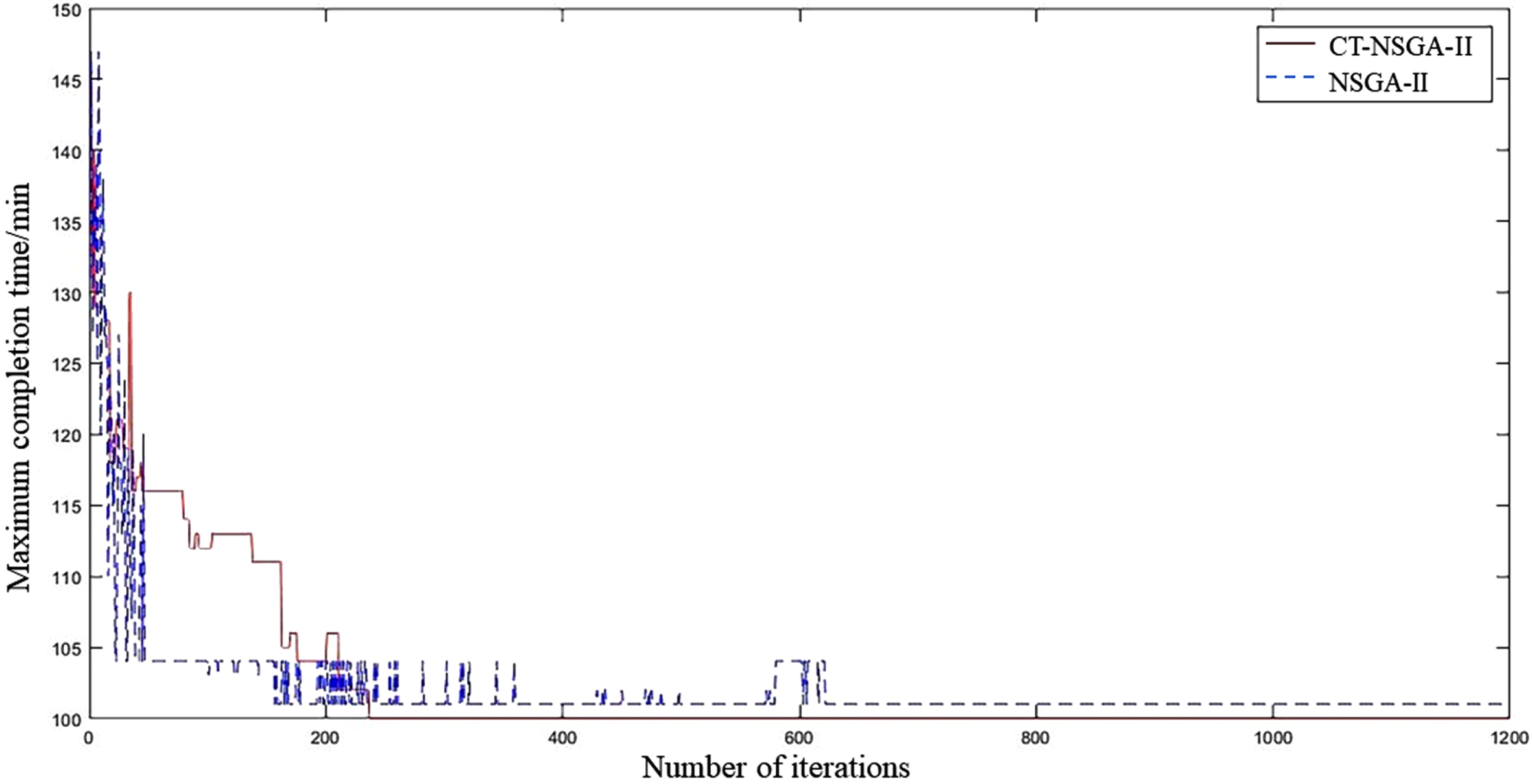
Maximum completion time convergence curves obtained by two algorithms for solving the 10*6 FJSP problem

Fig. 19

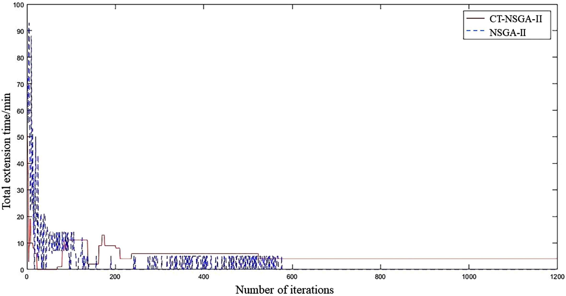
Convergence curves of the total extension time obtained by two algorithms for solving the 10*6 FJSP problem

Fig. 20

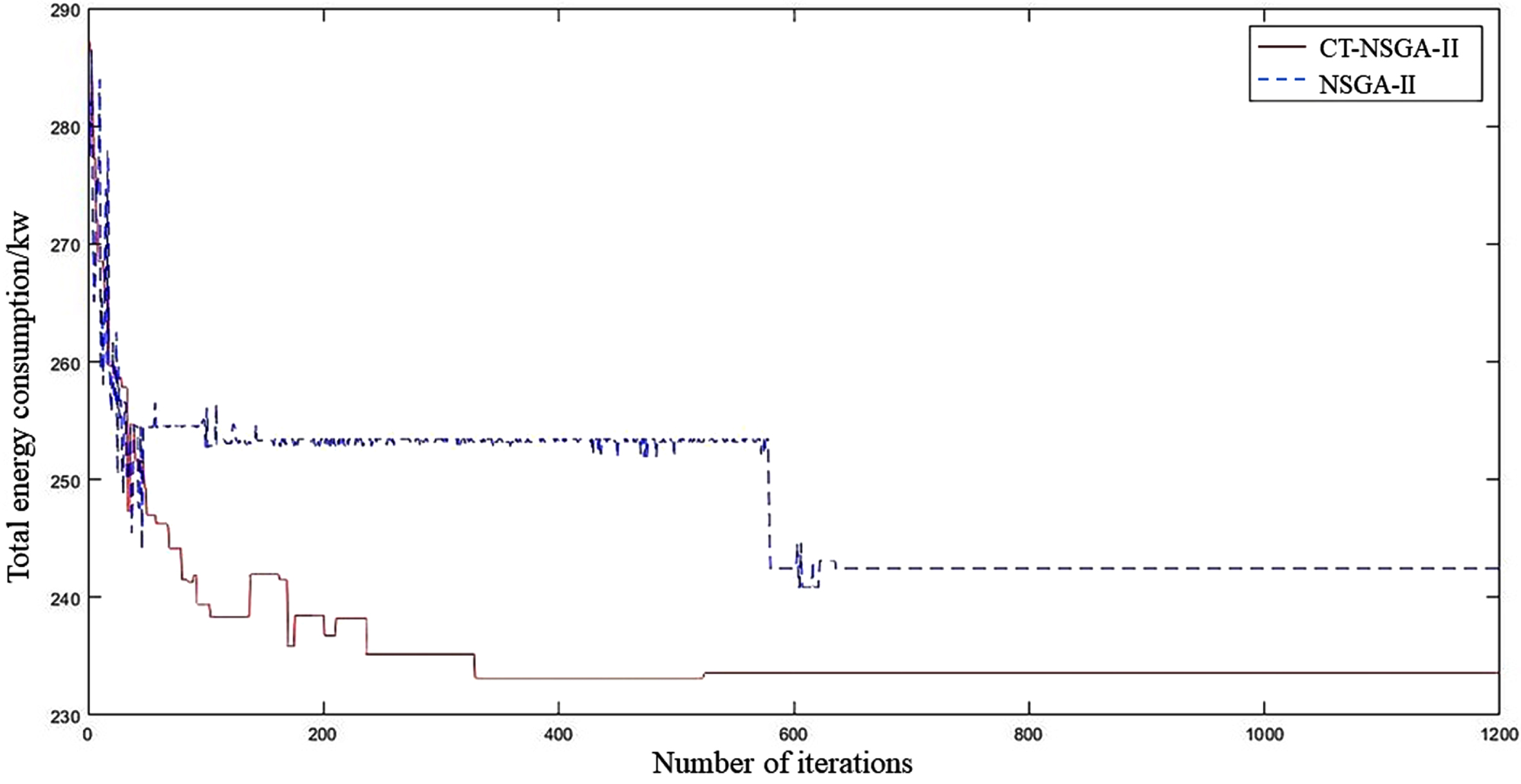
Convergence curves of the total energy consumption obtained by two algorithms for solving the 10*6 FJSP problem

1) The CT-NSGA-II algorithm outperforms the NSGA-II algorithm in both total energy consumption and maximum completion time, but the NSGA-II algorithm slightly outperforms the CT-NSGA-II algorithm in total extension time. The main reason is that the energy consumption of the equipment generally decreases as the total load of the equipment increases. As a result, the increased equipment load, reduced energy consumption and completion time may result in longer delivery dates for some orders.

2) NSGA-II algorithm curve is more volatile, CT-NSGA-II algorithm curve is smoother. The reason is that when the NSGA-II algorithm solves the low-dimensional MOP problem, the number of solutions in the Pareto solution set is largely due to the poor population diversity, which leads to a large difference in the optimal compromise solution selected each time and makes the optimal solution uncertain.

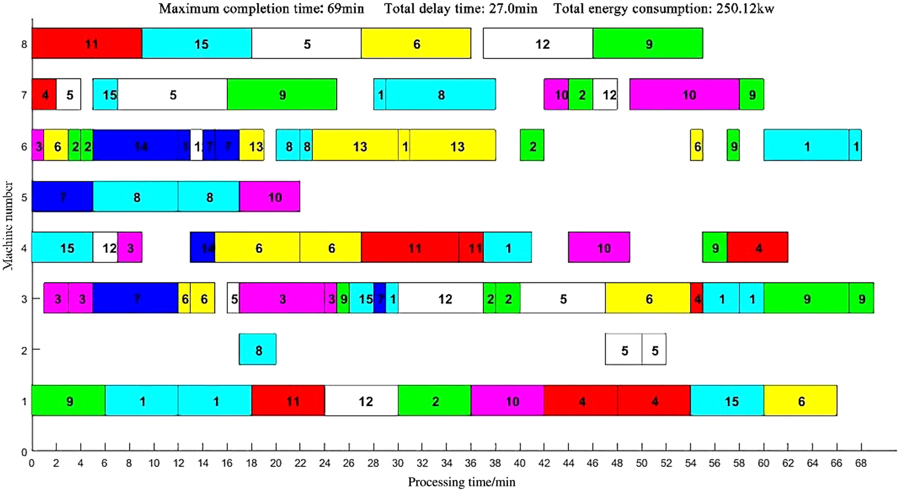
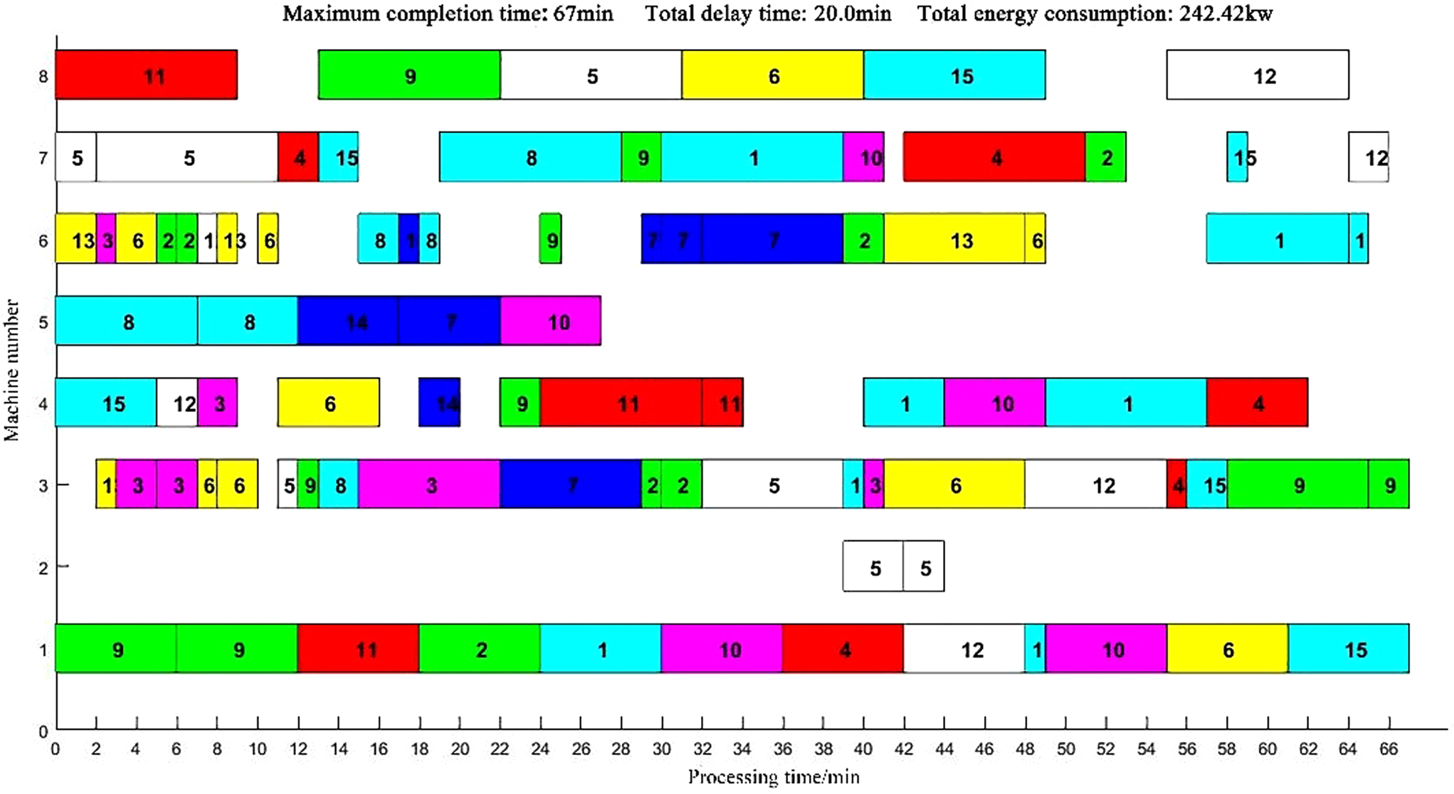
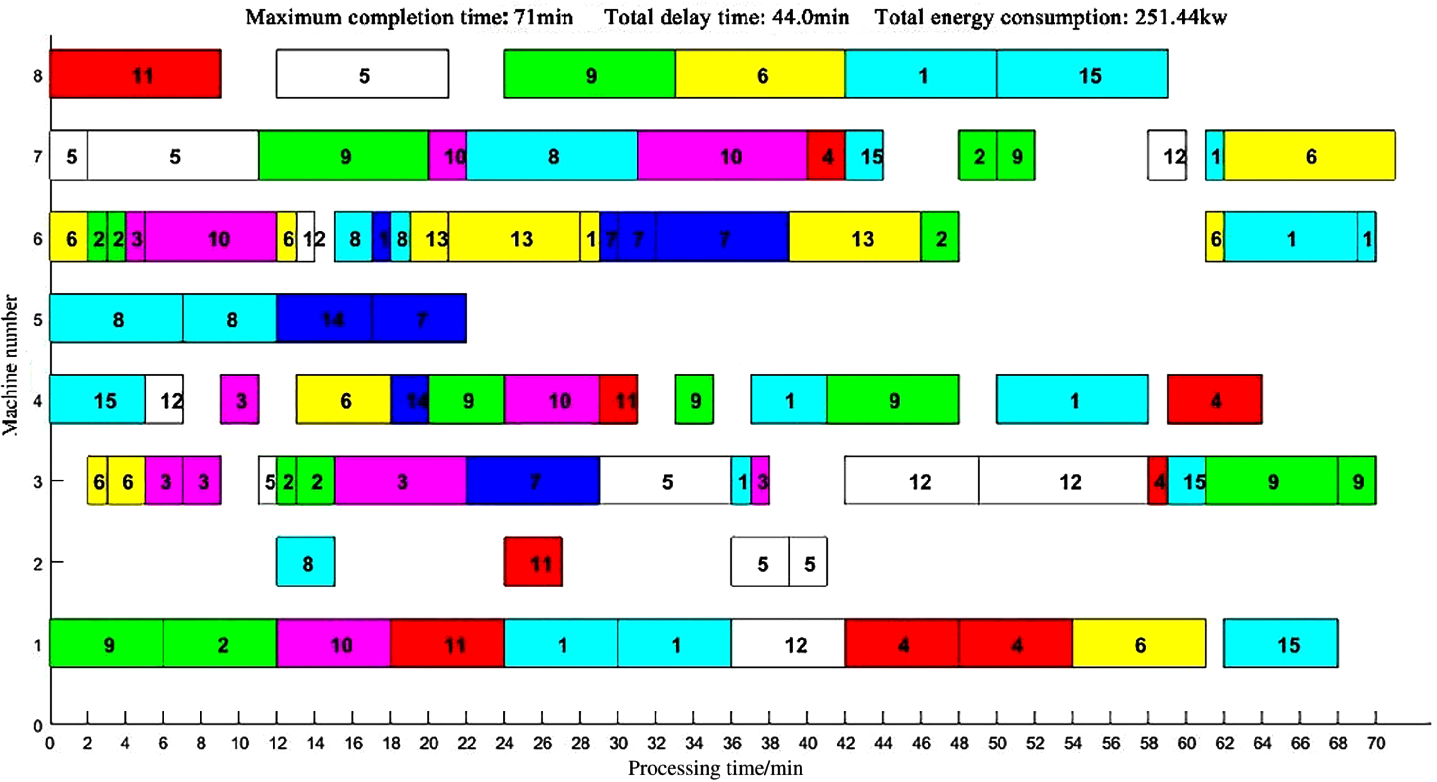
The Gantt charts of the scheduling results of the two algorithms are shown in Figs. 21–22. In terms of energy saving effect, the energy consumption of the scheduling solution obtained by CT-NSGA-II algorithm is 233.56kw, and that of NSGA-II algorithm is 242.42kw. The current scheduling method used by enterprise A is first-come-first-processed, and the energy consumption of this method is 275.8kw. The CT-NSGA-II algorithm can effectively reduce energy consumption compared with the existing scheduling method of the enterprise.

Fig. 21

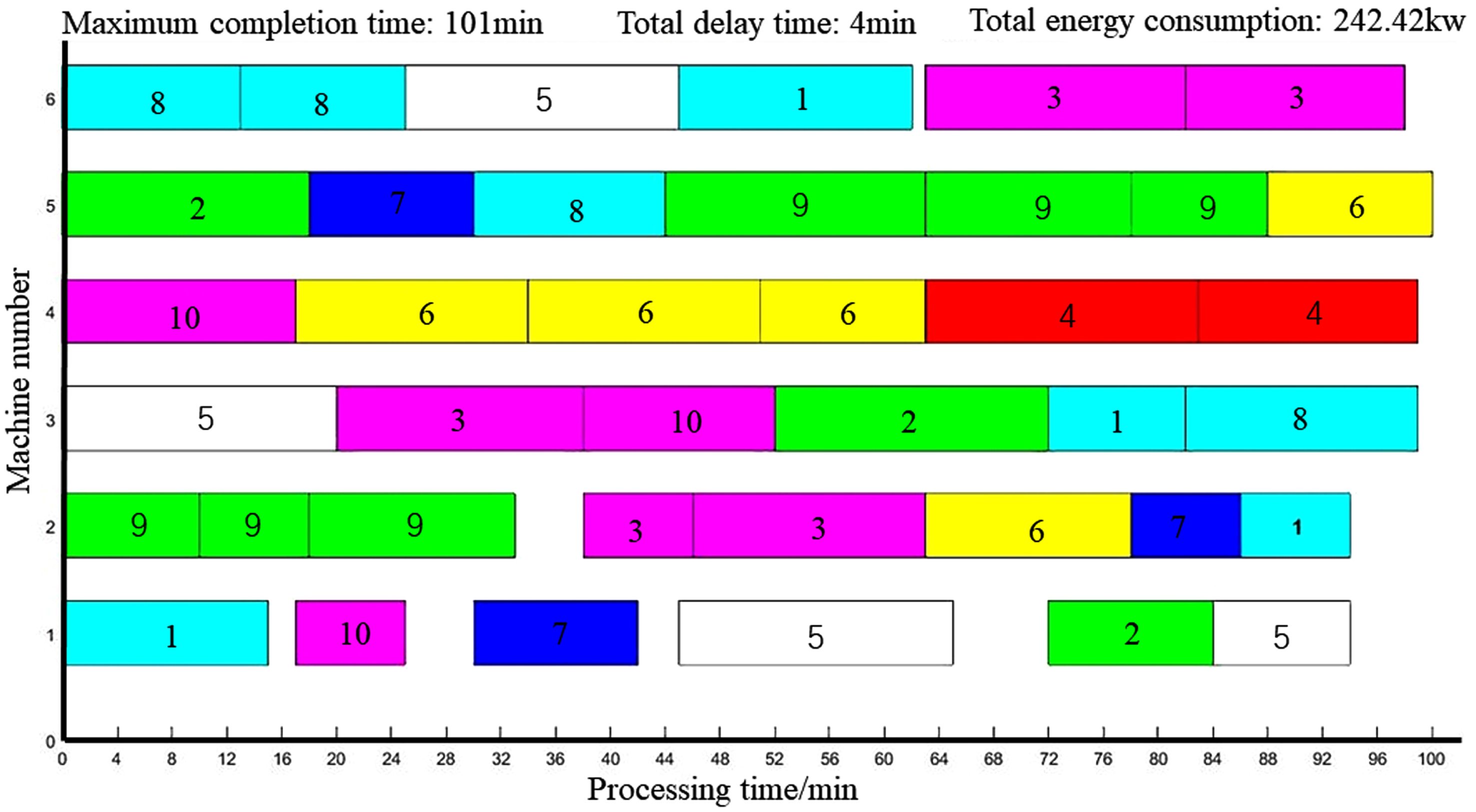
CT-NSGA-II Solving 10*6 FJSP Problem Scheduling Results Gantt Chart

Fig. 22

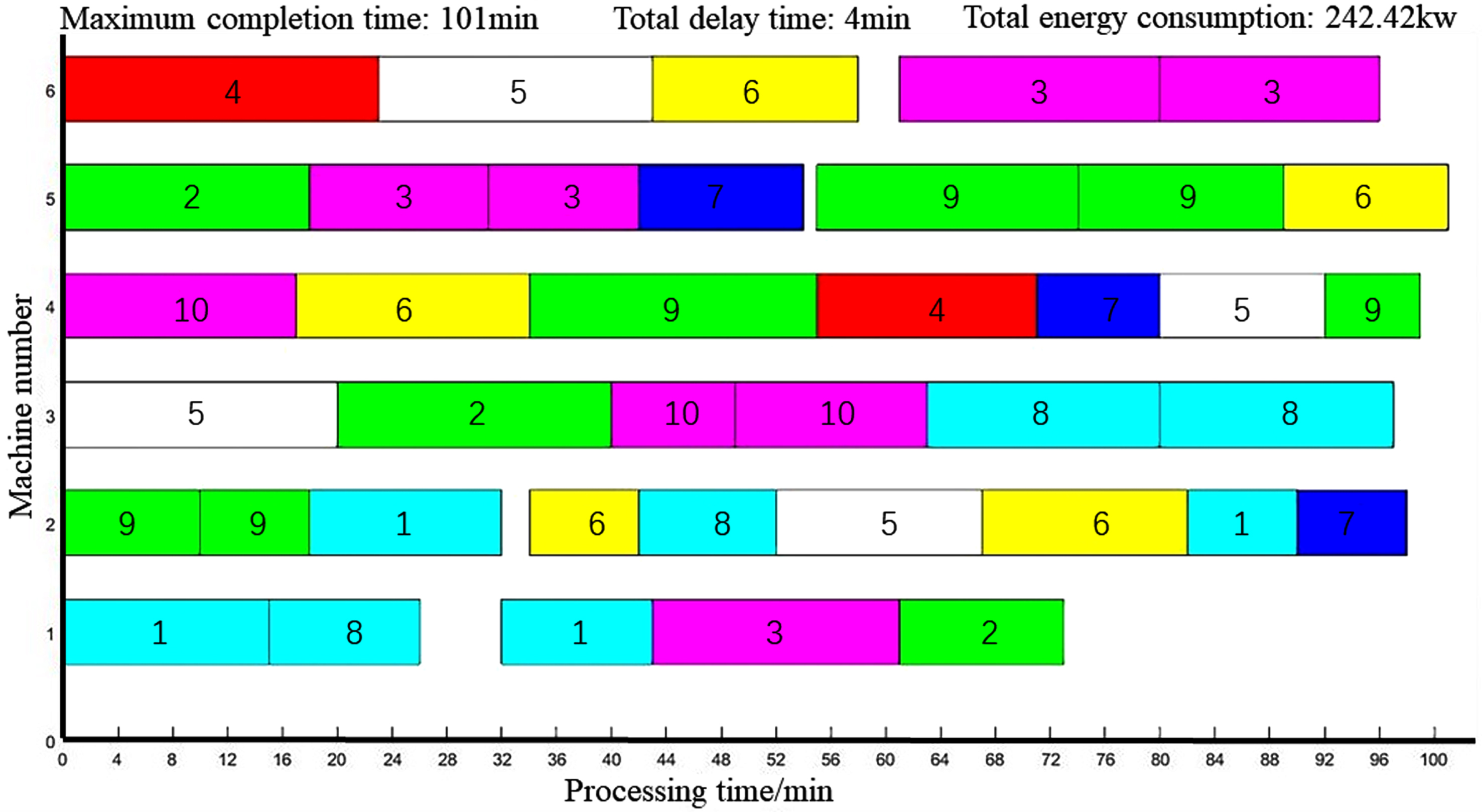
NSGA-II solving 10*6 FJSP problem scheduling results Gantt chart

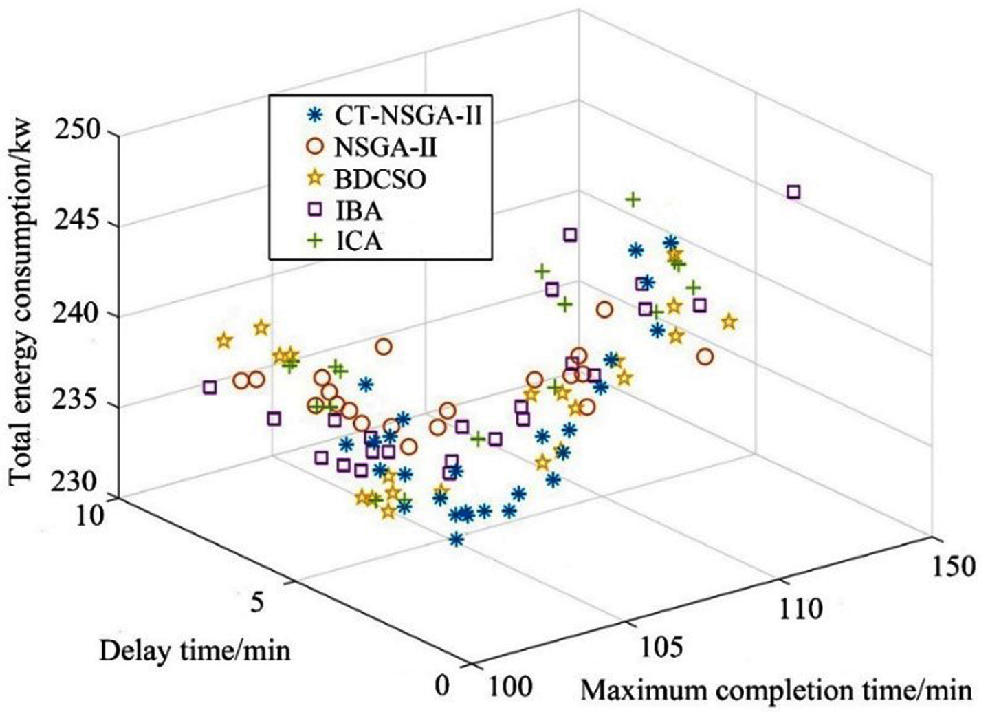
Considering the limitations of the comparison effect when solving cases with the same type of algorithms and the chance of the solution results in a single run, we added three algorithms, BDCSO [39], IBA [40], and ICA [41], to further validate the case solution based on the comparison of CT-NSGA-II and traditional NSGA-II algorithms. These three algorithms were selected because the optimization objectives of energy consumption and completion time are considered in all of them and are typical algorithms for solving the MOFJSP problem. The Taguchi method described in Section 4-A is used to calibrate the parameters of all algorithms. The final configuration of the parameters for the newly added algorithms is given in Table 12. Each algorithm was run 10 times randomly. The mean values of the corresponding performance parameters are recorded in Table 13.

Table 12

Algorithm parameters after calibration

Algorithms	Parameter	Value
BDCSO	Population size	150
	Number of iterations	1000
	Crossover probability	0.8
	Information exchange parameters	40
ICA	Population size	150
	Total number of initial empires	7
	Number of Neighborhood Searches	8
	Number of iterations	1000
IBA	Population size	200
	Pulse Loudness	0.25
	Inertia weight max/min	0.96/0.36
	Number of iterations	1200

Table 13

Comparison of CT-NSGA-II with other algorithms

Algorithms	Objective functions			Number of non-	Times (s)
	f₁/min	f₂/min	f₃/kw	dominated solutions
CT-NSGA-II	103.2	3.7	234.7	26.9	14.07
NSGA-II	105.8	3.9	243.8	20.3	12.61
BDCSO	105.4	5.4	249.6	21.8	14.27
IBA	104.5	7.2	241.8	22.3	25.24
ICA	106.3	8.6	239.5	17.4	26.79

From Table 13, we can see that CT-NSGA-II outperforms the other algorithms in terms of completion time, delay time, and energy consumption index. And CT-NSGA-II can obtain a larger number of non-dominated solutions. the running time of CT-NSGA-II is slightly longer than that of NSGA-II, which is due to the added neighborhood search strategy that increases the running time by a small amount. The Pareto fronts obtained by the five algorithms are shown in Fig. 23. the Pareto fronts of CT-NSGA-II outperform the other four algorithms in terms of convergence and diversity, and are closer to the ideal Pareto fronts.

Fig. 23

The Pareto front obtained by the five algorithms

To further compare the quality of the obtained solutions, the algorithm performance was further evaluated using the IGD and HV metrics mentioned in Section 4-C. Each algorithm is run 10 times randomly and the corresponding parameter metrics are recorded in Table 14. Where “Avg” denotes the mean value of the ten corresponding data sets.

Table 14

Performance metrics of the five algorithms

Number of	CT-NSGA-II		NSGA-II		BDCSO		IBA		ICA
times	IGD	HV	IGD	HV	IGD	HV	IGD	HV	IGD	HV
1	0.0347	1.0215	0.0359	0.9544	0.0458	0.9755	0.0498	0.9215	0.1141	0.8310
2	0.0392	1.0236	0.0567	0.9726	0.0492	0.9816	0.0482	0.8236	0.1312	0.7634
3	0.0313	1.0197	0.0332	0.8774	0.0613	0.8804	0.0511	0.9197	0.0913	0.8696
4	0.0311	1.0211	0.1003	1.0021	0.0514	1.0121	0.0432	0.9211	0.0831	0.7118
5	0.0024	1.0254	0.1145	0.8564	0.0144	0.8644	0.0464	0.7284	0.1021	0.8183
6	0.0212	1.0222	0.1100	0.9611	0.0318	0.9541	0.0558	0.8222	0.1202	0.7221
7	0.1224	1.1216	0.1236	0.8847	0.0887	0.8947	0.0544	0.9666	0.1114	0.8565
8	0.0213	1.0216	0.1425	0.7544	0.0957	0.7614	0.0311	0.7785	0.0903	0.8886
9	0.0475	1.0224	0.1540	0.8736	0.0659	0.8536	0.0574	0.9440	0.1401	0.9641
10	0.1125	1.0109	0.1478	0.8441	0.1627	0.7541	0.1266	0.9209	0.1566	1.0210
Avg	0.0465	1.0320	0.1019	0.8981	0.0667	0.8932	0.0564	0.8747	0.1140	0.8436

As can be seen in Table 14, the mean values of IGD, HV of CT-NSGA-II are the best among the five groups of algorithms, and there are nine sets of reference values that can be chosen among the ten sets of run results of IGD. The results show that the solution set obtained by CT-NSGA-II has better convergence compared to the remaining four algorithms. The combined results of Table 13, Table 14, and Fig. 23 are sufficient to prove the superiority of CT-NSGA-II among the five algorithms. This algorithm enhances the balance between convergence and diversity and improves the quality of the Pareto solution set

5 Summary

In this paper, a multi-objective flexible job shop scheduling model with maximum completion time, total delay time, and total energy consumption of the system as optimization objectives is constructed according to the actual production of flexible job shop. The model fully considers various energy consumptions of the flexible job shop on the one hand, and processing time and lead time targets on the other. A CT-NSGA-II solution algorithm is proposed for the constructed model, which generates a higher quality initial population by a GLR hybrid initialization method. The sparsity theory is introduced to perform two different neighborhood search operations on sparse solutions, which increases the diversity of the new generation population and improves the ability of the algorithm to jump out of the local optimum, and then a more comprehensive set of Pareto optimal solutions can be obtained. Finally, the competitive selection strategy is applied to select the optimal compromise solution from the Pareto optimal solution set. The correctness of the constructed model and the effectiveness of the proposed algorithm are verified through the simulation solutions of the standard and enterprise cases. In future work, the following directions deserve further research:

In the next research, the parameter selection and implementation steps of the algorithm can be further improved to achieve better optimization results, while the time and space complexity of the algorithm should also be considered.

The application of sparsity theory needs to be improved for the case of high-dimensional targets to improve the reliability of the algorithm.

Footnotes

Acknowledgments

This work was partially supported by the Natural Science Foundation of Hebei Province under Grant No. E2022202136.

Funding

This work was supported by the Natural Science Foundation of Hebei Province under Grant E2022202136.

Competing interests

The authors have no relevant financial or non-financial interests to disclose.

Author contributions

All authors contributed to the study conception and design. All authors commented on previous versions of the manuscript. All authors read and approved the final manuscript.

Ethical and informed consent for data used & data availability and access

The datasets generated during the current study are available from the corresponding author on reasonable request.

References

Suhaimi

, Nguyen

and Damodaran

, Lagrangian approach to minimize makespan of non-identical parallel batch processing machines, Industrial Engineering 101 (2016), 295–302.

Luo

, Dynamic scheduling for flexible job shop with new job insertions by deep reinforcement learning, Applied Soft Computing 91 (2020), 106208.

Manas Ranjan

, Mahapatra

S.S

, Ratikanta

Robust scheduling for flexible job shop problems with random machine breakdowns using a quantum behaved particle swarm optimisation, International Journal of Services and Operations Management 20(1) (2015), 1–20.

and Gu

, Two-population hybrid genetic algorithm for solving distributed flexible job shop scheduling problem with preventive maintenance, Control and Decision Making (2021), 1–8.

Xing

L.N.

, Chen

Y.W.

and Yang

K.W.J.J.o.I.M.

, An efficient search method for multi-objective flexible job shop scheduling problems, Journal of Intelligent Manufacturing 20(3) (2009), 283–293.

J.-Q.

, Pan

Q.-K.

and Liang

Y.-C.

, An effective hybrid tabu search algorithm for multi-objective flexible job-shop scheduling problems, Industrial Engineering 59(4) (2010), 647–662.

Wang

, Deng

, Jiang

and Zhang

, Multi-Objective Parallel Variable Neighborhood Search for Energy Consumption Scheduling in Blocking Flow Shops, in IEEE Access 6 (2018), 68686–68700.

Luan

F.Z.

, Wu

et al. Optimizing the low-carbon flexible job shop schedulingproblem with discrete whale optimization algorithm, Mathematics 7(8) (2019), 688.

Zhang

, Xu

L.-P.

, Li

, Zhao

and He

, Research on flexible job shop scheduling based on improved wolf pack algorithm, Journal of System Simulation (2022), 1–11.

10.

Wang

, Liu

, Li

and Kong

, Energy consumption scheduling in the flow shop based on ultra-low standby state of machine tools, Control and Decision Making 36(01) (2021), 143–151.

11.

Zhang

, Xu

, Tan

and Xu

, Energy-saving scheduling of dual-resource flexible job shop considering lead time, Journal of System Simulation (2022), 1–13.

12.

, Wang

and Gong

, Knowledge-driven modal algorithm for solving distributed green flexible scheduling, Journal of Huazhong University of Science and Technology (Natural Science Edition) 50(06) (2022), 55–60.

13.

Meng

, Ren

, Zhang

, Li

J.-Q.

, Sang

and Zhang

, MILP Modeling and Optimization of Energy-Efficient Distributed Flexible Job Shop Scheduling Problem, in IEEE Access 8 (2020), 191191–191203.

14.

J.-Q.

, Du

, Gao

K.-Z.

, Duan

P.-Y.

, Gong

D.-W.

, Pan

Q.-K.

et al. et al. A hybrid iterated greedy algorithm for a crane transportation flexible job shop problem, IEEE Transactions on Automation Science and Engineering 19(3) (2021), 2153–2170.

15.

, Chen

, Zhang

and Li

, A hybrid multi-objective evolutionary algorithm to integrate optimization of the production scheduling and imperfect cutting tool maintenance considering total energy consumption. , Journal of Cleaner Production 268 (2020), 121540.

16.

, Chen

, Gao

, Li

, Zhang

Multiobjective flexible job-shop rescheduling with new job insertion and machine preventive maintenance. IEEE Transactions on Cybernetics (2022).

17.

Yildirim

M.B.

and Mouzon

, Single-machine sustainable production planning to minimize total energy consumption and total completion time using a multiple objective genetic algorithm, IEEE Trans Eng Manage 59(4) (2012), 585–597.

18.

Liu

and Liu

, NSGA-II multi-objective optimization method for dynamic congestion of press shop scheduling, Forging Technology 46(01) (2021), 76–82.

19.

Liu

, Gu

, Luo

and Ding

, Improved NSGA-II algorithm based on loser group and hybrid coding strategy, Computer Science 46(10) (2019), 222–228.

20.

Han

, Wang

, Dong

, Ma

Improved NSGA-II algorithm for multi-objective scheduling problem in hybrid flowshop, 2017 9th International Conference on Modelling, Identification and Control (ICMIC), 2017, pp. 740–745.

21.

Guo

Z.X.

, Wong

W.K.

, Li

and Ren

, Modeling and Pareto optimization of multi-objective order scheduling problems in production planning, Industrial Engineering 64(4) (2013), 972–986.

22.

, Zhang

, Meng

and Wang

, Improved NSGA2 algorithm for solving flexible job shop scheduling problem, Combined Machine Tools and Automated Machining Technology (05) (2022), 182–186.

23.

Dong

, Xu

and Xie

, Multi-objective optimization algorithm for solving multi-flexible job shop scheduling problems, Computer Science 47(12) (2020), 239–244.

24.

Xie

, Li

and Liao

, An Improved NSGA2 Algorithm with Differential Local Search, Computer Science 40(10) (2013), 235–238+273.

25.

Zhang

, Gao

, Li

and Zhang

, Improved genetic algorithm for solving flexible job shop scheduling problem, Journal of Mechanical Engineering, 45(07) (2009), 145–151.

26.

Kalyanmoy Deb

et al. A fast and elitist multiobjective genetic algorithm: NSGA-II, IEEE Trans Evolutionary Computation 6(2) (2002).

27.

Luan Fei

et al. Enhanced NSGA-II for multi-objective energy-saving flexible job shop scheduling, , Sustainable Computing: Informatics and Systems 39 (2023).

28.

Jiang

, Xu

and Gang

, Improving the NSGA-II-DE algorithm using population expansion and sparsification strategies, Control and Decision Making 34(01) (2019), 55–62.

29.

Zhang

and Liu

, Resource allocation method for wireless sensor networks based on non-complete information game bidding, Journal of Fuzhou University (Natural Science Edition) 44(01) (2016), 45–51.

30.

Chai

, Zhou

, Liu

and Hu

, Scheduling Model for Dense Computing Grid Jobs Based on Dynamic Bidding Mechanism, Journal of East China Jiaotong University 26(02) (2009), 81–85.

31.

Wei

and Shu

, Active rent seeking for cloud services based on competitive bidding mechanism in cloud manufacturing environment, Microelectronics and Computers 29(09) (2012), 5–8+14

32.

C.V.

et al. Classification of energy consumption patterns for energy audit and machine scheduling in industrial manufacturing systems, Control 35(5) (2013), 583–592.

33.

Wang

, Ren

, Qiu

and Qiu

, A review of performance evaluation metrics for multi-objective evolutionary algorithms, Journal of Computer Science 44(08) (2021), 1590–1619.

34.

Ouyang

, Wu

, Fan

, Wang

Optimization of multi-media energy schedules for steel based on improved MOEA/D algorithm, Journal of Systems Simulation (2022), 1–11.

35.

Baker

K.R.

, Sequencing Rules and Due-Date Assignments in a Job Shop, Management Science 30(9) (1984), 1093–1104.

36.

Wei

et al. Unified Multi-Objective Genetic Algorithm for Energy Efficient Job Shop Scheduling, in, IEEE Access 9 (2021), 54542–54557.

37.

Zitzler

and Thiele

, Multiobjective evolutionary algorithms: a comparative case study and the strength pareto approach, IEEE Transactionson Evolutionary Computation 3(4) (1999), 257–271.

38.

Zhu Yi , Chen Lu , and , Multi-objective hybrid flow shop scheduling considering lead time[J], Industrial Engineering and Management 25(04) (2020), 159–165.

39.

Jiang

and Deng

, Optimizing the Low-Carbon Flexible Job Shop Scheduling Problem Considering Energy Consumption, in IEEE Access 6 (2018), 46346–46355.

40.

Bao

and Xu

, Multi-objective flexible job shop scheduling for energy-consumption-oriented mechanism, Computer Application Research 34(12) (2017), 3617–3622.

41.

and Lei

, High-dimensional multi-objective flexible job shop scheduling based on a novel imperial competition algorithm, Control Theory and Applications 36(06) (2019), 893–901.

Study on flexible job shop scheduling problem considering energy saving

Abstract

Keywords

1 Introduction

2 Problem description and model construction

Table 3 The values of the five parameters Parameters Level value 1 2 3 4 N 50 100 150 200 P c 0.6 0.7 0.8 0.9 P m 0.05 0.1 0.15 0.2 t max 500 800 1000 1200 k 0.1 0.15 0.2 0.25

Footnotes

Acknowledgments

Funding

Competing interests

Author contributions

Ethical and informed consent for data used & data availability and access

References

Table 3
The values of the five parameters

Parameters Level value

1 2 3 4

N 50 100 150 200

P_c 0.6 0.7 0.8 0.9

P_m 0.05 0.1 0.15 0.2

t_max 500 800 1000 1200

k 0.1 0.15 0.2 0.25