
Abstract
In the modern world, condition monitoring is crucial to the predictive maintenance of machinery. Gearboxes are widely used in machineries and auto motives to achieve the variable speeds. The major problem in gearbox is catastrophic failure due to heavy loads, corrosion and erosion, results in economic loss and creates high safety risks. So, it is necessary to provide condition monitoring technique to detect and diagnose failures, to achieve cost benefits to industry. The main purpose of this study to use Machine Learning (ML) algorithms and Artificial Neural Network (ANN) which are very powerful and reliable tool for fault detection and its most important attribute is its ability to efficiently detect non-stationary, non-periodic, transient features of the vibration signal. To do the vibration study, an experimental setup was created, and various faults were induced faults of various kinds that usually occurred in the gearbox. The gear in the gear train was subjected to vibration analysis which was captured via a sensor. Signal processing was carried out using MATLAB Toolbox. To automatically identify the flaws in the helical gearbox, an artificial neural network (ANN) and several machines learning methods, including KNN, decision tree, random forest, and SMV, were trained by creating a database from the experiment conducted. The outcomes showed potential in accurately classifying the faults. The results show that ANN has the highest accuracy of 99.6% with a 6.5662 seconds computational time while SVM has the lowest accuracy of 96% among them along with the highest computational time of 21.324 seconds.
Keywords
List of symbols and abbreviations
GMF Gear Meshing Frequency
EMD Empirical Mode Decomposition
IMF Intrinsic Mode Function
FFT Fast Fourier Transform
ANN Artificial Neural Network
KNNK Nearest Neighbor
EMD Electric Discharge Machining
DFT Discrete Fourier Transform
RMS Root Mean Square
MRMR Maximum Relevance –Minimum Redundancy
ROC Receiver Operating Characteristics
SCG Scaled Conjugate Gradient
R union of both rational and irrational numbers,
y the variable or data variable of the data set,
∑ denote a sum of multiple terms
y max highest value of the data set
y min lowest value of the data
|yi| (Modulus) value describes the distance from zero that a number is on the number line, without considering direction.
R is defined as the union of both rational and irrational numbers,
σ Standard Deviation
Introduction
Motivation and incitement
Since the discovery of gears, this tool for transmitting motion and torque from one mechanical component to another has evolved into the foundation of several machined components. It is utilized for power transmission in practically all technical applications. The gear’s design is determined depending on the industry’s distinct operational requirements.
In gears, frequent flaws include wear, pitting, impact, fatigue, tooth bending or breaking, and plastic deformation. A cracked tooth is the most frequent reason for failure among these failures. These problems may happen for a variety of reasons, including severe load transmissions, natural wear, and tear, or operational circumstances. Gears may be deemed to be defective if the gear train does not adhere to the specified design specifications, is improperly constructed or misaligned, an excessive load is applied, the material or heat treatment was chosen wrong, or accidental stresses are raised in crucial locations.
Due to the critical function that gears play in industries, their failure will result in significant production losses and process disturbance. As a result, ongoing machine health monitoring is essential for operation. Prognostics and health conditioning of all important machining components is a new branch of study that has emerged to address and prevent such production process disturbance. The creation of health indicators, which aid in tracking the system’s current health. Further analysis can be performed to determine whether or not defects are present using the input provided by the sensors. Next analyzing these factors aids in planning the maintenance schedule, replacement time, and cost appropriately. Prognostics of usable life will allow the engineers to be ready with the spare parts before time and so decrease the overall downtime in the industry by a significant share.
Literature review and research gaps
Numerous properties were identified from vibrational signals collected by the sensors, and on the basis of these features, the parameters were suggested for use. For condition monitoring, authors like Amarnath et al. [1] studied techniques like ANNs (Artificial Neural Networks) and SVMs (Support Vector Machines). Based on how the data’s root mean square, kurtosis, variance, and skewness were defined, vibrations and sound signals were measured and analyzed. In contrast to input with vibration data, the ANN approach used on the sound signals produced better results in the categorization of gear faults. Compared to the multiclass SVM-based technique used with vibration data produced better results. In contrast, Samanta et al. [2] conducted a comparison of support vector machines and artificial neural networks for fault identification. In this work, trained ANN and SVM were used to forecast defects, and the findings showed that SVM had superior accuracy and required less training time than ANN.
The benefits of utilizing deep learning models for gear fault detection have been supported by numerous studies. Researchers [3–5] talked about strategies to enhance parameter selection and model training. A deep learning model needs a lot of data to be trained, which was not always the case. Using numerical simulation and a generative adversarial network (GAN), Gao et al. [4] created a novel technique to increase the data sample set. Numerical simulations are used to generate fault samples, which are then combined with actual fault data and put into a generative adversarial network (GAN) to create synthetic fault samples. This method can be used to find errors in data samples that are incomplete, according to further research on these data. Liang et al. [3] developed a semi-supervised model which can use partially labeled data for training models using GAN.
Researchers [1, 2] conducted a comparative study between ANN and support vector machine for fault detection using vibration signals. Ümütlü RC et al. [6] developed an ANN to detect and classify the level of pitting fault in the helical gearbox. Using the cuckoo search algorithm Lin et al. [7] developed a probabilistic neural network for fault detection and found that this PNN outperforms regular neural networks. Wu et al. [8] developed a signal monitoring system based on the sound signals from the gearbox. The authors tested the PNN and back-propagation neural network. Kane et al. [9] performed a similar study by using psychoacoustic features of sound for training an ANN. Yang et al. [10] used pre-processed signals using wavelet packet transform to train ANN and genetic algorithm (GN) for fault detection. Hameed et al. [11] compared ANN and Fuzzy classifiers for fault detection.
Li et al. [12] developed a method to detect gear pitting faults, using vibration and acoustic emission signal data. The authors developed the CNN model and gated recurrent unit network for classification purposes. Liu et al. [13] developed a method to detect faults developed during the grinding process. Mohamad et al. developed a deep-learning model using a combination of CNN and LSTM networks for fault detection in helical gearboxes. Patil et al. [14] suggested fault detection method based on a transfer learning Network where a pre-trained YAMNet network is used for predictions. Tang et al. [15] developed a fault detection mechanism using transfer learning and CNN. Senanyaka et al. [16] proposed a method to visualize the learning features of the CNN filter. Wang et al. [17] proposed a method based on a multi-sensor spectrogram and modified CNN for fault detection in a wind turbine. Li et al. [18] proposed a method for fault detection under high speed and heavy loading conditions using a multi-scale multi-sensor feature fusion convolutional neural network (MSMFCNN) model.
Nie et al. [19] developed a framework based on Recurrent Neural Network to remove noisy transition matrix. Li et al. [20] proposed an LSTM model to detect early gear pitting faults. Using RNN Peng et al. [21] proposed a health index prediction and maintenance scheduling method. Wang et al. [22] performed a comparative study between CNN, RNN, and SVM. For calculating remaining useful life Caceres et al. [23] proposed a probabilistic Bayesian RNN layer model.
According to studies conducted by various authors, both support vector machines and artificial neural networks show promising results in identifying gear faults. Many experts were discussed methods like ANN (Artificial Neural Networks) and SVM (Support Vector Machines) for condition monitoring. Vibrations and sound signals were measured and analyzed based on which root mean square, kurtosis, variance, and skewness were defined from the vibration data. ANN method implemented on the sound signals showed better results in the gear fault classification rather than input with vibration data. On the other hand, vibration data yielded better results with help of the multiclass strategy of SVM based method. Further, authors were made a comparative study on fault detection using artificial neural networks and support vector machines. Trained ANN and SVM are used to predict fault and the results of this study have shown that the accuracy of ANN was better than SVM.
The various methods discussed have various advantages and disadvantages such as Artificial Neural Networks (ANN) has flexibility, it can model intricate relationships within the data and is proficient in learning from large and unstructured datasets along with this it can handle non-liner relationships across the data although it requires a lot of data in order to improve accuracy. Then SVM models have mechanisms to regulate overfitting, like regularization and kernel trick. But unfortunately picking the suitable kernel and tuning hyperparameters is a challenging task also SVM models are computationally demanding and will take large amounts of processing time for large data sets.
Decision tress can be easily interpreted and visualized and can also work with non-liner relationships in data, but this model tends to over fit. Any small changes in the data caused instability and also complex relationships within the data are not captured by this model. Random forest is simply a combination of multiple decision trees which helps to improve generalization and reduce overfitting. But here also with increase in number of tress makes it complex and increases the computational time. KNN can handle multi class problems easily but in order to do so the proper predictions required in finding the nearest k- nearest neighbor is slow for large data sets and also the accuracy depends with noisy data and number of features in the data. Based on this we can filter out on some specific characteristics based on our data and the required output. The trade-offs will be between the models will be among interpretability, accuracy, and computational efficiency
Contributions and paper organization
This paper focuses on fault detection through vibration analysis of a two-stage helical gearbox at a constant speed with different defects induced experimentally on it. Starting with the signal collection of health gear then a gear with a crack on the edge, then wear out of a small section on the hub, half of the tooth was removed, then the whole tooth was removed, and finally, two whole teeth were removed. After the data collection, the data was processed in MATLAB. Then the processed and sorted data was forwarded to different training models for model training, testing and validation.
The paper organization is as follows - Introduction Description of the experimental setup and the procedure followed for the experiment The mathematical description of the gear meshing frequency Discussion about the signal processing methods Choosing the final features based on algorithms and feature affects Training of the data collected from the experiment Discussion about results and conclusion
The initial setup was constructed in the machining lab as seen in Section 2. After mounting the gearbox, the shaft, and the motor the calibration of the overall setup was verified and later rubber sheets of 6 mm thickness were added in order to dampen any vibrations from the base of the setup. Next, the setup was moved to the noise and vibrations lab where the experiment was conducted. An IEPE sensor was attached on top of the two-stage helical gearbox via hot glue and the other end was attached to a data acquisition system to retrieve data. The data was stored and compiled into Excel sheets. The data obtained was processed and filtered for further study. The signals are plotted in the time domain and then converted into the frequency domain using a fast Fourier transform (FFT). The signal duration was about 40 seconds for healthy and each of the respective defects which were experimentally induced. An artificial neural network (ANN) and various machine learning algorithms were used to detect the faults in the gearbox automatically. Figure 1 shows the flowchart of the fault diagnosis methodology.

Process Flow Chart.
Methodology
The Fig. 1(a) flow chart describes the general flow of the work that was carried out, the first step was to collect the data. A sensor fixed on the gearbox records the amplitude and time of each entry. For each case, we obtain a different set of data, and this is called the ‘time domain’ data. This data is utilized in the time-domain curve, which forms the basis for all the data processing techniques. The graph also gives an overview of the vibration pattern at a glance and therefore is a very convenient tool for us to interpret. This time domain curve was obtained with the help of MATLAB.
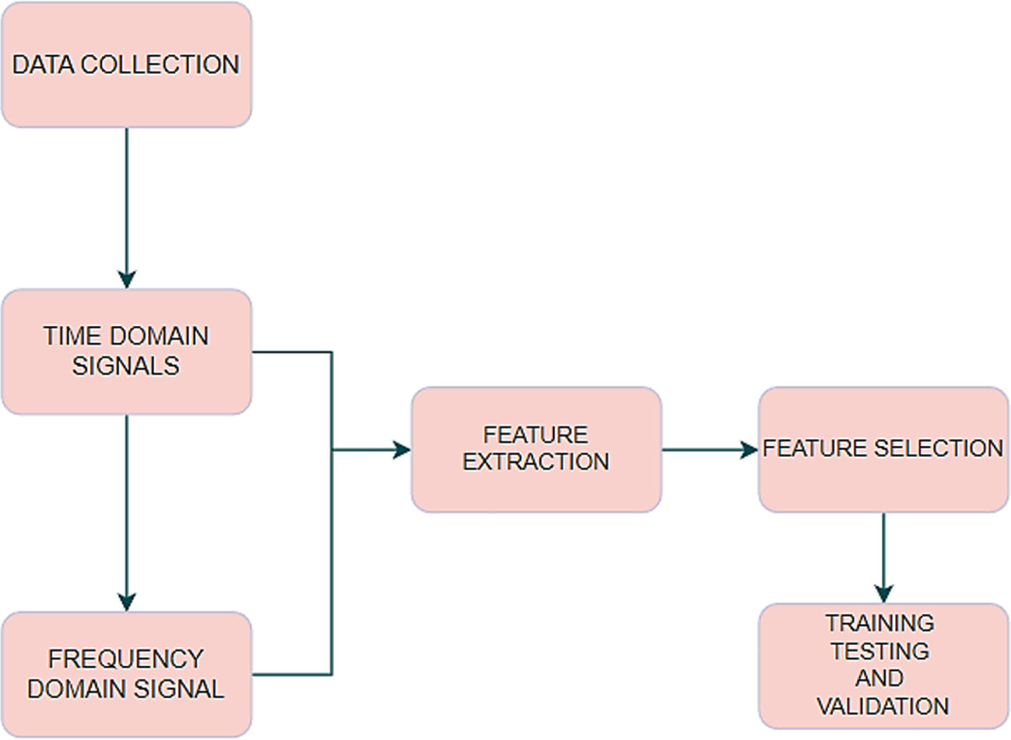
(a) Process Flow.
The vibration signals were captured using the magnetic accelerometer in the software Dewesoft and data were exported to excel for further analysis using MATLAB. Both time domain analysis and frequency domain analysis were done to study the nature of the signals. The FFT was used to extract the required frequency and amplitude. Frequency-domain curves are next, which transform the time-domain curve into a frequency-domain curve. These are mainly for easy and efficient calculations as compared to those over time-domain curves. To convert the time-domain curves into frequency-domain curves, we make use of mathematical tools in the MATLAB database. The Fourier transform technique will be utilized to transform the time domain curve to the frequency domain curve. The discrete Fourier transform (DFT) or its inverse of a sequence is calculated using a fast Fourier transform (FFT) method. A signal is transformed by Fourier analysis from its original domain, which is frequently time or space, to a representation in the frequency domain, and vice versa. This transformation helps us to read and interpret the signals.
Feature extraction is the next step, followed by the frequency-domain curves. By filtration, we are trying to get the irregularities in the signal, or in other words, we are trying to isolate the irregularities from the rest of the signals. These irregularities are characteristic of the actual vibrations in the helical gearbox and not of the machine. Thus, this gives a clearer and better picture of the vibration pattern in the gearbox.
The last and especially important step is to interpret the frequency-domain curves. Every defect will have a unique pattern of vibrations. Noting and keeping a record of these vibrations will help us identify the type of defect in the gearbox. We can compare the actual defect graphs with these experimental graphs to get an idea of what is wrong with the gearbox. The excel data were further utilized for ANN. This interpretation is done using the training models of ML algorithms and ANN, or any other modern application.
A two-stage helical gearbox with 10.5 as the gear ratio makes up as the main component in the experimental arrangement. The drive train consists of a pinion with 25 teeth followed by a helical gear of 86 teeth then a parallelly connected helical gear of 22 teeth and finally the output gear with 66 teeth. A 1-HP induction motor was connected to the gearbox’s pinion. The RPM of the motor was controlled through a voltage regulator, as shown in Fig. 2.

Experimental Setup. 1. Helical Gear Box; 2. Experimental setup base; 3. IEPE Accelerometer; 4. Shaft; 5. 1Hp Motor; 6. Rheostat; 7. Cables; 8. Data Acquisition System; 9. Data depiction.
This setup helps us record vibrational signals from the IEPE accelerometer, which are transmitted to the software with the help of cables and DAQ system integration.
The gearbox and motor were mounted on a frame covered with rubber sheets to dampen the vibrations from the frame. Based on the hole diameters present on the gearbox and the induction motor the shaft was constructed with an appropriate size of the key based on the design data book from PSG College. The 621B40 M I accelerometer type, sensor having sensitivity 1.02 mV/m/s2 and frequency range up to 12 kHz, was used in horizontal position on the gear box housing with magnetic base to collect the vibration data. The other end of the accelerometer was connected to the vibration data collector with DWESOFT software. Finally, MATLAB software was used for various signal processing.
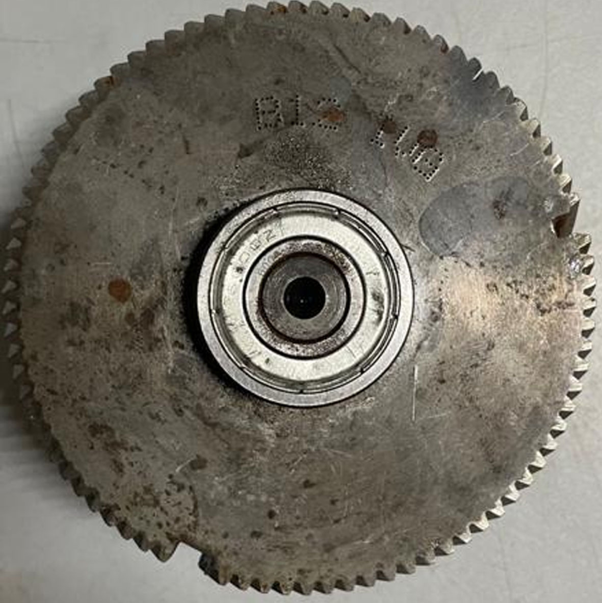
The gearbox was driven with the motor at a constant speed of 2700 rpm without any load. The vibration signals were acquired in the time domain at the sample rate of 51203 Hz for 10 s with full lubrication level in the gearbox using DEWEsoft software as shown in Fig. 6. The healthy gear can be seen in Fig. 3. Fault I is a crack of 5 mm in length and 0.5 mm in depth which was induced using spark electric discharge machining (EDM) as shown in Fig. 4. The cut depicts a crack in the gearbox brought on by dynamic loads.

Healthy Gear.
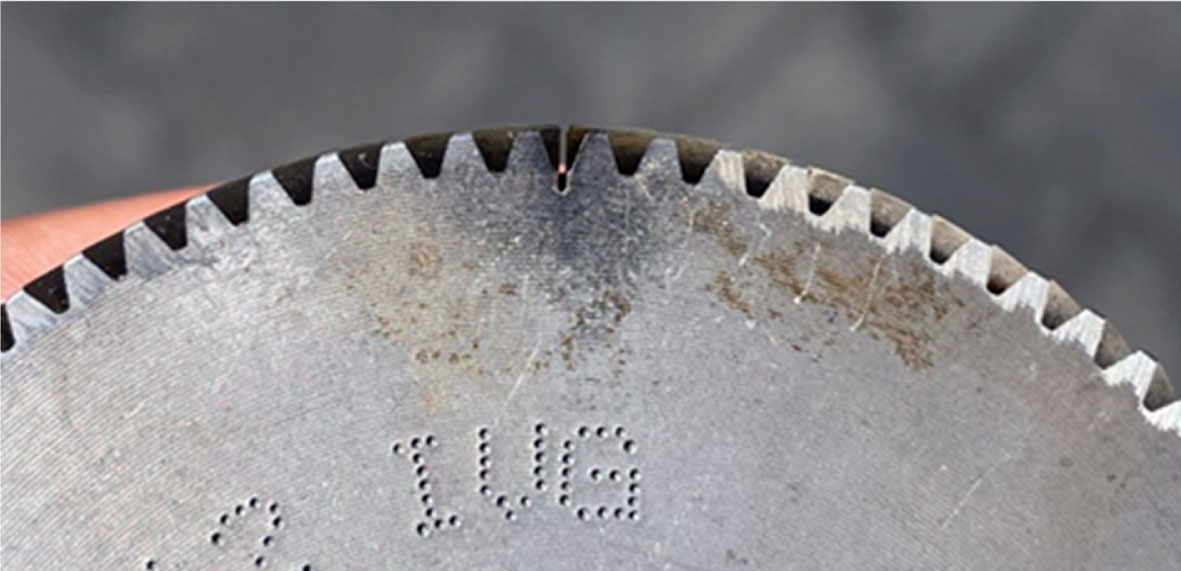
Fault I.
Fault II shown in Fig. 7 is induced by grinding a small layer on the hub of the gear to show the improper manufacturing of the gear while casting it. Fault III as seen in Fig. 5 half tooth cut on the gearwheel, as shown in. Fault IV seen in Fig. 8 is a full tooth cut on the gearwheel, as shown in and finally, Fault V shown in Fig. 9 is two whole teeth removed from the gearwheel.
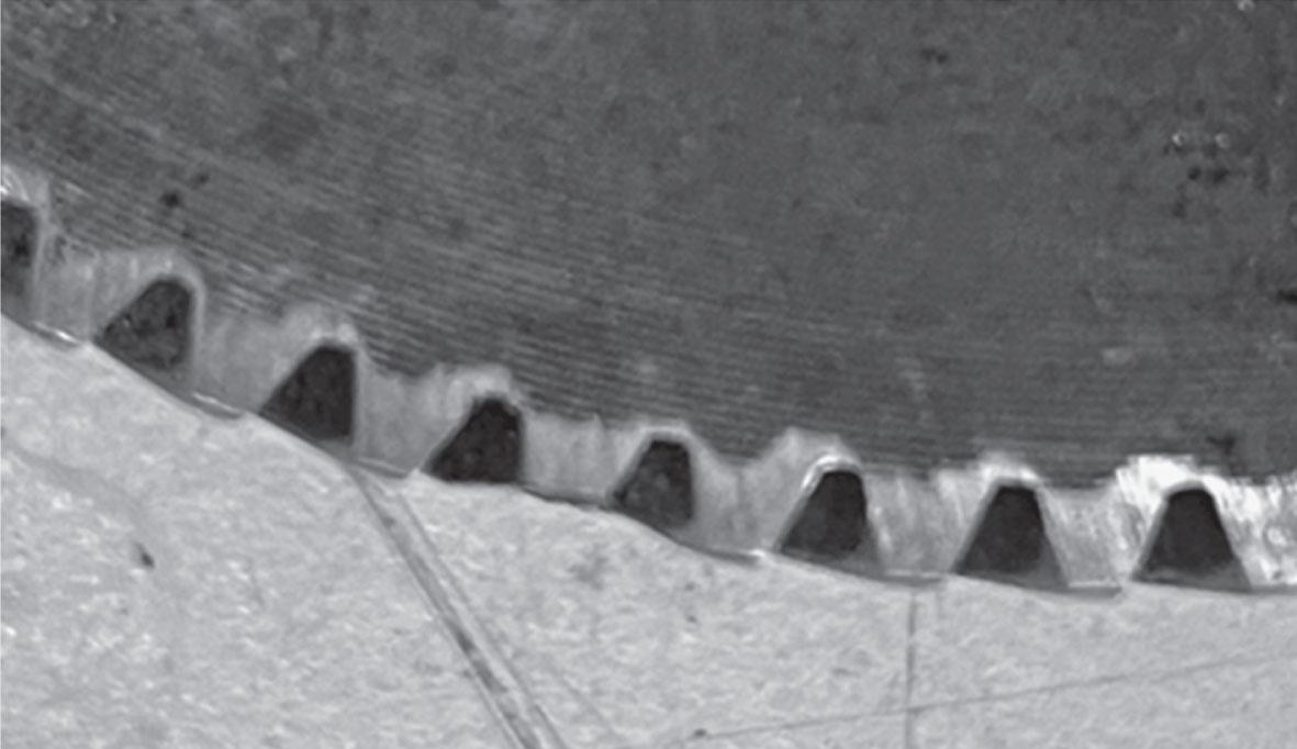
Fault III.

DEWEsoft Software.

Fault II.
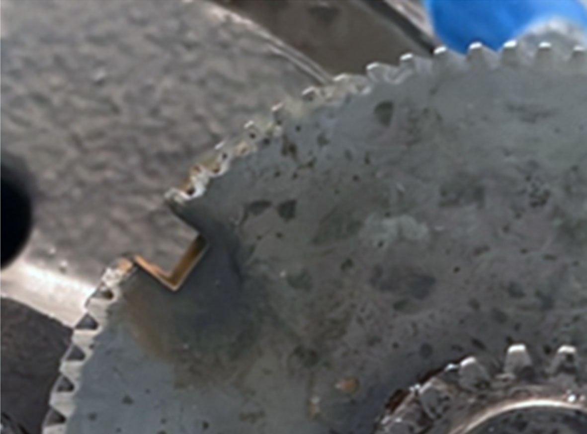
Fault IV.
Fault V.
These were also induced with the help of an electric discharge machine and generally, these types of faults occur due to the continuous running of the gearbox for a long duration of time. The signals were collected via the DEWEsoft software and then compiled into Excel files via the software for further processing. These Excel files were sorted and filtered and exported to MATLAB. The neural network toolbox was utilized to study various ML algorithms and ANN.
For a certain issue with the machinery, the vibration will be produced at a particular frequency. This data will be used to identify the problems in the machine that are causing the high vibrations. The gear mesh frequency is crucial for identifying faults.
Each gear assembly has a unique gear mesh frequency (GMF), which is present in the frequency spectrum independent of the state of the gears. The following formula is used to compute it, where T is the number of teeth and RPM is the gear’s rotational speed.
(TP –Number of Teeth in pinion, RPMP - Revolutions per minute for pinion, TG –Number of teeth in gear wheel and RMPG - Revolutions per minute for gear.
UNITS - RPM = rev/min, GMF –Hz or 1/sec)
Applying this formula in our case leads to –
For pinion:
Signal processing
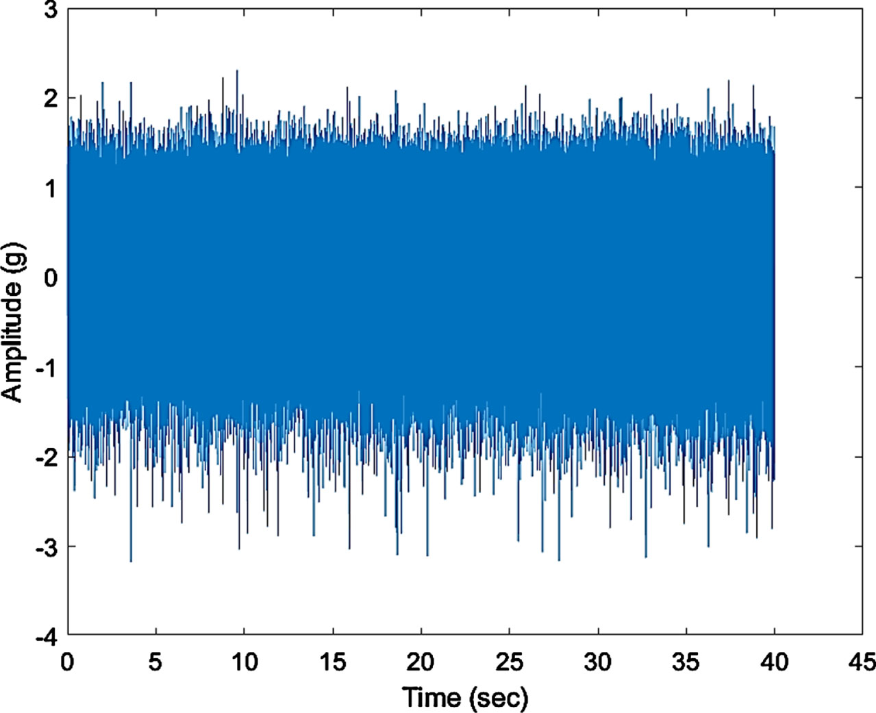
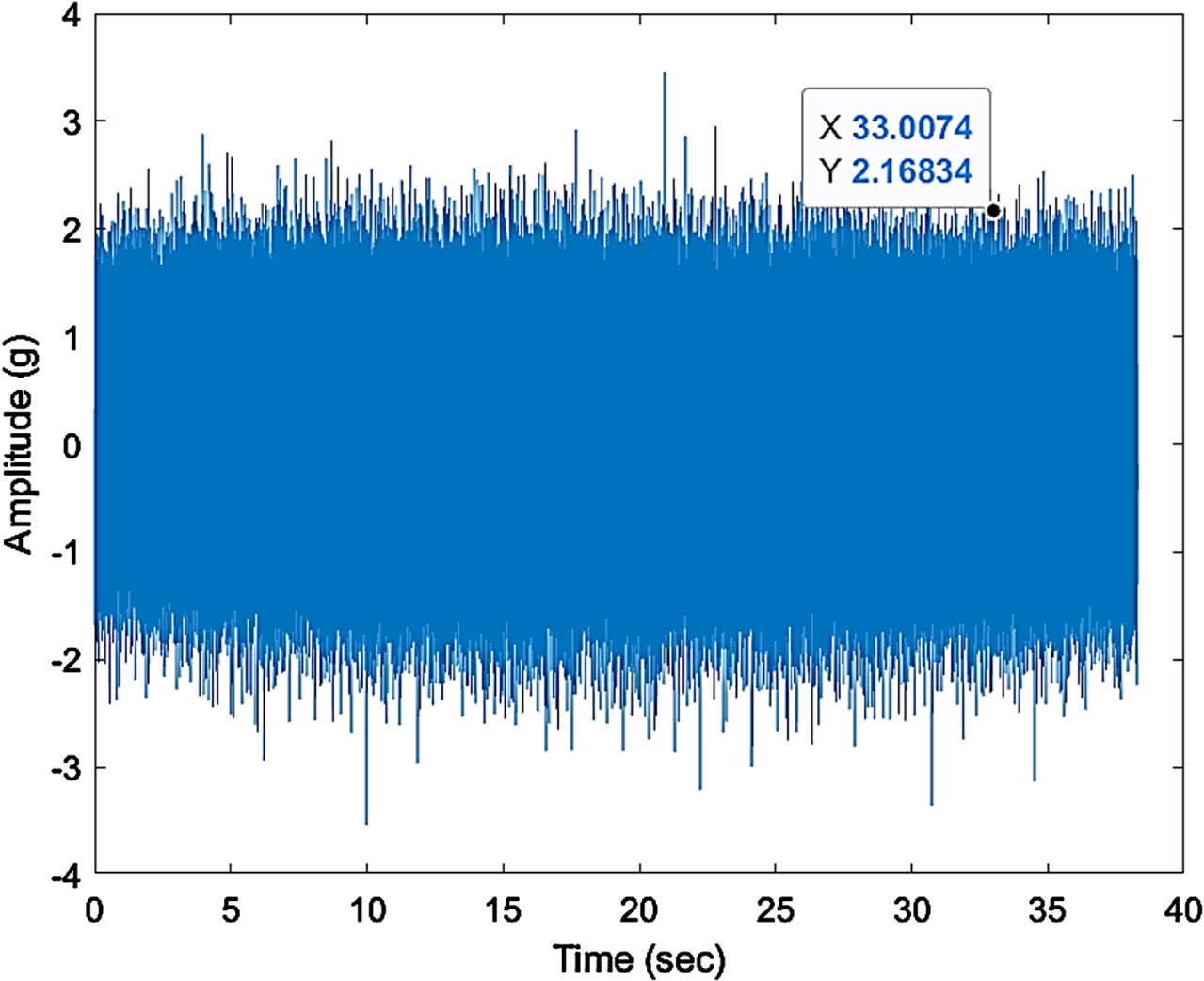
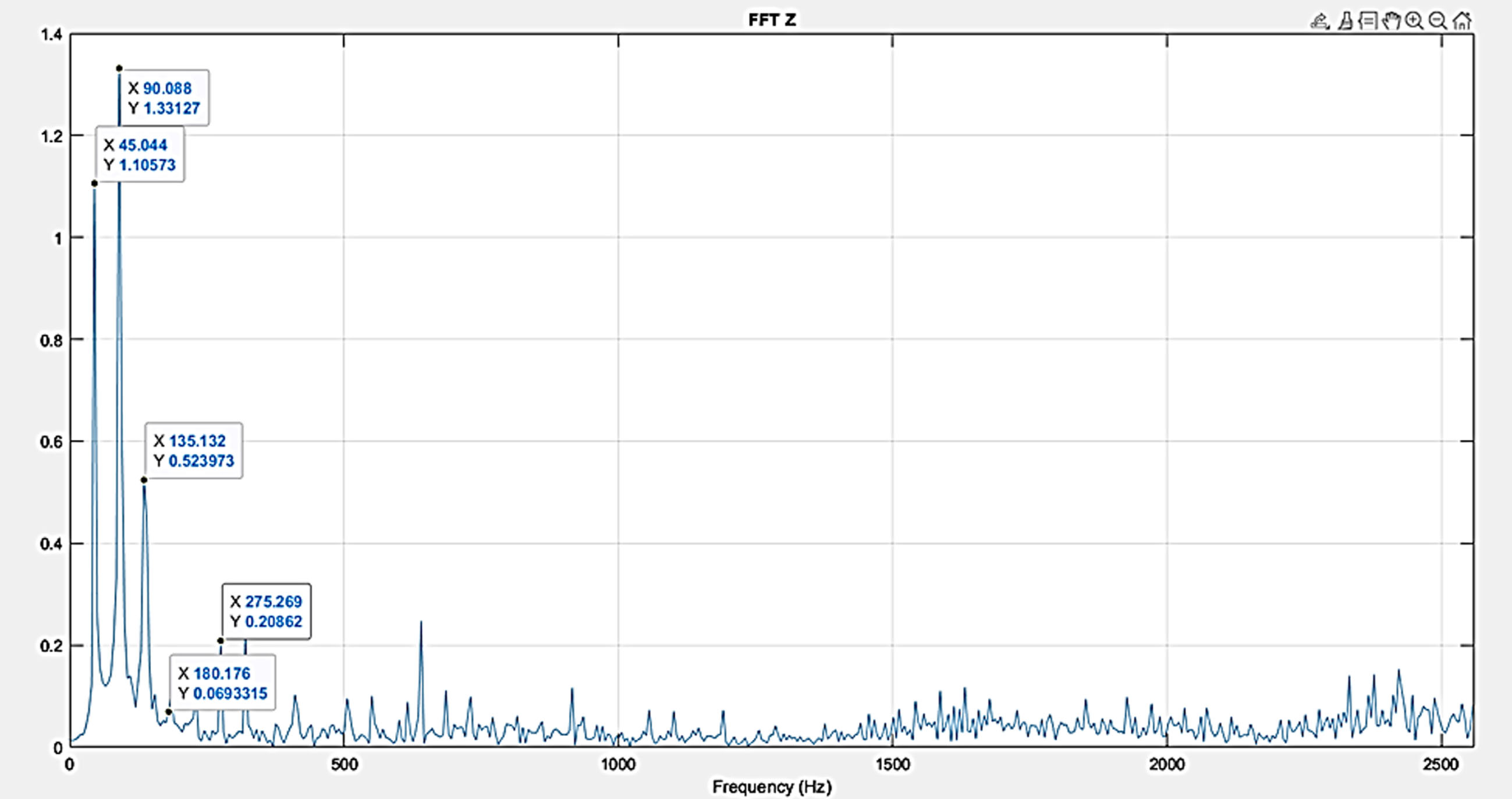
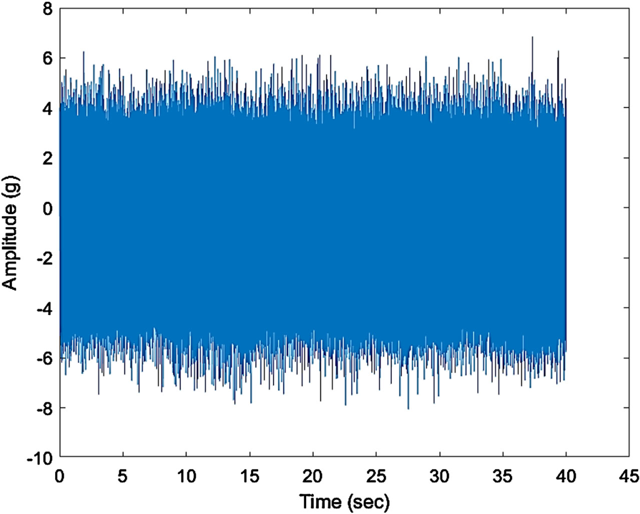
The time domain signal of a healthy gearbox is shown in Fig. 10, and the FFT is shown in Fig. 11. The highest and lowest amplitudes at a time instant can be seen from the time domain.
The motion of gear mesh frequency (GMF) was implemented to perceive the defects because GMF specifies the frequency at which the teeth on the gear and pinion come into contact with each other. The dispersal of a signal’s energy over a range of frequencies can be viewed in the frequency domain. The existence of defects can be recognized from the frequency domain by detecting the disparity of parameters like the amplitude of gear mesh frequency.
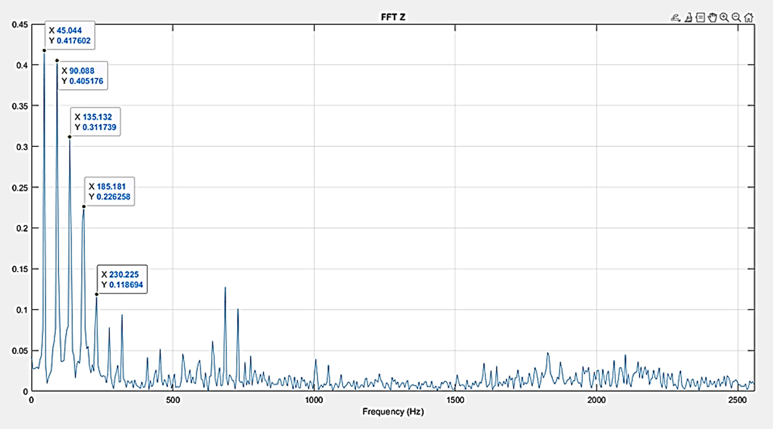
The time domain signal was converted to the frequency domain using the Fast Fourier Algorithm. The plot was frequency vs amplitude Fig. 11 shows the FFT for the healthy readings. Frequency of the gear is RPM/60 = 2700/60 = 45 Hz.
Healthy readings
From the experimental set up the raw signal data were collected and FFT was plotted and the signal processing was carried out for the healthy gears. Figure 10 shows time domain for full oil healthy condition. Figure 11 shows frequency domain for full oil healthy condition. The raw signal was collected for 10 seconds at the sampling rate of 12 000 Hz. Then readings were processed with MATLAB software to convert time versus amplitude plot. Figure 11 shows FFT raw signal for full oil healthy condition where FFT represents a natural frequency of 45 Hz and a peak amplitude of 0.417 m/s2 which is nearly corresponds to the calculated value of 45 Hz(RPM/60 = 2700 = 45) and hence the result is validated.
Time Domain Plot.
FFT plot.
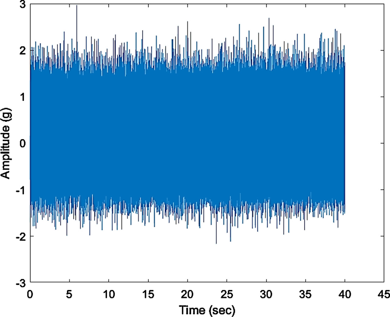
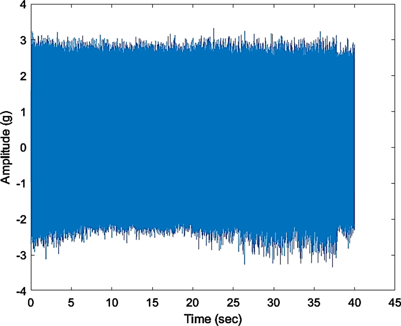
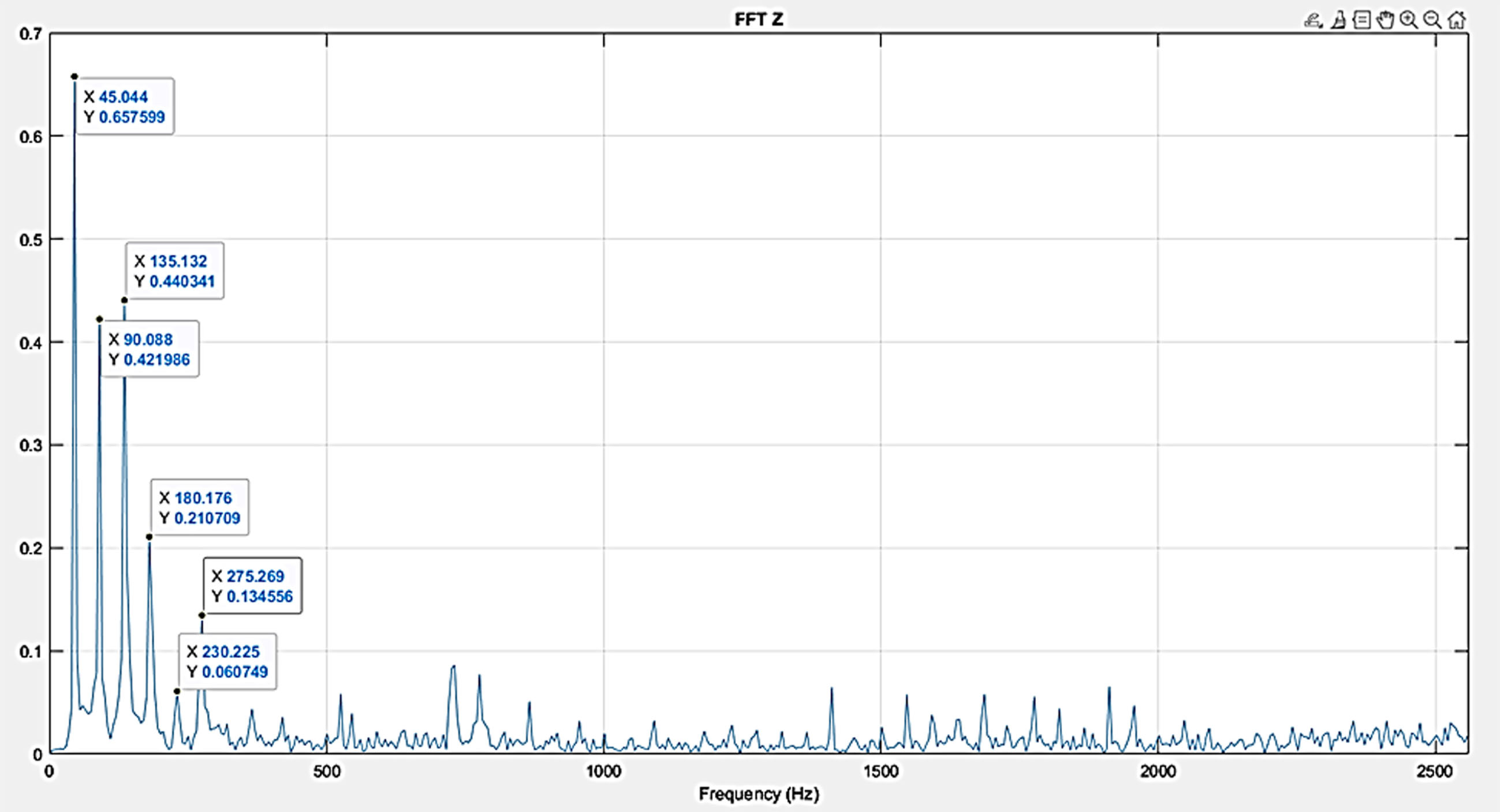
It is well known that the major components in gear vibration spectra are the tooth meshing frequency and development of harmonics, together with sidebands due to modulation phenomena. The increment in the number and amplitude of such sidebands may indicates a defect 1 condition of gear. It may acts as a tool for aiding the gear fault diagnosis on gear. Figure 12 shows time domain signals of defect 1 condition. The Fig. 13 shows frequency and its side bands are represented in various power spectrums with indication of data cursor frequency value of around 90 Hz, which crosses frequency of 45 Hz and indicates that there was existence of fault.
Time Domain Plot.

FFT plot.
Figure 14 shows time domain plot for defect 2. Figure 15 shows that there is a large increase in sideband amplitude 1.521 m/s2indicates that something changes in the geometry and is also a cause of concern. The relative amplitude of sideband to gear mesh peak is a good parameter to see in the plot. Analyze the waveform for periodic impacts that relate to rotational speed of the gears. Gear failure will permit unexpected shaft displacement thereby upsetting gear engagement. Further, tooth failure precedes gear damage.
Time domain plot.

FFT plot.
Figure 18 represent the time domain plot a gear with a tooth chip present on it respectively. Figure 17 represent the Fast Fourier transform along with the increasing amplitude of the harmonics as the intensity of the defect increases.
Time domain plot.
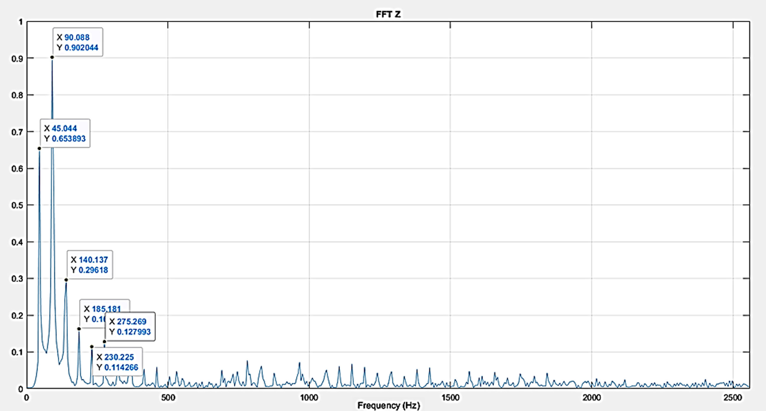
FFT plot.
Increased impacting from deterioration of gear in the transfer of power may excite gear natural frequencies. From the FFT plot, it is observed that the frequency 90 Hz and vibration amplitude of 0.902 m/s2 which crosses 45 Hz and 0.417 m/s2. This changes in the number and strength of the side bands indicate severity of fault.
Figure 18 represents the time domain plot for defect IV i.e., when one whole tooth was removed from the gear and similarly, Fig 20 represents defect V i.e., when two teeth were removed from the gear. It is observed in Figures. 19 and 21 that the Fast Fourier transforms for the plots show the increased amplitude of harmonics with the higher intensity defects.
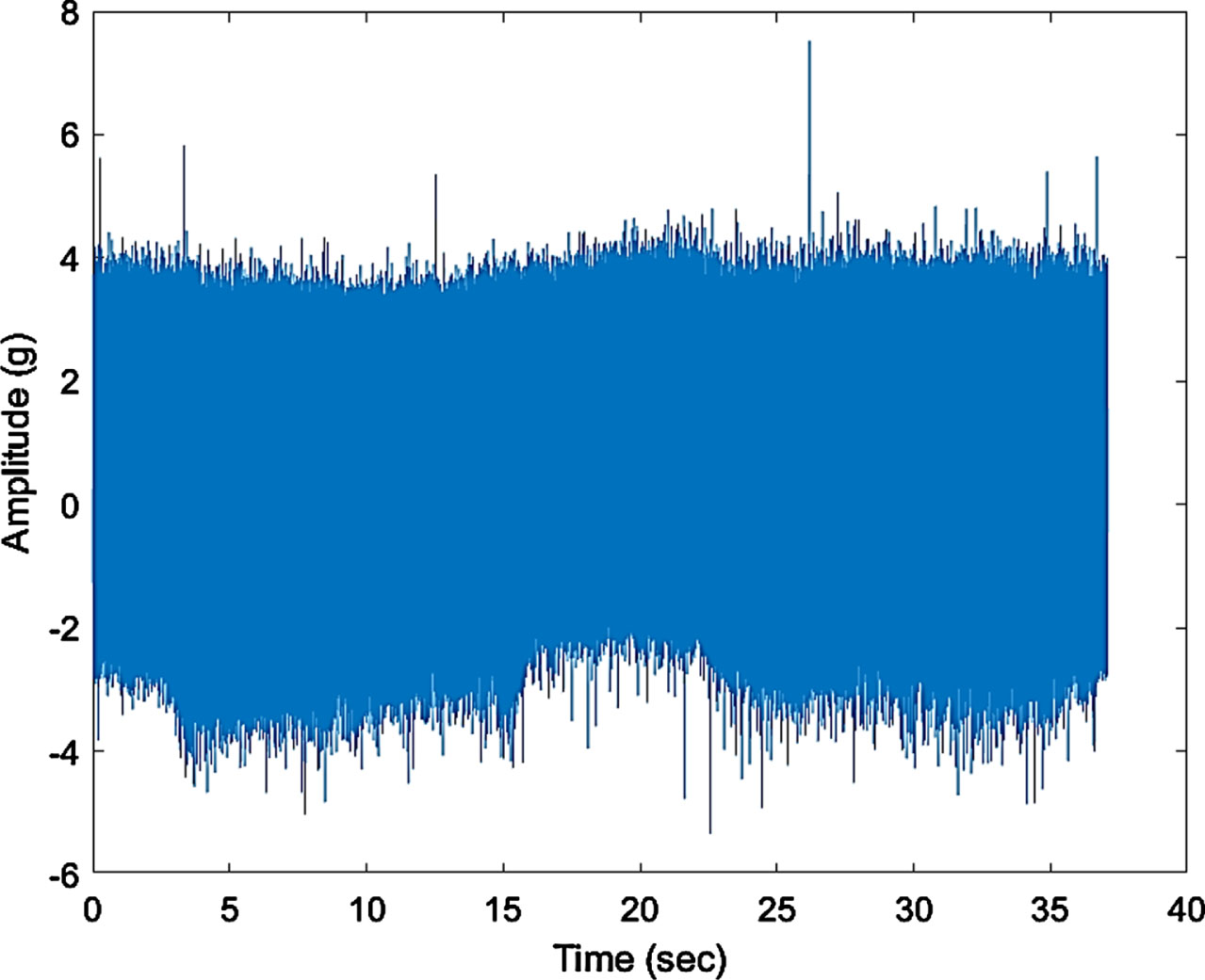
Time domain plot.
FFT plot.
Time domain plot.
FFT Plot.
These observations validate the results of indication of a fault contact within gear box. Thus, a vibration signature modulated at the rotational speed of the unit is an illustrative of a continuous fault source in the gearbox. This continuous fault implies a sustained contact between the gear tooths generating vibration levels above the operational background levels. Comparing the above spectrums it can be found that the amplitudes of the vibration, frequency and its harmonics increase with the increasing faulty conditions.
Feature extraction
Data refining and sorting are crucial for data processing and implementing proper recognition filters and parameters to utilize the data for defining other segments. In this case of huge statistical data, we need different disciplines and various parameters to sort the data and fine-tune the results. Here the statistical parameters come into the picture
1. Standard Deviation helps us understand the nature of the data on how the data and the vibration are deviating by magnitude [24].
(σ –Standard Deviation, R - union of both rational and irrational numbers, y - the variable or data variable of the data set, ∑ (sigma) is used to denote a sum of multiple terms Units - seconds)
2. RMS (Root mean square) gets us the mean line of the data which represents the data as a whole [24].
(R - union of both rational and irrational numbers, y - the variable or data variable of the data set, ∑ (sigma) is used to denote a sum of multiple terms)
3. Peak to peak represents the range of the data i.e., difference between maxima and minima [24].
(y max - highest value of the data set, y min - lowest value of the data)
4. Crest Factor helps us differentiate the extremities in a data set and understand the maximum and peak values of the data set [24].
(|yi| (Modulus) value describes the distance from zero that a number is on the number line, without considering direction.
5. Form Factor in general is a mathematical way to compare two different variables of an object by ratios. It is defined as RMS by the average of the data set [24].
6. A shape Factor equal to one gives the symmetry of the data set [24].
(R is defined as the union of both rational and irrational numbers, |yi| (Modulus) value describes the distance from zero that a number is on the number line, without considering direction)
7. Skewness gives the direction of the outliers if it is right-skewed, most of the outliers are present on the right side of the distribution while if it is left-skewed, most of the outliers will present on the left side of the distribution [24].
(R is defined as the union of both rational and irrational numbers, ∑ (sigma) is used to denote a sum of multiple terms,σ –Standard Deviation, y - the variable or data variable of the data set)
8. Margin Factor defines the limits and margin of the given data set [24].
(R is defined as the union of both rational and irrational numbers, ∑ (sigma) is used to denote a sum of multiple terms, y - the variable or data variable of the data set, |yi| (Modulus) value describes the distance from zero that a number is on the number line, without considering direction)
9. While Kurtosis measures the peak value of the data set and indicates if the signal is impulse in nature. It also helps understand the normal distribution of the data set [24].
(R is defined as the union of both rational and irrational numbers, ∑ (sigma) is used to denote a sum of multiple terms, y - the variable or data variable of the data set, σ –Standard Deviation)
10. Impulse Factor components in vibration signals are important fault features that help detect faults and their characteristics [24].
(R is defined as the union of both rational and irrational numbers, ∑ (sigma) is used to denote a sum of multiple terms, y - the variable or data variable of the data set, |yi| (Modulus) value describes the distance from zero that a number is on the number line, without considering direction)
Many algorithms are available to find feature importance scores but for our study, we are using MRMR (Maximum Relevance –Minimum Redundancy) algorithm. MRMR algorithm tries to find the minimum number of features which can classify inputs with greater accuracy [25]. The feature selection process helps to find the minimum number of features for classification, this reduces training time and increases accuracy. The MRMR algorithm finds set of features which are mutually dissimilar and can effectively represent response variable. As the name says MRMR algorithm minimizes the redundancy and maximizes relevance of feature set. The MRMR algorithm finds the pairwise mutual information using the function I(.,.) which is –
Here, X is feature set and Y is response variable Ω
Y
and Ω
X
are sample spaces corresponding to Y and X. p (x, y) is the joint probability density. p (x) is marginal density function [25]. Based on this mutual information of pairwise features algorithm finds feature importance score based on function-
Here, X i is feature is one feature, I () is mutual importance score, S is a feature set. This function iteratively calculates pairwise mutual information and selects the features with highest feature importance score f mRMR (X i ). The output of this function can help to choose important features for model training [25].
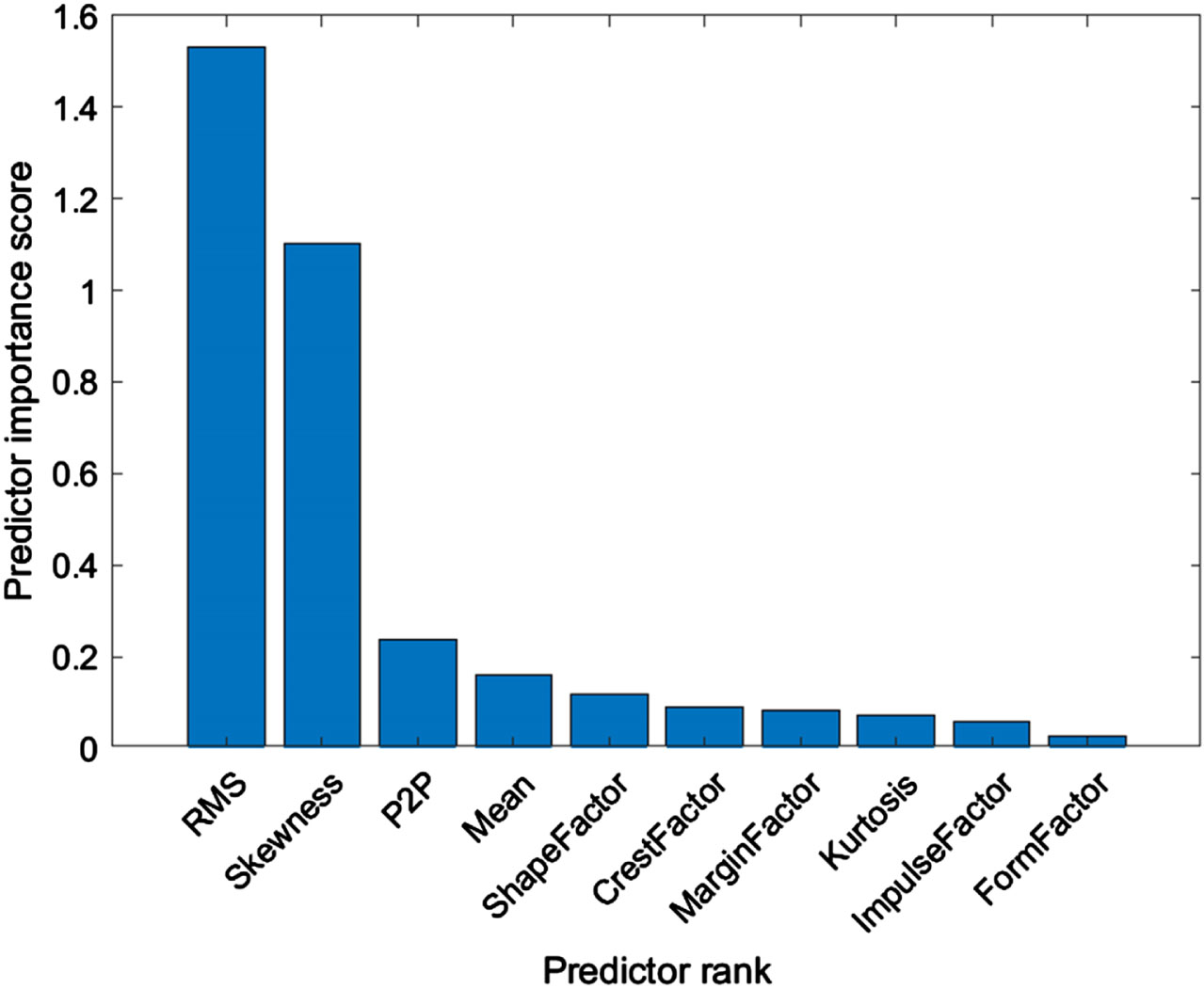
Prediction rank.
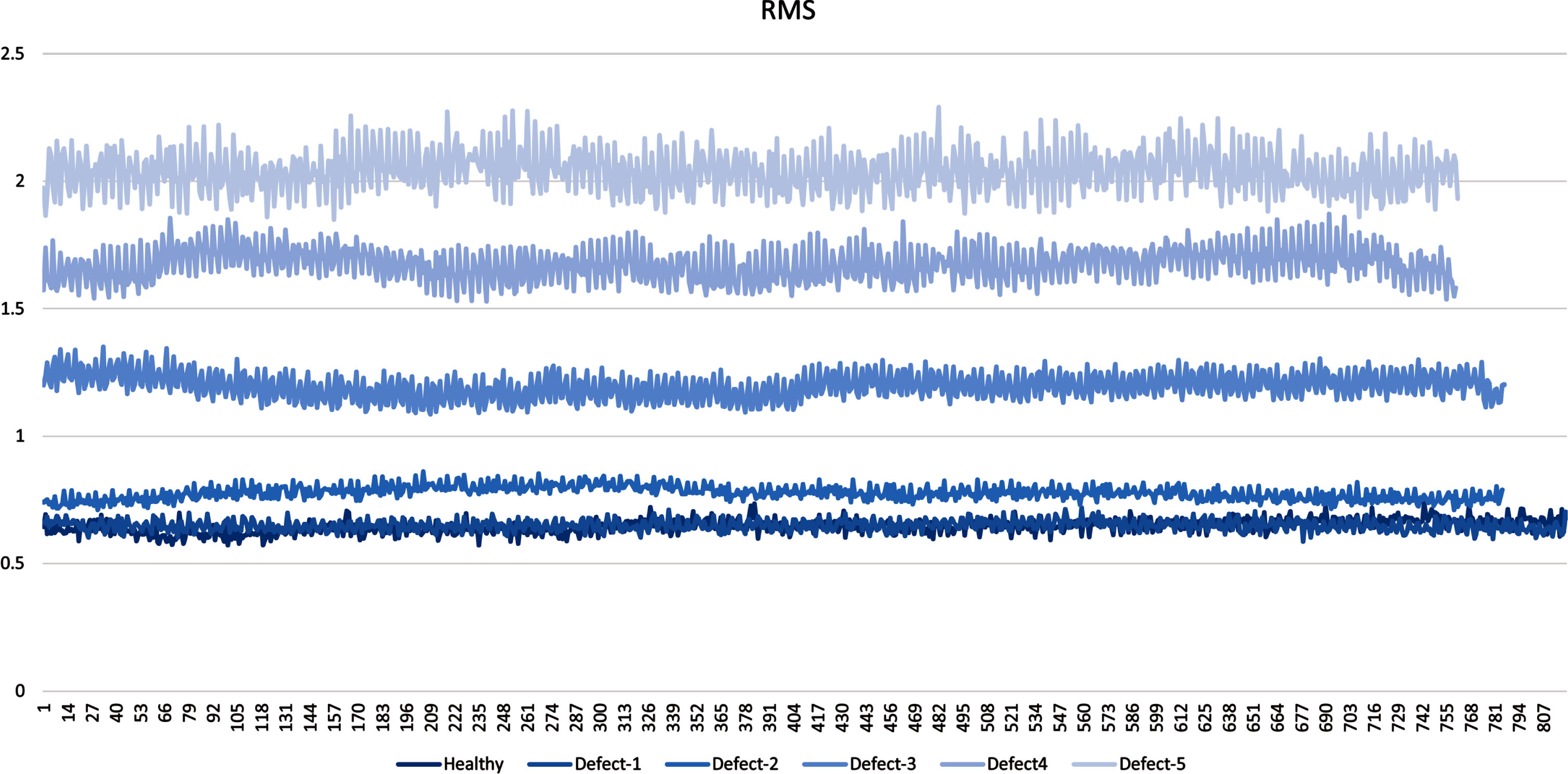
RMS PLOTS.
MATLAB software provides direct function ‘fscmrmr’ to calculate feature importance score. After using the MRMR algorithm we get the feature importance score of each feature we extracted, in our case these features are 10 statistical parameters. The output of the MRMR algorithm is shown below in Figure. From the results, we can conclude that RMS, Skewness are the most important features for classification purposes. These 2 features have more importance that other Factors.
From results of these algorithms, we can conclude that RMS is the most important parameter for classification and it can also be confirmed from plot below that we can easily classify defect based on RMS value. Other than RMS Skewness is another important parameter. For further study ae considered RMS, Skewness, P2P, Mean, kurtosis, crest factor for classification.
Support vector machine
Support vector Machine was first introduced in 1992 by Vapnik and his team [26]. Support Vector Machine or SVM models are simple supervised learning algorithms which can be used for classification purpose. This algorithm tries to find hyperparameters that can separate data points in higher dimensional vector space. SVMs are based on statistical learning theory called Structural Risk Management (SRM). The purpose of SVM algorithm is to find hyperplane which can separate different classes with maximum margin [27]. The points on class boundary are called as support vectors. In SVM for simple problem with two classes boundary which separate these classes can be represented by-
Here w is boundary and b is bias [27]. SVM classify data points using decision function-
Here x i are support vectors. In cases where linear boundary is not enough to classify classes, hyperplanes are used. This idea of using SVM to separate two classes can also be used for classification more than two classes. In cases where data is not linearly separable kernel tricks are used to convert input space into higher dimensional feature space where data is separable.
For training the model we are using RMS, Skewness, P2P, Mean, kurtosis, crest factor these 6 parameters which we found in the feature extraction step. With this input and the setting the hyperparameters we are training the SVM model.
Hyperparameters: -
For training the SVM model we need to provide some hyperparameters which are kernel function, and kernel scale. For our study, we are using a Fine Gaussian SVM kernel with a kernal scale of 0.79 which is the default in MATLAB.
Performance: -
After setting the model hyperparameters model took around 21.324 seconds for training and the model was able to attain an accuracy of 96%. Figure 24 represents the confusion matrix of trained model from this confusion matrix we can confirm that model was able to classify Healthy, Defect1, Defect II, Defect III, Defect IV and Defect V with 94.1%, 94.8%, 94.6%, 98.4%, 94.6% and 100%, accuracy. Also, the confusion matrix shows that the model classified gear with least errors of 1.6%, with error in each classification of 5.9%, 5.2%, 5.4%, 1.6 and 5.4% for healthy and respective defect gears. Figure 25 represents the receiver operating characteristics curve (ROC) which summarizes confusion matrix with different thresholds.

Confusion matrix.
ROC curve.
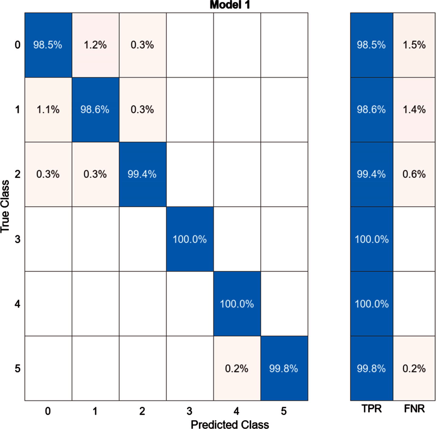
The diagonal elements color coded in blue represent the accuracies for the correctly identified reading from the training data while the peach color coded elements represent the incorrectly identified data from the readings. A vertical rectangular segment which is shown next to the confusion matric represents the cumulative true positive rate and the false negative rate for healthy and the respective defective readings. The false positive rate is when defect is not present, but the machine learning model is predicting defect is present in gear on the other hand false negative rate is when defect is present, but model is predicting defect is not present. These True positive and False Negative rates are also displayed in confusion matrix and in the ROC curve.
Decision tree models are used for both classification and regression problems. These are supervised learning algorithms that creates a tree-like structure with each possible value of features. These algorithms use divide and conquer approach for solving the problem. There are different decision tree algorithms used for classification and regression. In this study we are using CART algorithm which stands for classification and regression trees, this algorithm was introduced in 1984 by Breiman [28]. This algorithm uses binary splitting of attribute based on the gini index as splitting criteria. Gini index is an impurity-based criterion which used to measure divergence between the probability distribution of attribute values. Gini index is defined as-
For selecting the attribute evaluation criterion is defined as-
‘Here, S is training set, y is the target attribute [29].
For the training decision tree, we need to set some hyperparameters like maximum number of splits in tree, splits criteria etc.
In case of current study S is the set of 6 statistical parameters we calculated and the y is the value which represents the defect type like healthy, or defect type. As discussed earlier the data provided for the model training is labelled data. Using this labelled data and hyperparameters we trained the decision tree model.
Hyperparameters: -
For training decision tree model, we need to configure maximum number of splits and split criteria. We are using maximum 100 splits at each node and Gini’s Diversity Index as split criteria.
Performance: -
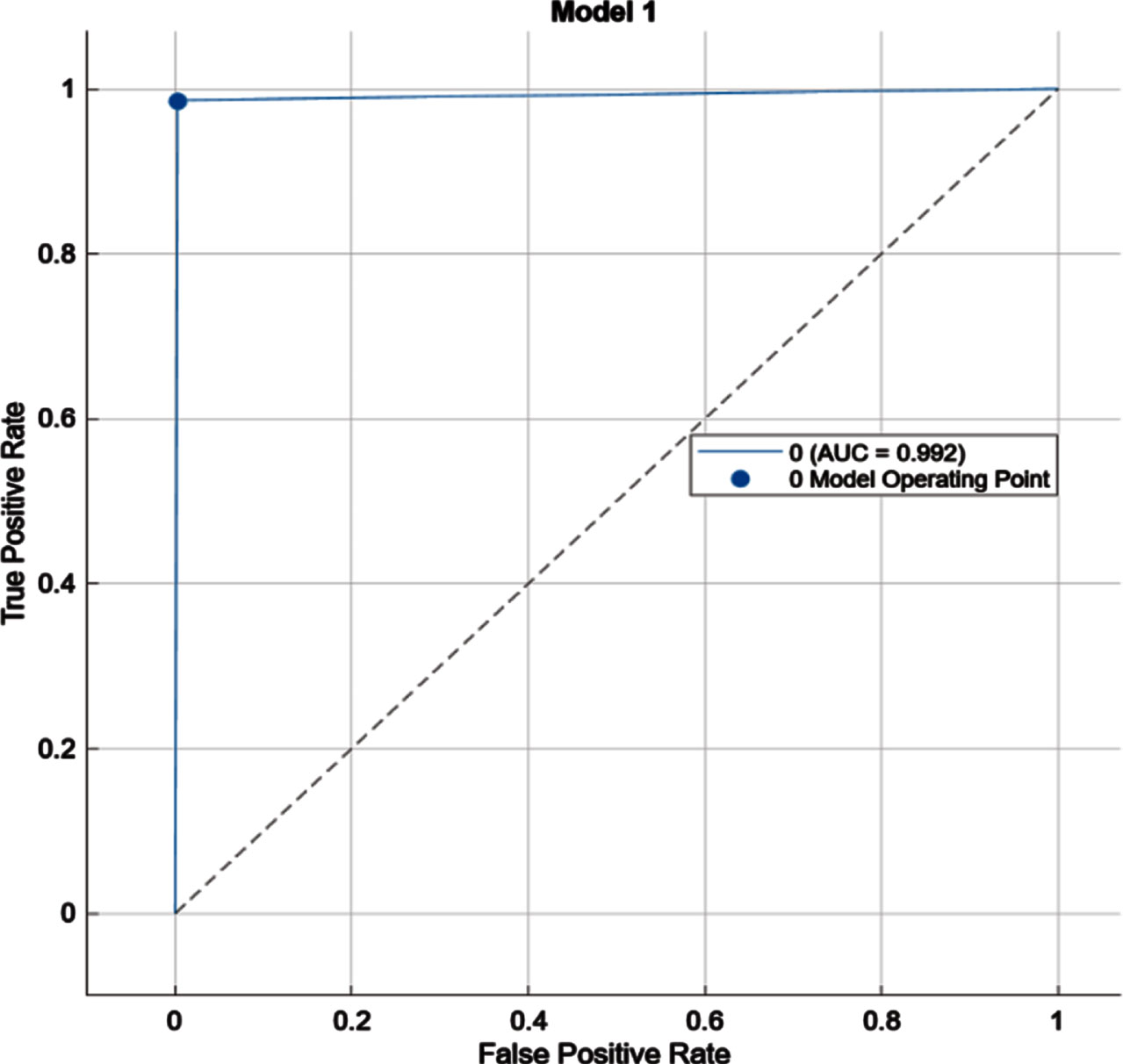
After setting the hyperparameters, the model was trained. The decision tree model achieved 99.4% accuracy and took 10.421 seconds for training. The performance of the model can be studied by Fig. 26 shows the confusion matrix of decision tree classifier. From this confusion matrix we can confirm that model was able to classify defect 3 and defect 4 with a maximum accuracy of 100%. The diagonal elements show the correctly identified data readings for Healthy, Defect1, Defect II, Defect III, Defect IV and Defect V as 98.5%, 98.6%, 99.4%, 100%, 100% and 99.8%. There is least error of 0.2% with error in each classification as 1.5%, 1.4%, 0.6%, 0%, 0% and 0.2% for healthy and respective defects. Figure 27 represents the receiver operating characteristics curve (ROC) which summarizes confusion matrix with different thresholds
Confusion matrix.
ROC curve.
K-Nearest-Neighbours or KNN is simple but efficient non-parametric classification algorithm. KNN (K-Nearest Neighbors) model classifies data points based on neighboring points, it stores all training data in groups and classifies new points based on neighbors. KNN algorithms has high computational cost because computation takes place when classification need to be performed rather than training. When new point is to be classified algorithm calculates distance of neighboring points and find which points are nearest based on this data it classifies [30]. In this study algorithm plots all training data in multidimensional space and when new point is to be classified it calculates Euclidian distance of other points from new point and classifies based on k neighbors, here k is provided as hyperparameter for model. For training the KNN model we need to define k, a number of points to check and distance metric. The Input data for K-NN model is the same labelled data we used for the above two models and we are using K as 2
After setting the hyperparameters, model was trained. The KNN model achieved 97.8% accuracy and took 2.8844 seconds for training. The performance of model can be studied by Fig. 28 and Fig. 29. Figure 28 shows the confusion matrix of KNN classifier from this confusion matrix. Figure 29 represents the receiver operating characteristics curve (ROC) which summarizes confusion matrix with different thresholds. True positive rate and True negative rate can be calculated from the confusion matrix.
Hyperparameters: -
For training KNN the number of neighbors k as 10 and for distance metric we are using Euclidean and distance weight as Equal which is default in MATLAB.
Performance: -
The KNN model took 2.8844 seconds for training and achieved 97.8% accuracy. The performance of model can be studied by Fig. 28 and Fig. 29 which shows the confusion matrix and the ROC curve of KNN classifier from this confusion matrix we can confirm that model was able to classify the diagonal elements as correctly identified or classified color coded as blue and similarly the incorrect sets as peach color. In the healthy set about 639 sets of healthy readings correctly and 12 sets of healthy readings as defect 1 and 5 sets of healthy reading as defect 2. The least amount of reading sets of 583 is identified correctly in the defect 2 and a maximum of 639 sets in healthy readings.

ROC curve.

Confusion Matric.
Random forest is an ensemble-based learning model in which several decision trees are built and output is provided based on the majority tree output. As discussed earlier in decision tree section these algorithms build tree like structure to predict output, in random forest method several decision trees are made with different configurations. For making predictions output of each decision tree in forest is calculated and classification is done based on majority [31]. The output of a random forest is dependent on the number of trees which is the hyperparameter of this model, we are using 30 trees. Ihe input for the random forest is same as of decision tree only difference is of hyperparameters.
ANN
Many studies have shown that Artificial neural networks are best choice for pattern recognition and classification purposes. Multilayer perceptron is type of ANNs which are commonly used for classification purpose and is used in this study also. The purpose of ANN is to find weights and biases for each neuron to minimize error between actual output and model output [2]. A typical MLP consists on one input layer, one or more hidden layers and one output layer. Every neuron takes input vector x and transform it into intermediate vector u based on activation function-
For training model, we first need to define ANN model architecture, our model has 10 input fields which are 10 features selected from MRMR feature selection algorithm and 6 output classes healthy 5 defects we induced. Based on these requirements we need one input layer with 6 neurons, one output layer with 3 neurons and one hidden layer with 10 neurons. Architecture of this ANN model is declared in Fig. 31. For activation function we are using sigmoid function and scaled conjugate gradient algorithm for training this ANN model. For training purpose, we divided data into 70:15:15 ratio for training, testing and validation purpose.

Confusion matrix.
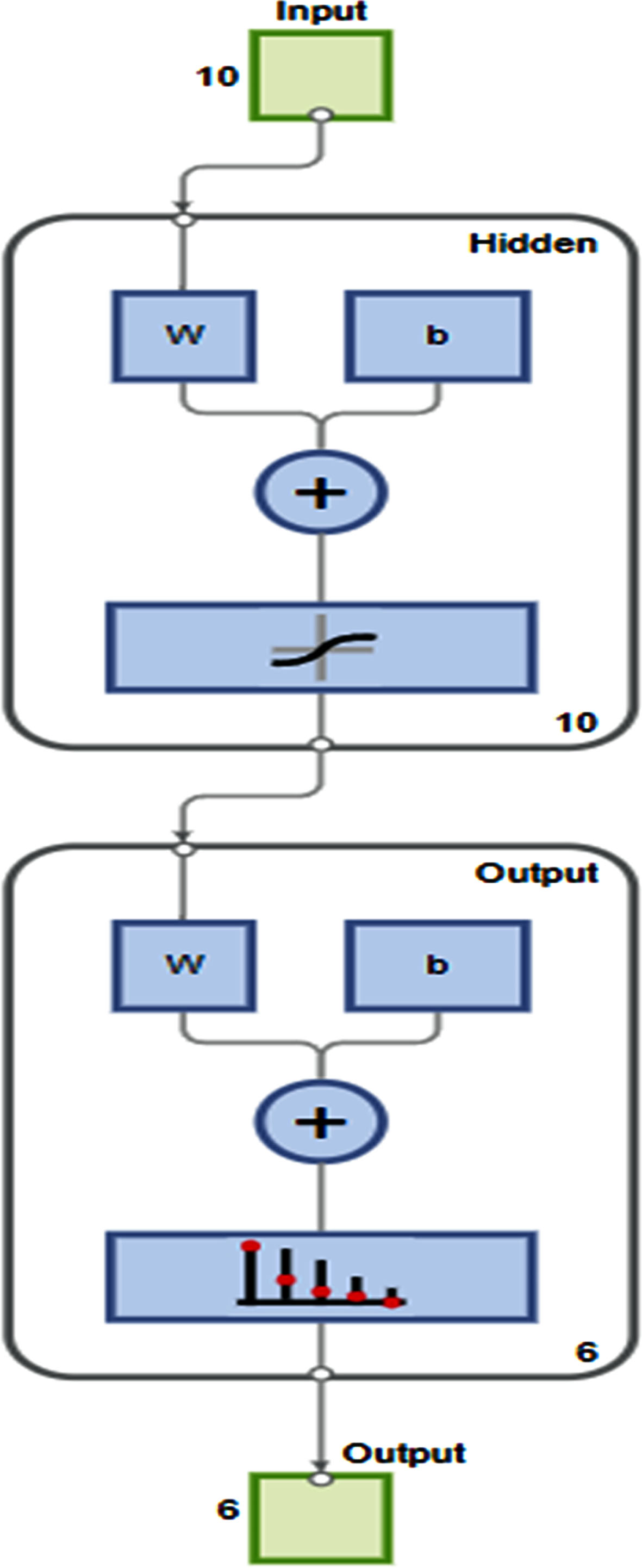
ANN MODEL.
After training model, we got accuracy of about 99.4% and model took around 1.2504 seconds for training. The performance of model is can be studied from Fig. 32, 33, 34 and 35. Figure 32 represents the confusion matrix of the training, testing, and validation dataset. From confusion matrix we can see that model got 99.3% accuracy while training, 99.2% while testing and 98.9% while validation Fig. 34 represents ROC curve for training, testing and validation.
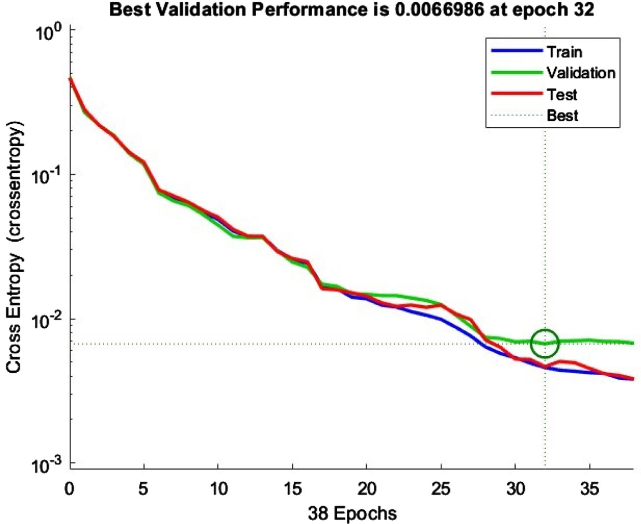
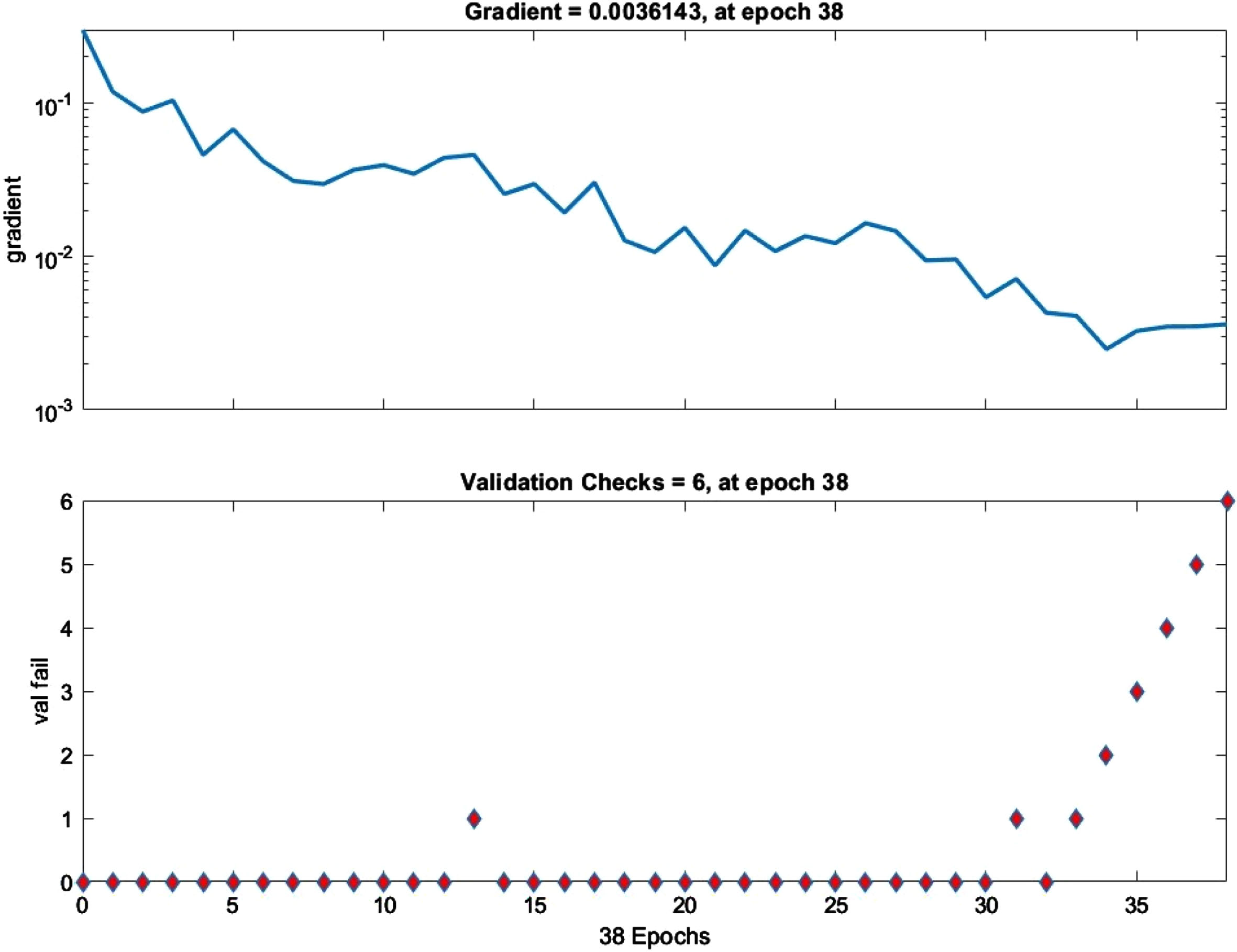
Figure 35 represents the training state, and it can be seen that with increasing epochs gradient is decreasing. The gradient value should be close to zero to minimize the error function at epoch 38 gradient value is 0.0036143, based on this gradient value we can conclude that model is well trained. The validation check occurred at epoch 38 MATLAB set default 6 epochs for validation check therefore, after 38 epochs training was stopped. Figure 33 represents the validation performance of model using cross entropy function. For best performance epoch with lowest validation error is considered which occurred at epoch 32 with validation error of 0.0066986.

Confusion matrix.
ROC curve.

Different ROC curves.
Epochs graphs.
The following paragraphs have been included in the manuscript which is highlighted in yellow colour.
Our study involved training one ANN model and four machine learning models for gearbox fault detection using time and frequency signals to compute statistical parameters.
Nevertheless, validations confirmed the experiment’s credibility, showcasing the adaptability of the neural network and the efficiency of frequency plots in verifying gearbox vibration data. The ANN’s automatic defect identification capability and pattern recognition in statistical features, achieved with a 99.3% accuracy rate, were commendable.
In order to reliably identify gearbox failures using time and frequency signals, our study involved training multiple machine learning models, and Artificial Neural Network (ANN), and extracting ten statistical characteristics for examination. The models shown remarkable potential as each model was able to classify faults with 99.6% accuracy with a computational time of 6.5662 seconds. The decision tree model which has an accuracy of 99.4% and training time of 10.421 seconds is also a computation-intensive model. Though it proved to be computationally demanding, the Decision Tree model trailed in accuracy while the ANN had the highest accuracy of all the models. Hence, the classification rate is good and the results were validated. Thus the various machine learning algorithms were compared.
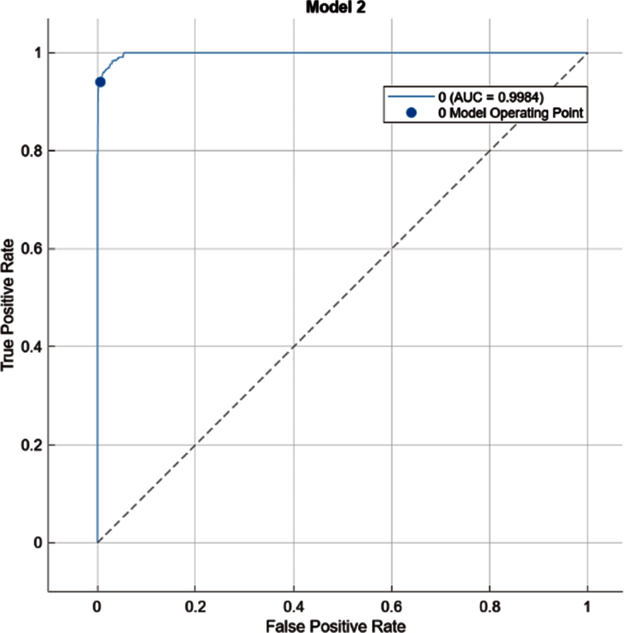
So, for a classification task, we may depend on on an AUC - ROC Curve. We utilise the AUC (Area Under The Curve) ROC (Receiver Operating Characteristics) curve to assess or visualise the performance of the multi-class classification.
The AUC and ROC curve is a performance evaluation for classification issues at various threshold levels. ROC is a probability curve, and AUC reflects the degree or measure of separability. It shows how well the model can discriminate between classes. The higher the AUC, the better the model is in predicting 0 classes as 0 and 1 courses as 1. By correlation, the higher the AUC, the better the model distinguishes between gears with and without the fault.
A pronounced model has an AUC close to 1, indicating that it has a high degree of separability. A bad model has an AUC approaching 0, indicating that it has the weakest measure of separability. In reality, it indicates it is reversing the result. It predicts 0’s as 1’s and 1’s as 0’s. When AUC is less than 0.5, the model has no class separation. Thus the experimental vibration data shows best classification rate using machine learning algorithms.
First, we trained four machine learning models and one ANN model for gear fault detection. The simple workflow for using these models is to take the time domain and frequency signals for the gearbox and calculate 6 statistical parameters and provide these parameters to pre-trained models and then the model will identify the defect. All the models show the potential of identifying gearbox faults with great accuracy. From the outputs of all models, we can find that the ANN has the highest accuracy of 99.6% and a computational time of 6.5662 seconds while SMV has the least accuracy of 96% along with the highest computational time of 21.324 seconds. ANN has easy to adapt and calibrate the vibration data. Also, it has more compatible with various sets of data. The problem with the SMV model is that it requires more computational recourses for prediction because it has to calculate the distance between other points and therefore it takes less time for training. The decision tree model which has an accuracy of 99.4% and training time of 10.421 seconds is also a computation-intensive model.
Reviewing the results, we can say that ANN is the best model for classification because ANN models tend to get more accurate with more data, so if we provide enough data, it can perform even more accurately, on the other hand with SVM models there is a chance of overfitting of data. ANN took about 14.758 seconds less of training time than SVM model. The following Figures. 36 and 37 show the contrast between the training time and accuracy of the models we studied. These training times may change based on computation resources. Based on this research we can conclude that the ANN model is the best approach to detecting gear faults.
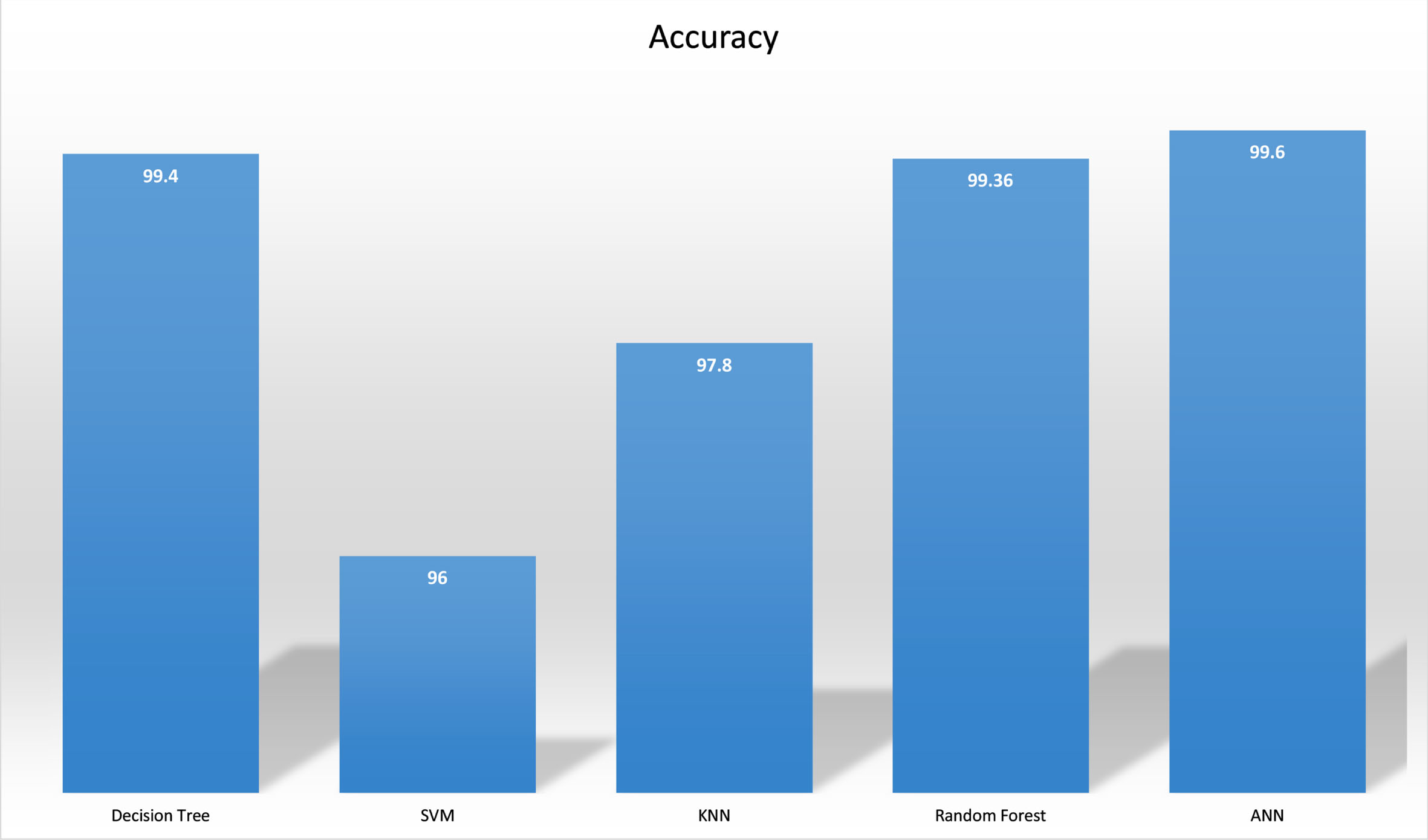
Accuracy comparison.

Training time contrast.