MAO-DBN based membrane fouling prediction

Abstract

Due to the complexity of the factors influencing membrane fouling in membrane bioreactors (MBR), it is difficult to accurately predict membrane fouling. This paper proposes a multi-strategy of integration aquila optimizer deep belief network (MAO-DBN) based membrane fouling prediction method. The method is developed to improve the accuracy and efficiency of membrane fouling prediction. Firstly, partial least squares (PLS) are used to reduce the dimensionality of many membrane fouling factors to improve the algorithm’s generalization ability. Secondly, considering the drawbacks of deep belief network (DBN) such as long training time and easy overfitting, piecewise mapping is introduced in aquila optimizer (AO) to improve the uniformity of population distribution, while adaptive weighting is used to improve the convergence speed and prevent falling into local optimum. Finally, the prediction of membrane fouling is carried out by utilizing membrane fouling data as the research object. The experimental results show that the method proposed in this paper can achieve accurate prediction of membrane fluxes, with an 88.45% reduction in RMSE and 87.53% reduction in MAE compared with the DBN model before improvement. The experimental results show that the model proposed in this paper achieves a prediction accuracy of 98.61%, both higher than other comparative models, which can provide a theoretical basis for membrane fouling prediction in the practical operation of membrane water treatment.

Keywords

Membrane bioreactors (MBR)membrane fouling prediction deep belief network (DBN)aquila optimizer (AO)

1 Introduction

The current serious water environmental problems have driven continuous advancements and innovations in wastewater treatment technology [1]. MBR serves as a crucial tool in wastewater treatment projects, effectively enhancing effluent quality and treatment efficiency. Nonetheless, the formation of membrane fouling significantly affects the operational stability and economic viability of the system, thereby restricting the widespread application of MBR [2 –4]. Consequently, it becomes imperative to forecast and prevent membrane fouling [5 –7].

Machine learning can be used to predict membrane pollution by mining hidden patterns in large amounts of historical data. Among them, artificial neural network (ANN) is a commonly used machine learning model with the advantages of fewer parameters, good prediction performance and strong generalization ability, so it is widely used in the field of wastewater treatment [8 –10]. In order to construct predictive models for the transmembrane pressure (TMP) at various stages of the MBR production cycle, data-driven machine learning techniques such as random forest (RF), ANN and long short-term memory (LSTM) are employed in the literature [11]. The proposed model has better prediction accuracy than the ANN or LSTM model. Literature [12] describes the effects of concurrent upward and downward aeration on both membrane fouling and process performance in submerged membrane bioreactors. To simulate TMP and membrane permeability (Perm), the authors utilized multilayer perceptron and radial basis function artificial neural networks (MLPANN and RBFANN). To optimize the models, genetic algorithms (GA) were employed to adjust the weights and thresholds. The results demonstrate that the optimized model exhibits high accuracy in predicting outcomes. Literature [13] proposed the use of back propagation neural networks (BP) for the simulation and prediction of MBR membrane fluxes, and combined tent mapping and sparrow search algorithm (SSA) to improve its global search capability and fast convergence ability. Based on the results, the Tent-SSA-BP prediction model outperforms the traditional BP neural network prediction model, improving the shortcomings of local extremes and poor generalization ability. However, in a complex problem such as membrane fouling prediction, which usually involves multiple influencing factors and complex nonlinear relationships, simple machine learning models have drawbacks in membrane fouling prediction such as limited expressive power, underfitting or overfitting, and sensitivity to noise and outliers [14].

To address these problems, deep learning neural network (DLNN) has been widely used in membrane fouling prediction research to compensate for the shortcomings of simple ANNs and ANNs combined with optimization algorithms, with their excellent ability to mine the deep nature of data, flexible representation of highly variable non-linear relationships [15, 16]. In literature [17], a novel hybrid metaheuristic algorithm named adaptive particle swarm optimization whale optimization algorithm (APSOWOA) was proposed for optimizing hyperparameters in convolutional neural networks. The fitness value of the APSO-WOA optimization algorithm is defined as the cross-entropy loss function of the validation set during CNN model training. The results demonstrate that the APSOWOA-CNN model exhibits higher predictive accuracy and reliability. However, convolutional neural networks are vulnerable to adversarial sample attacks when dealing with two-dimensional data, which can lead to misjudgment of the prediction results of convolutional neural networks through minor perturbation of the input data. Deep neural network (DNN) has higher accuracy and precision in prediction compared to traditional machine learning algorithms due to its deep structure and a large number of tunable parameters. Literature [18] combined the DNN model with stochastic standard deviation sampling (RSDS) to develop an RSDS-DNN model that simulates the complex anaerobic digestion process in biochemical wastewater and predicts the production of unbound hydrogen sulfide, thereby improving methane production by mitigating the inhibition of unbound hydrogen sulfide. inhibition to improve methane production. However, DNNs typically require large amounts of labeled data to train and tune the model, which degrades the performance of DNNs with fewer data or inaccurate labeling, and DNNs are highly flexible and expressive and may overfit on the training set, resulting in degraded performance on the test set. DBN can train the deep structure by pre-training and fine-tuning layer by layer, thus avoiding the problem of gradient disappearance or gradient explosion encountered in deep network training, and training the model by unsupervised learning without the need for labeled data, thus having an advantage when the amount of data is large but labeling is difficult. Literature [19] proposed a prediction model based on a genetic deep trust network algorithm. GA is used to reduce the dimensionality of the input variables, simplify the network structure and overcome the difficulties of dynamic features of process data in monitoring. Compared to DBN and BP neural networks, GA-DBN effectively achieves better prediction accuracy than other tested models in complex wastewater treatment processes. However, the model structure of DBN is more complex and requires significant computational resources and time for training and testing, especially on large-scale datasets. During the training phase, layer-by-layer pre-training and fine-tuning are required, resulting in longer training times and high computational resources. This makes DBNs expensive to train and debug, and difficult to apply in some resource-constrained situations. The performance of DBN is dependent on the quality and quantity of data, and too little or low-quality data can affect the performance of the model. If the data is noisy or unbalanced, the performance of the DBN will also be affected.

To compensate for the above disadvantages of deep learning neural networks, both traditional parameter optimization methods and population parameter optimization algorithms are widely used. However, they have different advantages in solving complex problems. Traditional parameter optimization methods such as grid search, stochastic search, and gradient descent provide simple and intuitive optimization frameworks. In contrast, population parameter optimization algorithms such as GA and PSO possess stronger global search capability and adaptivity by simulating population behavior and interaction. For complex problems such as membrane fouling prediction, traditional parameter optimization methods have some limitations. In contrast, population intelligent optimization algorithms can better cope with multiple influencing factors and complex nonlinear relationships in membrane fouling prediction through the advantages of global search capability, adaptivity, robustness, and parallelism. The aquila optimizer (AO) is a novel heuristic optimization algorithm that employs efficient search strategies, such as local and global search, as well as escaping from local optima, to achieve fast and effective search. This new type of heuristic optimization algorithm, as described in literature [20], combines various efficient search strategies to quickly find the optimal solution. The AO algorithm has strong robustness and can handle a variety of complex non-linear optimization problems. The AO algorithm is independent of the initial point and can search for the same global optimal solution at different initial points. Literature [21] introduced the aquila optimizer algorithm-based echo state network (AO-ESN) for predicting the grounding resistance of offshore wind turbines. The three networks, BP, ESN and AO-ESN, are compared separately, and the proposed method in the paper has the highest accuracy compared with other models, which reflects the superiority of the method. In literature [22], a novel AO-CNN model is introduced to predict spindle thermal errors in CNC machine tools. This model effectively addresses the issue of spindle thermal errors adversely affecting machining accuracy. By leveraging the optimal solving capability of AO and the self-learning and self-adaptive capabilities of CNN, the proposed AO-CNN model provides accurate predictions of spindle thermal errors in CNC machine tools. The results show that the thermal error modeling using AO-CNN improves the prediction accuracy by 15% compared to the CNN model. However, the AO algorithm also has shortcomings. Firstly, the search results are strongly influenced by the initial population. If the initial point is not selected properly, it may fall into a local optimum solution and fail to jump out. Secondly, during the search process, the aquila optimization algorithm may suffer from a premature convergence problem, the search process stops too early, resulting in the inability to find the global optimal solution.

Based on this, shallow machine learning is widely used in current research on membrane fouling prediction, it has limitations in capturing the complexity of contamination mechanisms and handling large-scale data. The emergence of DLNN methods provides new opportunities for advancing membrane fouling prediction. In this paper, we first employ the PLS method to select auxiliary variables, addressing the challenge of complex factors influencing membrane fouling. Next, we introduce piecewise chaotic mapping into the AO algorithm for population initialization, enhancing population diversity and preventing local optima. To expedite the AO algorithm’s search for the optimal solution, we introduce adaptive weights and develop the MAO algorithm. Finally, we integrate MAO with DBN networks to construct a soft measurement model for MAO-DBN membrane flux. The reliability and stability of the model are validated using simulation data from the Seong Hoon Yoon spreadsheet model. Additionally, to account for the uncertainty in membrane module operation under actual conditions, we introduce Gaussian white noise to further evaluate the model’s robustness.

2 Theory related to DBN

This section introduces the network structure of RBM, the DBN network structure, and the training process. Their network structure and training process provide an effective unsupervised learning method for deep learning, which provides a powerful tool for solving such complex tasks as membrane fouling and processing large-scale data.

2.1 RBM network structure

Hinton proposed the DBN in 2006 [23], which is a generative model based on deep learning techniques. It consists of several restricted boltzmann machines (RBMs), where the RBM has only two layers of neurons [7].

The RBM structure is shown in Fig. 1, where the visual layer contains m nodes, the implicit layer contains n nodes, and the connection weights are denoted as. The individual connection weights in the DBN network can be further optimized using multilayer unsupervised learning and supervised fine-tuning [24]. The weights of the whole DBN can be obtained by fine-tuning them sequentially from the top output layer to the bottom input layer.

Fig. 1

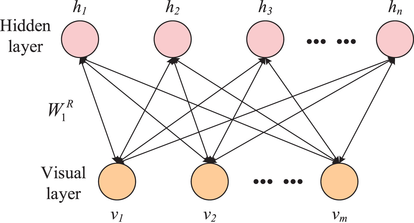
RBM model structure.

2.2 DBN network architecture

DBN consists of several RBMs stacked sequentially, where the output of each RBM is used as training input for the next RBM. As a generative model, the learning process of a DBN can be divided into two stages. The first stage is layer-by-layer unsupervised pre-training, through which the initial weights of the entire network are determined. The second stage is supervised fine-tuning, which uses the initial weights that have been determined to optimize [25]. The structure of the DBN is shown in Fig. 2.

Fig. 2

DBN model structure.

In Fig. 2, y_sis the desired output of the network and w = (wout, w_l, w_l-1, ⋯ , w₂, w₁) is the connection weights of the network, which can be obtained by supervised fine-tuning of the initial weights determined by unsupervised learning at $w^{R} = (w_{l}^{R}, w_{l - 1}^{R}, w_{l - 1,} \dots, w_{1}^{R})$ . The goal of unsupervised pre-training of DBNs is to determine the initial weights of the entire network by training each RBM layer by layer. It has been shown that using this unsupervised algorithm to initialize the DBN weights usually gives better training results than randomly initializing the weights, and the purpose of supervised learning is to fine-tune the weights obtained from unsupervised learning [26].

2.3 DBN training process

Hinton employs an unsupervised training technique to obtain the parameters that determine the initial weights of the network. In the RBM model, the visible and hidden layers are represented as v and h, respectively. By considering the model’s parameters, the joint probability distribution can be defined using an energy function that captures the relationship between the visible and hidden layers. Consequently, the weights obtained through this method ensure enhanced network performance.

In the RBM model, the weights between each cell in different layers and the deviations on individual cells are defined as probability distributions utilizing an energy function. For bernoulli-bernoulli type RBMs, the energy function is given as. $E (v, h | θ) = - \sum_{i = 1}^{m} \sum_{j = 1}^{n} v_{i} w_{ij}^{R} h_{j} - \sum_{i = 1}^{m} a_{i} v_{i} - \sum_{j = 1}^{n} b_{j} h_{j}$ (1) whereθ = { w^R, a, b } is the requested parameter, $w_{ij}^{R}$ is the connection weight of the RBM, a_i and b_j are the biases of the visible and hidden layer cells, respectively. When the parameters are determined, the joint probability distribution of (v, h) can be obtained. $P (v, h | θ) = \frac{1}{Z} e^{- E (v, h; θ)}$ (2) where Z = ∑_v,he^-E(v,h;θ) is the normalization factor and the marginal distribution of the model concerning: $P (v | θ) = \frac{1}{Z} \sum_{v, h} e^{- E (v, h; θ)}$ (3)

The probability of activation of neurons in the visual and implicit layers as: $P (h_{j} = 1 | v, θ) = σ (b_{j} + \sum_{i = 1}^{m} v_{i} w_{ij}^{R})$ (4) $P (v_{i} = 1 | v, θ) = σ (b_{j} + \sum_{j = 1}^{n} w_{ij}^{R} h_{j})$ (5) where σ is the activation function. The RBM parameters were trained by gradient descent based on the maximum likelihood estimation of the training as: $θ^{*} = θ + ξ \frac{\partial ln p (v)}{\partial θ}$ (6) $\begin{matrix} \frac{\partial ln p (v)}{\partial θ} = \sum t = 1 N [{(\frac{\partial (- E (v^{(t)}, h | θ))}{\partial θ})}_{p (h | v, θ)}] \\ - \sum_{t = 1}^{N} [{(\frac{\partial (- E (v, h | θ))}{\partial θ})}_{p (h | v, θ)}] \end{matrix}$ (7) where ξ denotes the learning rate and N denotes the number of samples. Then the update rule for the RBM parameter θ is: ${\begin{matrix} \frac{\partial ln p (v)}{\partial w_{i, j}} = ξ ({〈 v_{i} h_{j} 〉}_{data} - {〈 v_{i} h_{j} 〉}_{recon}) \\ \frac{\partial ln p (v)}{\partial α_{i}} = ξ ({〈 v_{i} 〉}_{data} - {〈 v_{i} 〉}_{recon}) \\ \frac{\partial ln p (v)}{\partial b_{j}} = ξ ({〈 h_{j} 〉}_{data} - {〈 h_{j} 〉}_{recon}) \end{matrix}$ (8) where 〈 · 〉 _data represents the expectation of the training sample and 〈 · 〉 _recon represents the expectation of the reconstructed model. From there, the initial weights and biases are determined.

At this point, the training of one layer of RBM is completed. Similarly, the weights and offsets of the parameters of the first layer of RBM₁ are used as the initial weights and offsets of the visible layer of the next layer of RBM₂ through the hidden layer h₁ of RBM₁ in the DBN until the iteration is completed.

3 Aquila optimization algorithm

This section focuses on the development of the MAO algorithm. Firstly, the optimization search process of the AO algorithm is introduced. Then, piecewise chaotic mapping is introduced in the algorithm to initialize the population. In order for the AO algorithm to find the optimal solution faster, adaptive weights are further introduced to construct the MAO algorithm. Finally, comparative experiments with other optimization algorithms are conducted using test functions to illustrate the advantages of the MAO algorithm.

3.1 Basic aquila optimization

(1) Initialization

The aquila optimizer is based on a population intelligence algorithm, which, when building a mathematical model, requires first randomly initializing the population’s position matrix X: $X = [\begin{matrix} x_{1, 1} \dots x_{1, j} x_{1, Dim - 1} x_{1, Dim} \\ x_{2, 1} \dots x_{2, j} \dots x_{2, Dim} \\ \dots \dots x_{i, j} \dots \dots \\ ⋮ ⋮ ⋮ ⋮ ⋮ \\ x_{N - 1, 1} \dots x_{N - 1, j} \dots x_{N - 1, Dim} \\ x_{N, 1} \dots x_{N, j} x_{N, Dim - 1} x_{N, Dim} \end{matrix}]$ (9) where X denotes a set of current candidate solutions that are randomly generated using equation (9), X_i denotes the decision value (position) of the ith solution, N denotes the total number of candidate solutions (overall), and Dim denotes the dimensionality of the problem. $\begin{matrix} X_{ij} = rand \times ({UB}_{j} - {LB}_{j}) + {LB}_{j}, \\ i = 1, 2, \dots, N j = 1, 2, \dots, Dim \end{matrix}$ (10) where rand is a random number, LB_j denotes the j-th lower bound of the given problem, and UB_j denotes the j-th upper bound of the given problem.

(2) Expanded exploration phase

In the initial phase, the Aquila optimizer conducts an expanded exploration by flying at a high altitude to identify the prey area. This allows the searcher to explore the search space and locate the region where the prey is located. This behavior is mathematically represented by Equation (11): $\begin{matrix} X_{1} (t + 1) = X_{best} (t) \times (1 - \frac{t}{T}) \\ + (X_{M} (t) - X_{best} (t) * rand) \end{matrix}$ (11)

X_best (t) is the optimal solution before the t-th iteration, representing the approximate position of the prey. 1 - t/T Used to control the extended search by the number of iterations. X_M (t) denotes the mean value of the position of the current solution connected at the t-th iteration. rand is a random value between 0 and 1. t and T denote the current and maximum number of iterations, respectively. X_M (t) the formula for the calculation is as: $X_{M} (t) = \frac{1}{N} \sum_{i = 1}^{N} X_{i} (t), \forall j = 1, 2, \dots, Dim$ (12)

(3) Narrow the search phrase

In the second phase, the Aquila optimizer uses contour flight, a method of hovering above the prey before landing and attacking. The AO narrows its exploration to focus on a specific area of the prey in preparation for the attack. The mathematical model of this behavior is shown in Equation (13): $\begin{matrix} X_{2} (t + 1) = X_{best} (t) \times Levy (D) \\ + X_{R} (t) + (y - x) * rand \end{matrix}$ (13) where D represents the dimensional space, and Levy(D) is the Levy flight distribution function, calculated from Equation (14). X_R (t) is the random solution taken in the range [1, N] at the R-th iteration. $Levy (D) = s \times \frac{u \times σ}{{| v |}^{\frac{1}{β}}}$ (14)

where s is a constant value fixed to 0.01, u, and v are random numbers between 0 and 1. σ is calculated as follows: $σ = {(\frac{Γ (1 + β) \times sin (\frac{π β}{2})}{Γ (\frac{1 + β}{2}) \times β \times 2 (\frac{β - 1}{2})})}^{\frac{1}{β}}$ (15) where β is a constant value fixed to 1.5. In Equation (15), y and x are used to represent the shape of the spiral in the search, which is calculated as follows: $y = r \times cos (θ), x = r \times sin (θ)$ (16)

Of which $r = r_{1} + U \times D_{1}, θ = - ω \times D_{1} + \frac{3 π}{2}$ (17) where r₁ takes a value between 1 and 20 for fixed the number of search cycles, and U is a small value fixed to 0.00565. D1 is integer numbers from 1 to the length of the search space (Dim), and ω is a small value fixed to 0.005.

(4) Expansion of the development phase

In the third phase, the Aquila optimizer accurately designates the prey area and prepares to land and attack. It descends vertically and initiates an initial attack to observe the prey’s reaction. This approach is known as a low-level slow descent attack, where the AO uses a specific region of the target to approach and launch the attack. Equation (18) demonstrates this behavior mathematically: $\begin{matrix} X_{3} (t + 1) = (X_{best} (t) - X_{M} (t)) \times α - rand \\ + ((UB - LB) \times rand + LB) \times δ \end{matrix}$ (18) where: the lower and upper bounds of the problem are denoted by LB and UB, respectively, α and δ are the exploitation adjustment parameters fixed in this algorithm to a small value 0.1.

(5) Narrowing the development

In the fourth stage, the AO approaches the prey and launches an attack on land using random movements. This method, known as “walk and catch the prey,” involves attacking the prey in its last known position. The mathematical model of this behavior is shown in Equation (19): $\begin{matrix} X_{4} (t + 1) = QF (t) \times X_{best} (t) - (G_{1} \times X (t) \times rand) \\ - G_{2} \times Levy (D) + rand \times G_{1} \end{matrix}$ (19) where: QF(t) denotes the prime function used to equilibrate the search strategy, G₁ denotes the various movements of the aquila tracking the fleeing prey, and the value of G₂ decreases from 2 to 0. This indicates the gradient of the aquila’s flight from the first position to the last position during the tracking of the prey, denoted as $QF (t) = t^{\frac{2 \times rand - 1}{(1 - T)^{2}}}$ (20) $G_{1} = 2 \times rand - 1$ (21) $G_{2} = 2 \times (1 - \frac{t}{T})$ (22)

3.2 Improved aquila optimization algorithm

3.2.1 Piecewise chaotic mapping population initialization

To address the issue of population initialization and prevent the algorithm from getting trapped in local optima, a chaotic sequence generated by a chaotic mapping can be employed [27]. In AO algorithm, the initial position information is randomly generated, resulting in insufficient population diversity. Therefore, during the extended exploration phase, piecewise chaotic mappings are introduced to generate well-initialized populations and enhance population diversity. This approach also mitigates the problem of uneven population distribution that may occur during the optimization process, thereby accelerating convergence and improving convergence accuracy. The mathematical expression of the piecewise chaotic mapping is: $x (t + 1) = {\begin{matrix} \frac{x (t)}{p} 1 pt, 0 ⩽ x (t) < p \\ \frac{x (t) - p}{0.5 - p}, p ⩽ x (t) < 0.5 \\ \frac{1 - p - x (t)}{0.5 - p}, 0.5 ⩽ x (t) < 1 - p \\ \frac{1 - x (t)}{p}, 1 - p ⩽ x (t) < 1 \end{matrix}$ (23) where p is a control parameter and p = 0.4, x(t) takes values in the range [0,1].

Figure 3 and 4 compare the effect of the algorithm on population initialization after logistic chaos mapping and piecewise chaos mapping. Figure 3(a) shows the histogram generated by the logistic chaos mapping, which exhibits an irregular shape, due to the high randomness generated by the chaos mapping, resulting in an uneven distribution of data in the histogram. In contrast, Fig. 4(a) shows the histogram generated by the piecewise chaos mapping, which exhibits a relatively stable shape, indicating that the piecewise chaos mapping can result in a more uniform distribution of data. Figure 3(b) and Fig. 4(b) show the population distributions after using the logistic mapping and the piecewise mapping respectively. It can be seen that after initialization using the piecewise mapping, the population distribution is more dispersed and there are fewer individuals on the boundary and overlapping individuals. In the initialization stage, a larger distribution breadth can ensure the diversity of the population, while reducing the attraction of local optimal solutions. Therefore, this paper chooses to use piecewise mapping as the method of population initialization.

Fig. 3

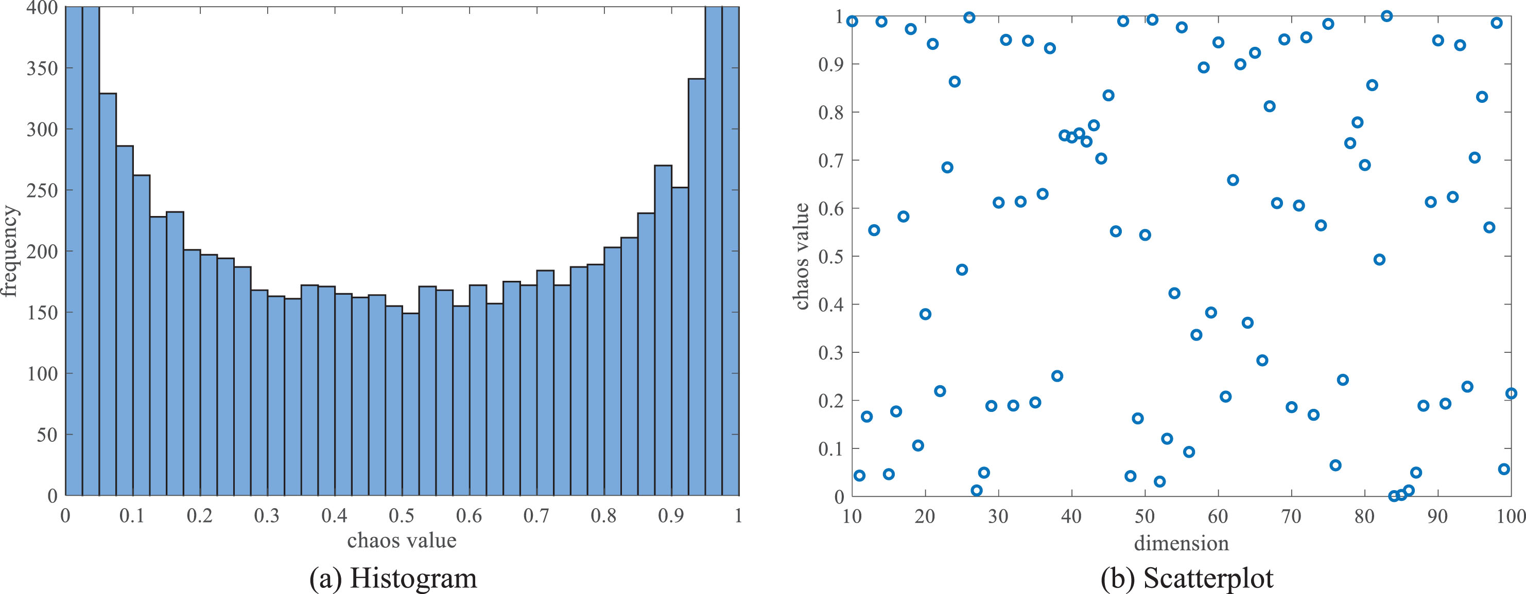
Logistic chaotic mapping.

Fig. 4

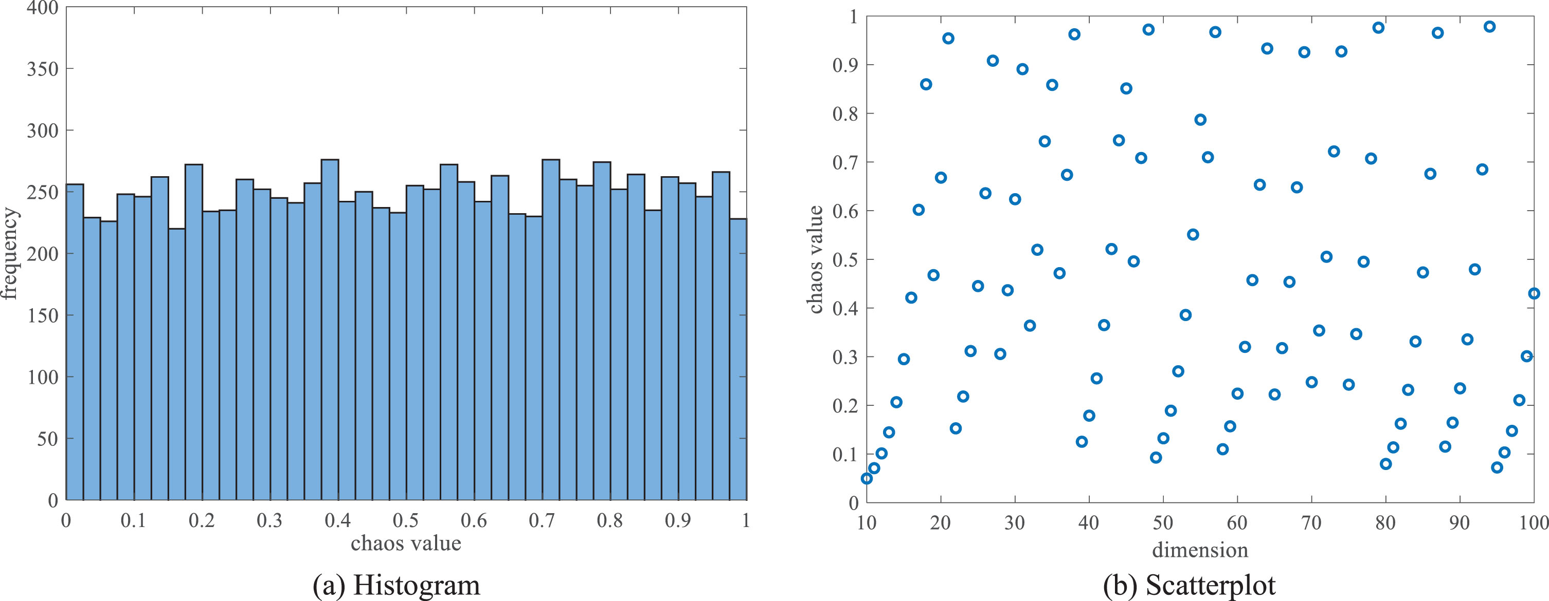
Piecewise chaotic mapping.

3.2.2 Adaptive weights

In the aquila optimization algorithm, weights are commonly used to adjust the exploration and exploitation strategies during the search process, aiming to enhance the algorithm’s ability to search for the optimal solution in the solution space. In the aquila optimization algorithm, weights are primarily applied in the following two ways:

The flight strategy of the aquilas includes exploration and exploitation strategies, and the weights are adjusted to balance the ratio between exploration and exploitation.

movement step size of the aquilas can also be influenced by adjusting weights, which impacts the search range and speed, ultimately aiding in finding the optimal solution.

The weights in the AO algorithm play a crucial role in balancing global search and local exploration. Fixed weights can lead to being trapped in local optima, hindering the discovery of the global optimum. In complex problems like membrane fouling, fixed weights may not effectively utilize available data, resulting in suboptimal performance. Consequently, adapting the algorithm to different optimization problems can pose significant challenges.

To address the issue of balancing exploration and exploitation in the AO algorithm, an adaptive inertia weight ω is proposed. This weight starts with a larger value to enable swift global exploration at the beginning of an iteration and gradually decreases towards the end to enhance local exploration. The calculation of the adaptive inertia weights is performed as follows: $ω = {exp}^{(\frac{- 2 t}{T - t})}$ (24) where, T represents the maximum number of iterations, and the improved formula is given as follows: $x_{best}^{'} = x_{best} \times (1 - {exp}^{(\frac{- 2 t}{T - t})})$ (25)

Figure 5 shows that the total number of iterations is 200. In the early iterations, the rate of non-linear change is faster and the weights are larger, which is beneficial to the global exploration ability. In the late iterations, the rate of non-linear change is slower and the weights are smaller, which is beneficial to the local exploration ability.

Fig. 5

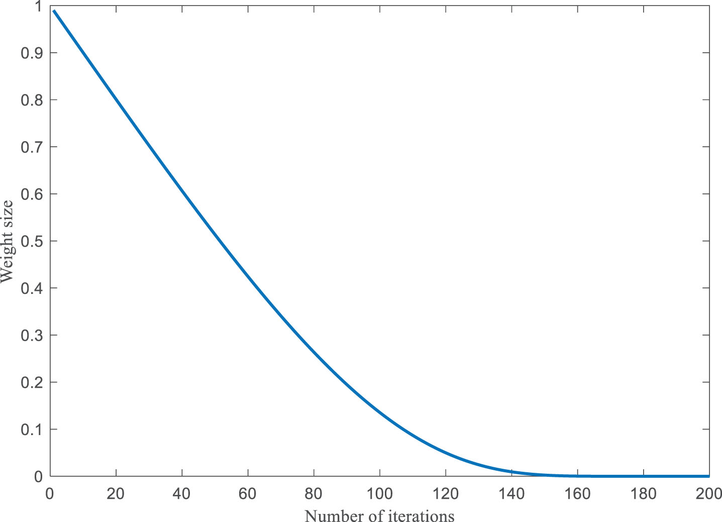
Adaptive weight change curve.

3.2.3 Improved algorithm performance

This section focuses on comparing the effectiveness of MAO through comparative experiments with various algorithms. Table 1 provides a list of the six benchmarking functions. For a more intuitive comparison, we used the Particle Swarm Optimization algorithm (PSO), Whale Optimization algorithm (WOA), Aquila Optimization algorithm (AO), and Multi-Strategy Integrated Particle Swarm Optimization algorithm (MPSO) as reference algorithms, as shown in Fig. 6. Each algorithm was configured with a maximum of 200 iterations an d 30 population size. The tests were conducted using the six benchmark functions described in Table 1, which consist of single-peak functions (F1, F2, and F3) and multi-peak. The single-peak test function primarily assesses the convergence speed and accuracy of the algorithm, whereas the multi-peak test function primarily evaluates the global search capability and robustness of the algorithm.

Table 1
Test functions

Test functions Range of values Dimension Theoretical minimum

$F_{1} (x) = \sum_{i = 1}^{n} x_{i}^{2}$ _[–100,100] ₃₀ ₀

$F_{2} (x) = \sum_{i = 1}^{n - 1} [100 (x_{i + 1} - x_{i}^{2})^{2} + (x_{i} - 1)^{2}]$ _[–30,30] ₃₀ ₀

$F_{3} (x) = \sum_{i = 1}^{n} {([x_{i} + 0.5])}^{2}$ _[–100,100] ₃₀ ₀

$F_{4} (x) = - 20 exp (- 0.2 \sqrt{\frac{1}{n} \sum_{i = 1}^{n} x_{i}^{2}}) - exp (\frac{1}{n} \sum_{i = 1}^{n} cos (2 π x_{i})) + 20 + e$ _[–32,32] ₃₀ ₀

$F_{5} (x) = \frac{1}{4000} \sum_{i = 1}^{n} x_{i}^{2} - \prod_{i = 1}^{n} cos (\frac{x_{i}}{\sqrt{i}}) + 1$ _[–600,600] ₃₀ ₀

$F_{6} (x) = \sum_{i = 1}^{11} {[a_{i} - \frac{x_{1} (b_{i}^{2} + b_{1} x_{2})}{b_{i}^{2} + b_{1} x_{3} + x_{4}}]}^{2}$ _[–5,5] ₄ _0.1484

Test functions	Range of values	Dimension	Theoretical minimum
$F_{1} (x) = \sum_{i = 1}^{n} x_{i}^{2}$	_[–100,100]	₃₀	₀
$F_{2} (x) = \sum_{i = 1}^{n - 1} [100 (x_{i + 1} - x_{i}^{2})^{2} + (x_{i} - 1)^{2}]$	_[–30,30]	₃₀	₀
$F_{3} (x) = \sum_{i = 1}^{n} {([x_{i} + 0.5])}^{2}$	_[–100,100]	₃₀	₀
$F_{4} (x) = - 20 exp (- 0.2 \sqrt{\frac{1}{n} \sum_{i = 1}^{n} x_{i}^{2}}) - exp (\frac{1}{n} \sum_{i = 1}^{n} cos (2 π x_{i})) + 20 + e$	_[–32,32]	₃₀	₀
$F_{5} (x) = \frac{1}{4000} \sum_{i = 1}^{n} x_{i}^{2} - \prod_{i = 1}^{n} cos (\frac{x_{i}}{\sqrt{i}}) + 1$	_[–600,600]	₃₀	₀
$F_{6} (x) = \sum_{i = 1}^{11} {[a_{i} - \frac{x_{1} (b_{i}^{2} + b_{1} x_{2})}{b_{i}^{2} + b_{1} x_{3} + x_{4}}]}^{2}$	_[–5,5]	₄	_0.1484

Fig. 6

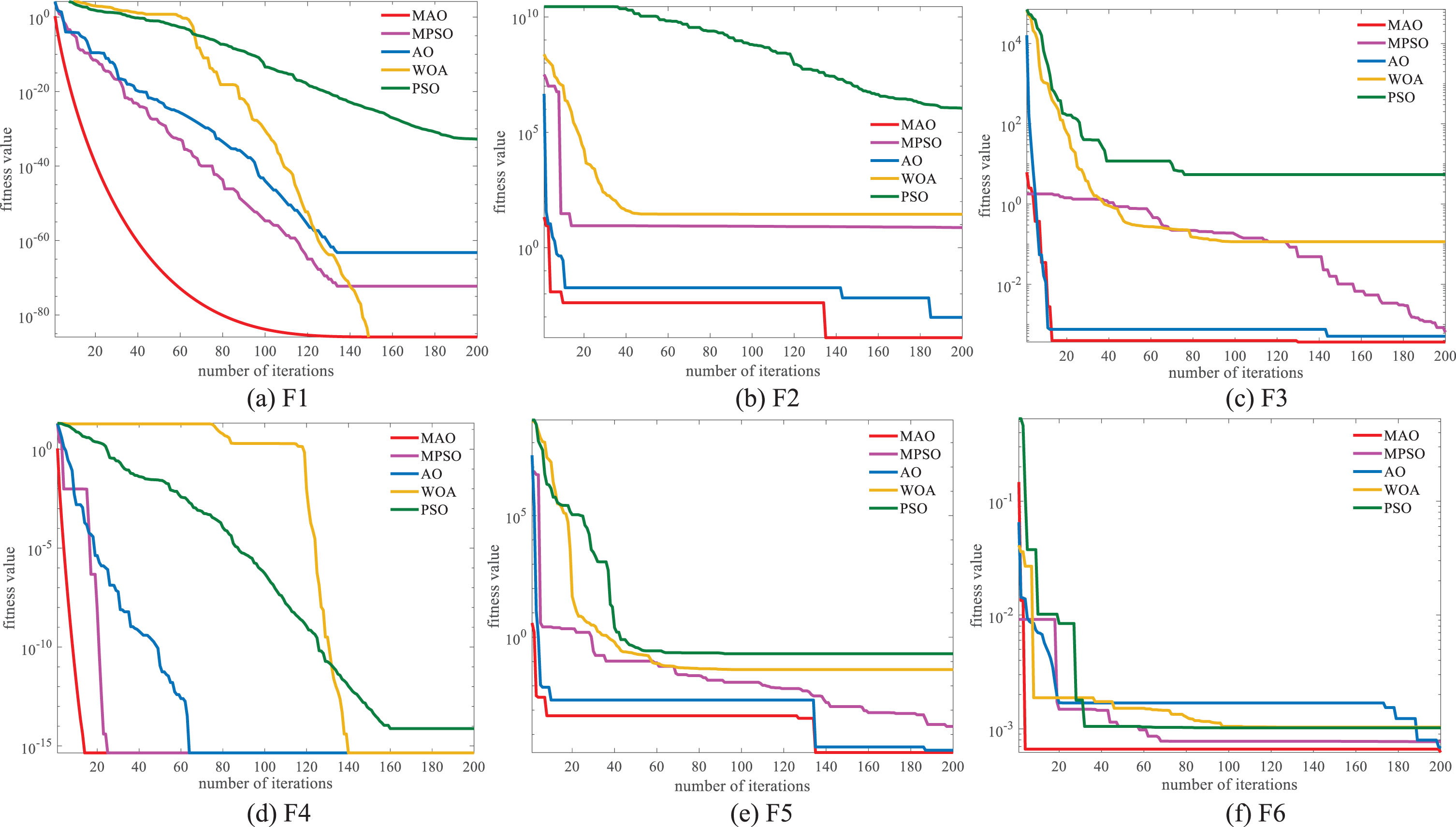
Iterative convergence curves for different test functions.

From Fig. 6, it can be observed that the MAO algorithm exhibits a significant improvement in convergence speed in the early stages compared to other intelligent algorithms for the six benchmark functions. The exploration period of the algorithm is greatly reduced, leading to enhanced optimization search performance by efficiently exploring the search space and improving global search capabilities. Additionally, the algorithm takes optimization accuracy into account, enabling it to reach the optimal solution more quickly.

Furthermore, the comparative analysis between MPSO and PSO also reveals that MPSO demonstrates improvements in both convergence speed and accuracy. For the function F3, the MAO algorithm does not exhibit a significant improvement in convergence speed compared to AO, but it achieves enhanced convergence accuracy. Similarly, for the function F4, MAO does not show significant improvements in convergence accuracy compared to AO and WOA, but it improves convergence speed. Consequently, it can be concluded that MAO exhibits faster, more stable, and more accurate convergence in both single-peak and multi-peak tests.

4 Membrane fouling prediction model

This section outlines the modeling process for predicting membrane fouling. The key factors that contribute to membrane fouling are first described. These factors are then downscaled using the PLS method. Finally, the construction of the MAO-DBN predictive model based on membrane fouling is presented.

4.1 The factors influencing membrane fouling

Membrane fouling is caused by a combination of factors. These factors include membrane materials, reactor operating conditions and sludge mix characteristics. The nature of the membrane material includes material, hydrophobicity and roughness, while the operating conditions of the MBR system, such as influent water quality, operating temperature, sludge retention time (SRT), hydraulic retention time (HRT), operating pressure and trans-membrane pressure (TMP), can also affect membrane fouling. In addition, characteristics such as total suspended solids (TSS), mixed liquor suspended solids (MLSS), particle size distribution (PSD), extracellular polymeric substances (EPS) and soluble microbial products (SMP) in the sludge mix are also important factors affecting membrane fouling. In addition to flow rate, air-to-water ratio, pressure in the produced water, viscosity, biochemical oxygen demand (BOD), chemical oxygen demand (COD), the wastewater treatment process emits several variables, such as pH and oxidation-reduction potential (ORP), which can also have an impact on membrane fluxes [28]. Therefore, the interactions between membrane fouling factors and their effects on membrane fouling need to be fully investigated when constructing a membrane fouling prediction model.

4.2 Variable selection

PLS is a commonly used data dimensionality reduction method that reduces high-dimensional datasets to low-dimensional and retains as much information as possible about the original data [29]. One of the advantages of PLS is its ability to address multicollinearity issues and effectively filter auxiliary variables that exhibit the strongest correlation with membrane fluxes.

Let X represent the independent variable and Y the dependent variable. In PLS, components ti and uj are extracted from X and Y, respectively. The algorithm performs iterative calculations for each dimension, utilizing information from both variables. In each iteration, ti and uj are continuously adjusted for the subsequent round of component extraction based on the residual information of X and Y. The algorithm repeats this process until the absolute values of the residual matrices’ elements meet the required accuracy, at which point it terminates. Throughout the iterations, ti and uj are optimized to maximize the variance in both X and Y. The number of extracted components is determined by the results of cross-validation, and according to the principle of cross-validity, the sum of squared prediction errors of y_i is defined as PRESS_h, and the formula as: ${PRESS}_{h} = \sum_{i = 1}^{n} {(y_{i} - {\hat{y}}_{h (- i)})}^{2}$ (26)

The sum of the squares of the errors in y_i is SS_h, and the formula as: ${SS}_{h} = \sum_{i = 1}^{n} {(y_{i} - {\hat{y}}_{hi})}^{2}$ (27) where h is the number of times the principal components of X are extracted in the PLSR modeling process, ${\hat{y}}_{hi}$ is the number of times i sample points are removed in the modeling process, t_h components are regressed, and then the fit of y_i is calculated using this model, ${\hat{y}}_{hi}$ is the fit of the i-th sample point after using all sample points and t_h components are regressed. The cross-validity principle as: $Q_{h}^{2} = 1 - \frac{{PRESS}_{h}}{{SS}_{h}}$ (28) where $Q_{h}^{2}$ < 0.0975, the model reaches the accuracy requirement and can stop extracting components, at this time h is the optimal number of principal elements.

In this paper, membrane flux is used as the dependent variable and input variables are screened using equations (26) to (28), and when 8 components are extracted, the model accuracy meets the requirements, so 8 variables are finally screened using the PLS algorithm are shown in Table 2, and the main components screened are MLSS, TSS, TMP, SRT, total resistance, temperature of water, COD and operating pressure.

Table 2

The factors influencing membrane fouling

Factors influencing	Normal range of indicators
MLSS	50–100 mg/L
TSS	8–15 g/L
TMP	0.1–0.5 bar
Total resistance	0.02–0.1 bar/m
Temperature of water	15–35°C
COD	100–500 mg/L
Operating pressure	1–3 bar
SRT	10–30 days

4.3 MAO-DBN prediction model building

Membrane flux is a critical indicator of membrane fouling degree. Hence, it serves as the output of the model, while the eight factors obtained through dimensionality reduction using PLS are used as inputs. In this study, we establish a membrane fouling prediction model based on the MAO-DBN network.

In this paper, the initial population is firstly initialized by piecewise chaotic mapping, from which the high-quality population is selected to discard the bad and save the good. Secondly, adaptive weights are used to quickly update the global optimum to obtain the optimal connection weights and bias of DBN, then unsupervised pre-training and reverse fine-tuning are done using DBN to complete the whole network training. Finally, the model is evaluated by simulation experiments. Figure 7 displays the fundamental flow chart of the DBN algorithm.

Fig. 7

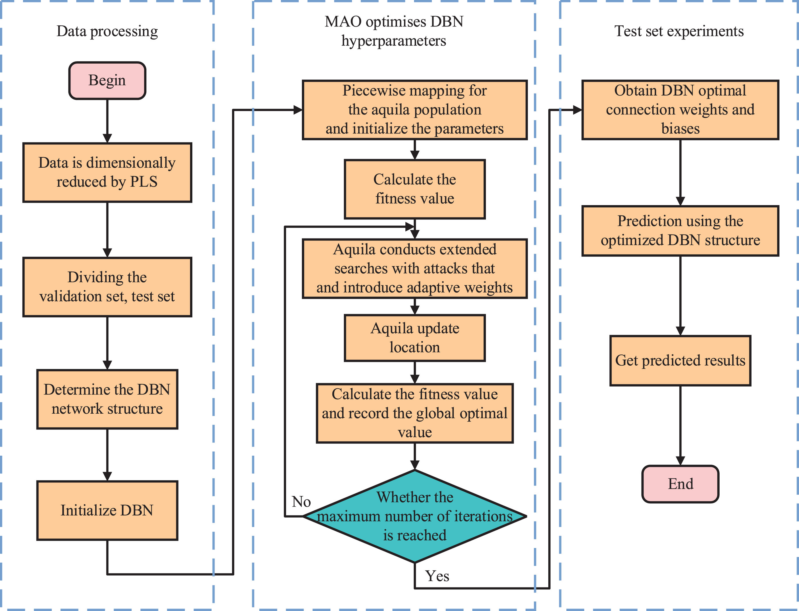
Flow chart of MAO-DBN algorithm.

The MAO-DBN-based membrane fouling prediction method can be divided into the following steps:

Auxiliary variable selection and preprocess-ing using PLS downscaling.

Determine the DBN network structure and initialize the relevant parameters.

Initialize the aquila population and introduce segmented mapping to ensure uniform distribution of the population; introduce adaptive weights to improve the convergence speed and prevent falling into local optimum.

The algorithm stops when the maximum number of iterations is reached, the optimal connection weights and bias of the DBN are obtained. The parameter update is given by Equation (29) as follows:

$\begin{matrix} w_{ij}^{t + 1} = w_{ij}^{t} + η_{w} Δ w_{ij} \\ a_{i}^{t + 1} = a_{i}^{t} + η_{a} Δ a_{i} \\ b_{j}^{t + 1} = b_{j}^{t} + η_{b} Δ b_{j} \end{matrix}$ (29) where w is the connection weight matrix, a and b are the bias vectors of the visible and hidden layers, respectively, Δw_ij, Δa_i, Δb_j are the partial derivatives, η _w , η _a , η _b are the learning rates, and t is the number of iterations.

(5) It is evaluated by substituting it into the training and test sets to obtain the prediction results.

5 Experiments and simulations

This section primarily focuses on comparing the predictive performance of different models through simulation experiments. Firstly, we establish the network architecture. Secondly, various evaluation metrics are used to compare the model with other commonly used soft measurement models, aiming to validate its advantages. Lastly, white noise is introduced to the data to simulate real working conditions, enabling a comparison of prediction accuracies.

5.1 Experimental results and analysis

The experimental data for this paper is taken from Seong Hoon Yoon’s spreadsheet model [30]. The model employs hollow fiber membrane modules and combines the conventional activated sludge method with high-efficiency membrane separation technology. Whereas the traditional activated sludge process uses secondary sedimentation tanks for solid-liquid separation, membrane bioreactor technology achieves solid-liquid separation by using membrane modules instead of secondary sedimentation tanks. This technology enables a shorter process flow, reduces hydraulic residence time, and enhances resistance to water quality and water shock loads. The model consists of three main components: the aeration tank, the anoxic tank and the membrane tank. To improve prediction accuracy, 500 sets of data were identified for model prediction by PLS downscaling and normalization, of which 350 sets were used for modeling training and the remaining 150 sets for model testing.

In this paper, the implicit layer of the model is set to 3 layers, and the optimal number of neurons in the implicit layer is selected based on the model error and the running time. Based on the experimental method, it is observed that the model achieves the smallest MAE when the number of neurons in the implicit layer is set to 25 (Fig. 8). This indicates that the model performs optimally at this configuration. Therefore, we set the number of nodes in the implicit layer to 25.

Fig. 8

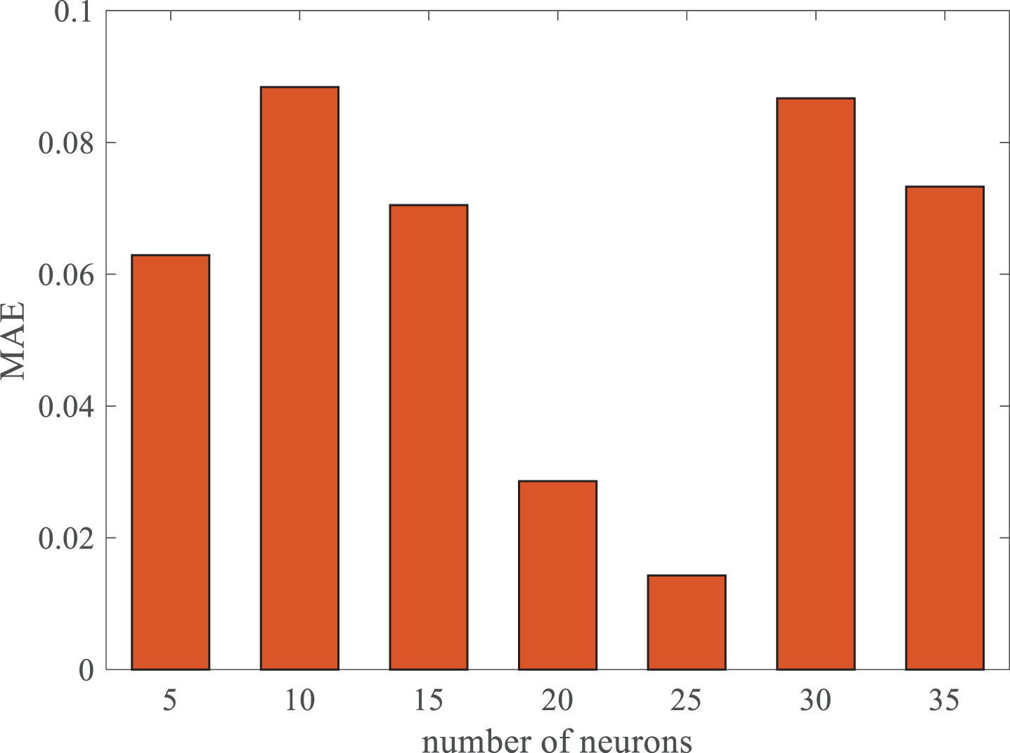
Training effect of different number of neurons.

5.1.1 Evaluation indicators

To provide a more intuitive measure of output accuracy, this paper introduces the following evaluation metrics [31].

(1) Root Mean Square Error RMSE $RMSE = \sqrt{\frac{1}{m} \sum_{i = 1}^{m} {(y_{i} - {\hat{y}}_{i})}^{2}}$ (30)

(2) Mean absolute error MAE $MAE = \frac{1}{m} \sum_{i = 1}^{m} | y_{i} - {\hat{y}}_{i} |$ (31) where y_i is the true value, ${\hat{y}}_{i}$ is the model output value and m is the number of test samples.

(3) Coefficient of determination R² $R^{2} = 1 - \frac{{SS}_{res}}{{SS}_{tot}}$ (32) where SS_res is the error of the regression data against the mean and SS_tot is the error of the true data against the mean.

5.1.2 Accuracy of prediction for various soft measurement models

To compare the advantages of the soft measurement models proposed in this paper, BP, CNN, DBN, SAE, PSO-DBN, WOA-DBN, AO-SAE, AO-CNN, AO-DBN, and MAO-DBN models are used under the same experimental conditions. In contrast, the MAO-DBN model proposed in this paper somewhat outperforms the other models.

Table 3 presents a comparison of the prediction errors for each model. Based on the data in Table 3, the improved soft measurement model reduced RMSE by 94.07% and MAE by 97.66% compared to the shallow BP network under the same experimental conditions. Compared to the DBN model prior to improvement, the improved soft measurement model achieved an RMSE reduction of 88.45% and an MAE reduction of 87.53%. For the PSO-DBN, WOA-DBN, AO-SAE and AO-CNN models, MAE was reduced by 79.62%, 70.45%, 82.8% and 62.85%, and RMSE was reduced by 62.64%, 57.32%, 72.2% and 39.81%, respectively. For the AO-DBN model, the MAE was reduced by 50.46%. The prediction accuracy of the algorithm proposed in this paper reached 98.61%, which is much higher than the accuracy of other algorithms.

Table 3
Comparison of prediction errors

Model RMSE R² MAE

BP 0.7381 0.8505 0.6133

CNN 0.3889 0.9663 0.2687

DBN 0.3785 0.9782 0.1147

SAE 0.3248 0.9798 0.1002

PSO-DBN 0.1170 0.9865 0.0702

WOA-DBN 0.1024 0.9873 0.0484

AO-SAE 0.1574 0.9948 0.0833

AO-CNN 0.0726 0.9912 0.0385

AO-DBN 0.0698 0.9957 0.0283

MAO-DBN 0.0437 0.9991 0.0143

Model	RMSE	R²	MAE
BP	0.7381	0.8505	0.6133
CNN	0.3889	0.9663	0.2687
DBN	0.3785	0.9782	0.1147
SAE	0.3248	0.9798	0.1002
PSO-DBN	0.1170	0.9865	0.0702
WOA-DBN	0.1024	0.9873	0.0484
AO-SAE	0.1574	0.9948	0.0833
AO-CNN	0.0726	0.9912	0.0385
AO-DBN	0.0698	0.9957	0.0283
MAO-DBN	0.0437	0.9991	0.0143

To further evaluate the predictive accuracy and stability, the predicted RMSE values are presented using box plots in Fig. 9. Box plots provide an intuitive visualization of the model’s accuracy and robustness. A lower box plot indicates better predictive accuracy, while a shorter box plot signifies greater stability of the model and more consistent prediction results. It can be observed that the proposed method in this paper demonstrates low prediction errors and exhibits a significant advantage in predictive performance compared to other methods. This indicates that the proposed method achieves high accuracy and possesses excellent stability.

Fig. 9

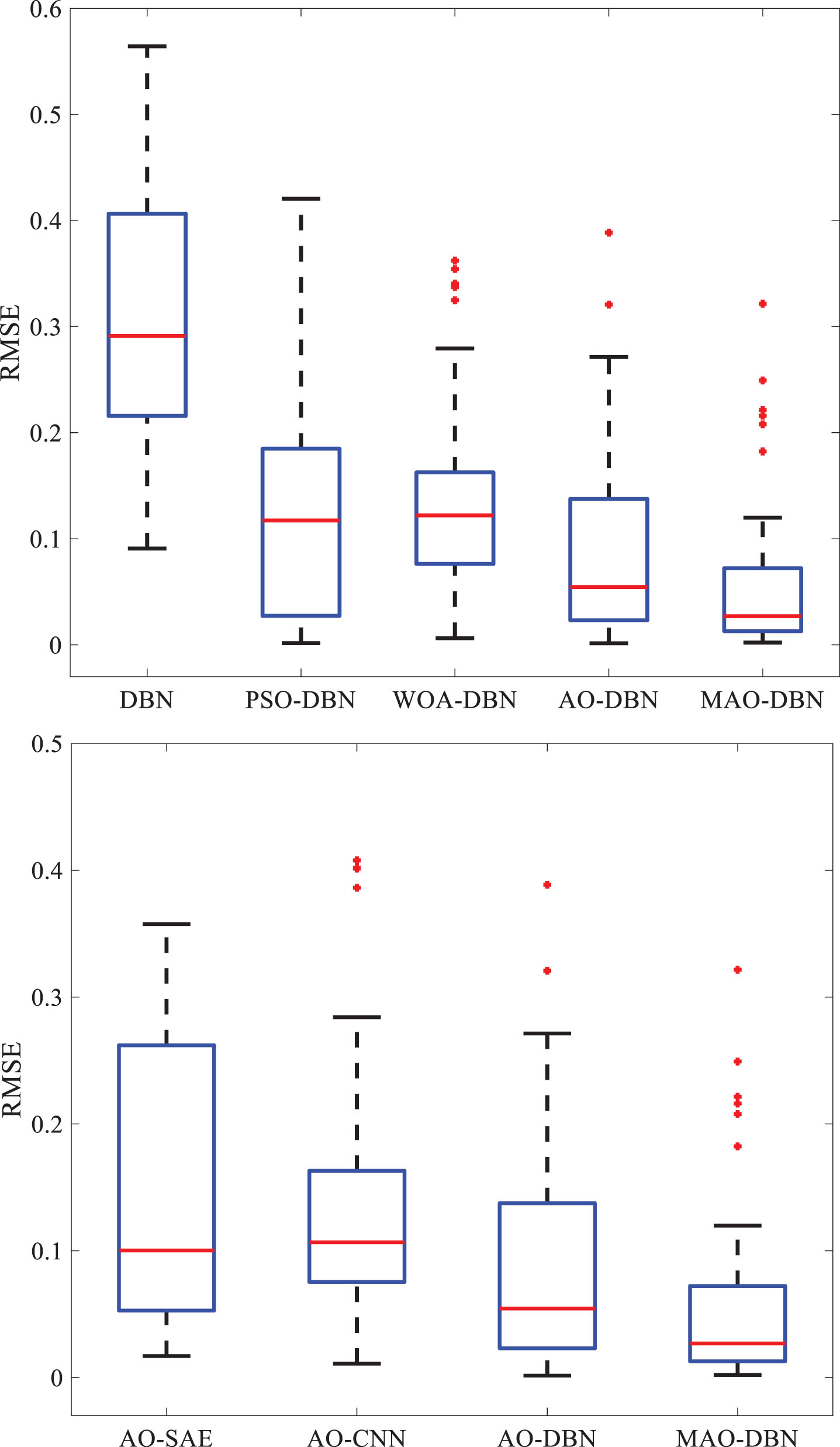
Comparison of RMSE boxplots.

Figure 10 and 11 provide additional insights into the prediction results and error comparisons of each model. From the enlarged view of Fig. 11, it is clear that the model proposed in this paper exhibits minimal error fluctuation, further confirming its high accuracy performance. Overall, the MAO-DBN soft measurement model outperforms other soft measurement models in terms of prediction accuracy across all indicators.

Fig. 10

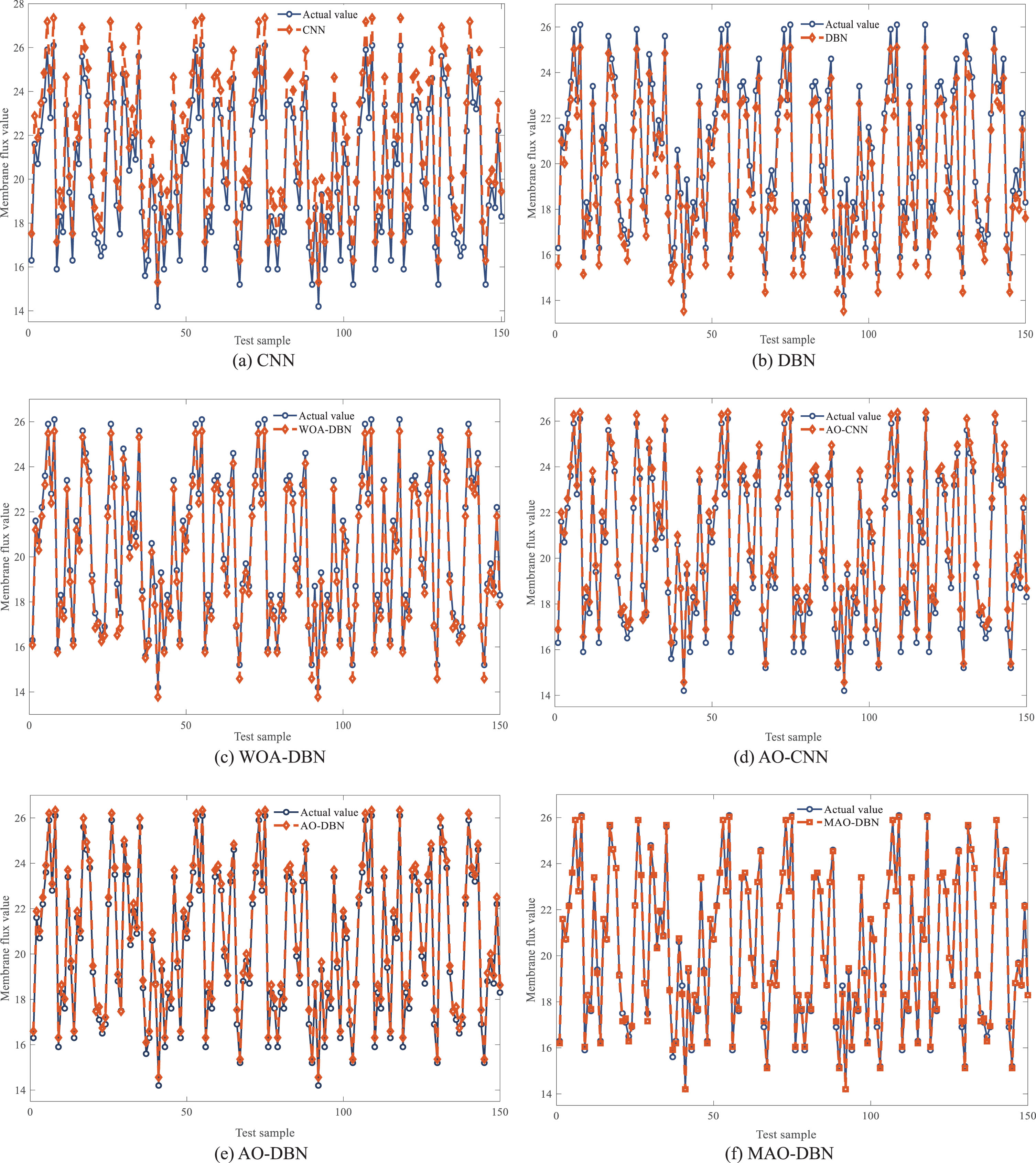
Prediction results of different measurement models.

Fig. 11

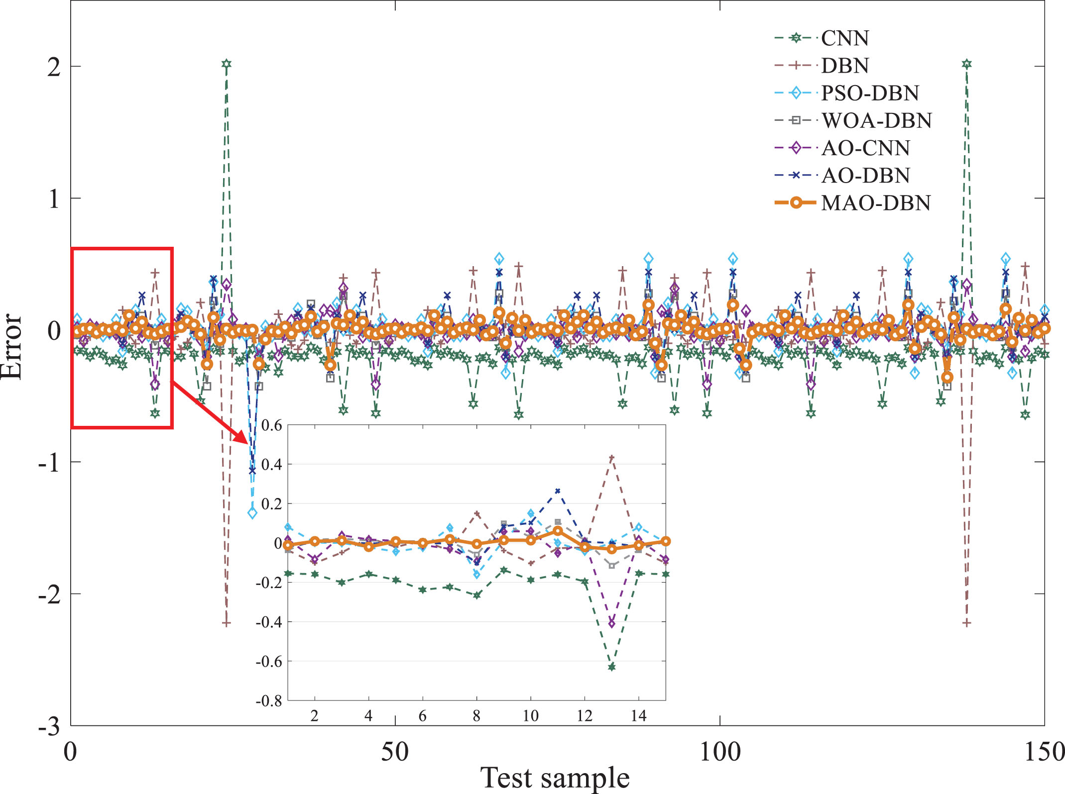
Prediction error curve.

5.2 Performance analysis of noise effects on prediction models

In practice, MBR membrane modules often experience ambient noise during wastewater treatment. Moreover, the membrane modules themselves generate noise, resulting in the collection of membrane fouling data being unnecessarily random. Consequently, it becomes essential to conduct variable noise experiments to predict membrane flux under realistic operating conditions and simulate the uncertainties associated with membrane module operation. In this paper, gaussian noise with Signal-to-Noise Ratios (SNRs) of 2, 6, 8, and 12 dB was introduced to the training samples of membrane pollution data, and various forecasting methods were evaluated accordingly. The experimental results are shown in Table 4.

Table 4
Prediction accuracy at different signal-to-noise ratios

Model Signal-to-noise ratio (in dB)

2 6 8 12

CNN 71.11% 69.15% 70.65% 65.47%

DBN 72.15% 70.24% 76.87% 68.38%

WOA-DBN 87.45% 83.24% 92.24% 81.36%

AO-CNN 88.67% 86.19% 88.16% 88.61%

AO-DBN 91.68% 87.65% 91.58% 90.19%

MAO-DBN 95.26% 93.77% 95.56% 92.72%

Model	Signal-to-noise ratio (in dB)
CNN	71.11%	69.15%	70.65%	65.47%
DBN	72.15%	70.24%	76.87%	68.38%
WOA-DBN	87.45%	83.24%	92.24%	81.36%
AO-CNN	88.67%	86.19%	88.16%	88.61%
AO-DBN	91.68%	87.65%	91.58%	90.19%
MAO-DBN	95.26%	93.77%	95.56%	92.72%

Using Table 4 as a basis for comparison, it is evident that experiments with different SNRs demonstrate a decrease in accuracy for several models. Nevertheless, through longitudinal comparison, it is observed that the MAO-DBN based method consistently outperforms the other methods in terms of accuracy. This finding highlights the effectiveness and reliability of the MAO-DBN approach for membrane flux prediction under varying levels of noise and reinforces its suitability for practical applications.

6 Conclusion

This paper presents a novel MAO-DBN model for predicting membrane fouling, the principal conclusions of this research are outlined below.

PLS is used to reduce the initial auxiliary variables. Additionally, it improves the algorithm’s efficiency and reduces overfitting. To solve the problem of low population diversity in the initial phase of the optimization algorithm, the AO population is initialized using piecewise chaotic mapping. To address the problem that the locally optimal solution is easy to get into trouble with, adaptive weights are used to improve the capability of the algorithm to locate the global optimum. This allows the model to locate the global optimum more efficiently and expeditiously.

In this paper, we propose the MAO-DBN membrane flux prediction model, which demonstrates superior performance in terms of training speed and prediction accuracy compared to other methods. By incorporating multiple membrane fouling factors comprehensively, our improved method significantly enhances the accuracy of predictions. While the MAO-DBN model showcases promising results in the field of membrane fouling, its applicability to other areas remains uncertain. Further investigation is needed to explore its potential in diverse domains, which is a potential direction for future research.

Currently, the selection of the number of hidden layers and the number of neurons in each hidden layer of DBN is usually done by empirical or experimental methods. This method not only increases the workload, but also the complexity or simplicity of the network structure may affect the speed or accuracy. Therefore, a structural self-organizing deep belief network can be designed based on the size and characteristics of the data samples processed to further improve the performance in both prediction speed and accuracy. This will also be the focus of the next research work.

Authorship contribution statement

Zhiwen Wang: Investigation, Methodology, Funding acquisition. Yibin Zhao: Writing review & editing, Investigation, Methodology. Yaoke Shi: Investigation, Methodology. Guobi Ling: Investigation, Methodology editing.

Declaration of competing interest

The authors declare that they have no known competing financial interests or personal relationships that could have appeared to influence the work reported in this article.

Footnotes

Acknowledgments

This work was supported by National Natural Science Foundation of China (62263019). Science and Technology Program of Gansu Province (21ZD4GA028).

References

Hamdhani

, , Eppehimer

D.E.

, , Bogan

M.T.

, , Release of treated effluent into streams: A global review of ecological impacts with a consideration of its potential use for environmental flows[J], Freshwater Biology 65(9) (2020), 1657–1670.

Anonymous. Effects of packing carriers and ultrasonication on membrane fouling and sludge properties of anaerobic side-stream reactor coupled membrane reactors for sludge reduction[J], Journal of Membrane Science 581 (2019), 312–320.

Shi

, , Wang

, , Du

, et al. Membrane fouling diagnosis of membrane components based on multi-feature information fusion[J], Journal of Membrane Science 657 (2022), 120670.

Wang

, , Ng

T.C.A.

, , Ding

, et al. Insights on fouling development and characteristics during different fouling stages between a novel vibrating MBR and an air-sparging MBR for domestic wastewater treatment[J], Water Research 212 (2022), 118098.

Iorhemen

O.T.

, , Hamza

R.A.

, , Tay

J.H.

, , Membrane fouling control in membrane bioreactors (MBRs) using granular materials[J], Bioresource Technology 240 (2017), 9–24.

Nadeem

, , Alliet

, , Plana

, et al. Modeling, simulation and control of biological and chemical P-removal processes for membrane bioreactors (MBRs) from lab to full-scale applications: State of the art[J], Science of The Total Environment 809 (2022), 151109.

Shi

, , Wang

, , Du

, et al. Membrane Fouling Diagnosis of Membrane Components Based on MOJS-ADBN[J], Membranes 12(9) (2022), 843.

Wang

, , Zhang

, , Ma

, et al. Influence of various operating conditions on cleaning efficiency in sequencing batch reactor (SBR) activated sludge process. Part III: Chemical cleaning[J], Desalination 325 (2013), 122–131.

Zhong

, , Yuan

, , Luo

, et al. Water quality prediction of MBR based on machine learning: A novel dataset contribution analysis method[J], Journal of Water Process Engineering 50 (2022), 103296.

10.

Schmitt

, , Banu

, , Yeom

I-T.

, et al. Development of artificial neural networks to predict membrane fouling in an anoxic-aerobic membrane bioreactor treating domestic wastewater[J], Biochemical Engineering Journal 133 (2018), 47–58.

11.

Kovacs

D.J.

, , Li

, , Baetz

B.W.

, et al. Membrane fouling prediction and uncertainty analysis using machine learning: A wastewater treatment plant case study[J], Journal of Membrane Science 660 (2022), 120817.

12.

Mirbagheri

S.A.

, , Bagheri

, et al. Evaluation and prediction of membrane fouling in a submerged membrane bioreactor with simultaneous upward and downward aeration using artificial neural network-genetic algorithm[J], Process Safety and Environmental Protection 96 (2015), 111–124.

13.

Ling

, , Wang

, , Shi

, et al. Membrane Fouling Prediction Based on Tent-SSA-BP[J], Membranes 12(7) (2022), 691.

14.

Jawad

, , Hawari

A.H.

, , Javaid Zaidi

, , Artificial neural network modeling of wastewater treatment and desalination using membrane processes: A review[J], Chemical Engineering Journal 419 (2021), 129540.

15.

, , Behbood

, , Hao

, et al. Transfer learning using computational intelligence: A survey[J], Knowledge-Based Systems 80 (2015), 14–23.

16.

Jiao

, , Huang

, , Ma

, et al. A Model Combining Stacked Auto Encoder and Back Propagation Algorithm for Short-Term Wind Power Forecasting[J], IEEE Access 6 (2018), 17851–17858.

17.

Bahaa

, , Sayed

, et al. A novel hybrid optimization enabled robust CNN algorithm for an IoT network intrusion detection approach[J], 17(12) (2022), e0278493.

18.

Yin

, , Yuan

, , Chen

, et al. High-precision prediction of unionized hydrogen sulfide generation based on limited datasets and its impact on anaerobic digestion of sulfate-rich wastewater[J], Journal of Cleaner Production 341 (2022), 130875.

19.

Niu

, , Yi

, , Chen

, et al. A novel effluent quality predicting model based on genetic-deep belief network algorithm for cleaner production in a full-scale paper-making wastewater treatment[J], Journal of Cleaner Production 265 (2020), 121787.

20.

Abualigah

, , Yousri

, , Abd Elaziz

, et al. Aquila Optimizer: A novel meta-heuristic optimization algorithm[J], Computers & Industrial Engineering 157 (2021), 107250.

21.

Zhang

, , Yang

, , Zhang

, et al. AO-ESN based grounding resistance prediction for offshore wind turbines[J], Journal of Solar Energy 44(05) (2023), 480–486.

22.

, , Chen

, , Li

, et al. Thermal Error Modeling of Spindle for Precision CNC Machine Tool Based on AO-CNN [J], Journal of Xi’an Jiaotong University 56(08) (2022), 51–61.

23.

Hinton

G.E.

, , Osindero

, , The

Y-W.

, , A Fast Learning Algorithm for Deep Belief Nets[J], Neural Computation 18(7) (2006), 1527–1554.

24.

Hinton

, , A practical guide to training restricted boltzmann machines[J], Momentum 9(1) (2010), 926–947.

25.

Han

H.G.

, , Zhang

H.J.

, , Liu

, et al. Data-driven decision-making for wastewater treatment process[J], Control Engineering Practice 96(1) (2020), 104305.

26.

, , Peng

, , Hua

, et al. Research and application of an evolutionary deep learning model based on improved grey wolf optimization algorithm and DBN-ELM for AQI prediction[J], Sustainable Cities and Society 87 (2022), 104209.

27.

Zhang

, , Hua

, , Ji

, et al. An evolutionary robust solar radiation prediction model based on WT-CEEMDAN and IASO-optimized outlier robust extreme learning machine[J], Applied Energy 322 (2022), 119518.

28.

, , Shi

, , Jegatheesan

, et al. A Review on the Mechanism, Impacts and Control Methods of Membrane Fouling in MBR System[J], Membranes 10(2) (2020), 24.

29.

Mihalik

, , Chapman

, , Adams

R.A.

, et al. Canonical Correlation Analysis and Partial Least Squares for Identifying Brain–Behavior Associations: A Tutorial and a Comparative Study[J], Biological Psychiatry: Cognitive Neuroscience and Neuroimaging 7(11) (2022), 1055–1067.

30.

Yoon

S.H.

, Membrane Bioreactor Processes (Advances in Water and Wastewater Transport and Treatment), 1st ed.., CRC Press, Boca Raton, FL, USA, 2020.

31.

, , Gao

, , Cui

, et al. Safety prediction of shield tunnel construction using deep belief network and whale optimization algorithm[J], Automation in Construction 142 (2022), 104488.