An efficient and robust gradient reinforcement learning: Deep comparative policy

Abstract

Recently, actor-critic architectures such as deep deterministic policy gradient (DDPG) are able to understand higher-level concepts for searching rich reward, and generate complex actions in continuous action space, and widely used in practical applications. However, when action space is limited and has dynamic hard margins, training DDPG can be problematic and inefficiency. Since real-world actuators always have margins and interferences, after initialization, the actor network is likely to be stuck at a local optimal point on action space margin: actor gradient orients to the outside of action space but actuators stop at the margin. If the hard margins are complex, dynamic and unknown to the DDPG agent, it is unable to use penalty functions to recover from local optimum. If we enlarge the random process for local exploration, the training could be in potential risk of failure. Therefore, simply relying on gradient of critic network to train the actor network is not a robust method in real environment. To solve this problem, in this paper we modify DDPG to deep comparative policy (DCP). Rather than leveraging critic-to-actor gradient, the core training process of DCP is regulated by a T-fold compare among random proposed adjacent actions. The performance of DDPG, DCP and related algorithms are tested and compared in two experiments. Our results show that, DCP is effective, efficient and qualified to perform all tasks that DDPG can perform. More importantly, DCP is less likely to be influenced by the action space margins, DCP can provide more safety in avoiding training failure and local optimum, and gain more robustness in applications with dynamic hard margins in the action space. Another advantage is that, complex penalty for margin touching detection is not required, the reward function can always be brief and short.

Keywords

Actor-critic deep reinforcement learning intelligent agent iterative learning

1 Introduction

Highly developed in the last decade, reinforcement learning (RL) shows outstanding progress in artificial intelligence [1, 2], as well as nearby areas such as advanced robot [3 –5], game agent [6 –9], word translation [10], dialogue [11 –13] and advertisement [14]. The fundamental concept of RL is to optimize the overall reward within an episode, observing and interacting the outside environment by a state-to-action close loop, which belongs to a problem of Markov decision process (MDP). From 2016, DeepMind [15] technology begins to design and implement powerful deep neural networks on RL tasks, namely as deep reinforcement learning (DRL). Compared with previous RL based on models, DRL is able to perform a model-free approach to arbitrary nonlinear systems, but also it is efficient to derive and store complex action-value function. Besides, DRL directly leverages neural networks to analyse the state space, reducing the ambiguity induced by man-made definition of state patterns. The DRL intelligence enables machines to learn, summarize, predict and act automatically in unknown environment.

To solve a MDP problem, model-based RL, such as AlphaZero [16], tries to learn an environment model describing the possible transition from previous state and action to the reward and next state. When the RL model is closed enough to the real system, without any further actions to attempt, we can use greedy dynamic planning algorithms to find the optimal policy. However, model-free RL shows a comprehensive system model is not necessary for the MDP problem. Instead, the sum of future reward can be estimated by an expectation of action-value function defined by Bellman equation. The action-value function can be updated by temporal difference methods literately or Monte Carlo methods periodically. If we can estimate the action-value function accurately, the policy to reward optimum can be determined. Although model-free RL is unable to predict the state transition, they are adaptive and robust to be implemented. Hence, model-free RL, such as DDPG [17], DQN [15], PPO [18], and A3 C [19], has a wider development than model-based RL.

Classified by the form of agent output, there are two types of RL: value-based RL and policy-based RL. Value-based RL, such as DQN [15 , 20–23], aims to find a distribution of reward in state-value space, approached by a neural network. The output of the network lists out the probable reward after different actions in current state. Policy-based RL, such as DPG [24] and PPO [18], aims to build a direct state-to-action policy with a neural network. The network can generate appropriate actions to gain optimal reward when a state is fed into the agent. Value-based DRL shows excellent performance in playing most games, but it also has limitations when comparing with policy-based RL: (i) It is difficult to implement value-based DRL to tasks with continuous action space. For instance, in mechanical robot control, the joint angles are not convenient to be described in a discrete form. (ii) It is difficult to implement probabilistic policy on value-based RL, in which the action space is fixed and limited, and not convenient to be explored. However, policy-based RL is also challenged by issues such as local optimal converge. Therefore, a new series of method namely actor-critic methods, such as DDPG [17], and its expanded version A3 C [19], are proposed by combining advantages of value-based RL and policy-based RL. Inside actor-critic methods, the output of the actor network is also the input of critic network. The critic network works as an approximator of the action-value function, and the actor network is trained to optimize the reward. The two networks collaborate together, forming a complete agent for model-free learning, which is able to handle most of continuous tasks.

Demonstrated by lots of real-world practical applications, continuous DRL shows promising performance in recent tasks such as robot behavior generation [25, 26], dynamics control [27] and navigation [28]. DRL agent becomes appealing because researchers begin to pay more attention to the intelligence, autonomous performance and the adaptation ability to complex environment. In robot behavior generation tasks, DRL architectures are used to help the robot to respond appropriately at correct timing [29]. Movement can be generated together with coordinate matching, transformation and redundancy reduction optimized, which is believed to have the potential to overcome the challenge of a higher dimensionality in robotics [30]. DRL enables every parameter to be customized for individuals [26] and avoid repetitive offset calibration such as installation errors, friction and centre of gravity. In mechanical dynamics control, DRL improves the property in optimization of gain values for model-based controllers [31] by deeply exploring the prior knowledge. Gain values for force feedback or flight dynamics can be modified context-dependently by the internal neural network, the result has a more vibrationless performance and can provide adequate stability [32]. Without DRL, the partial derivatives coefficients in dynamics would be hard to measure because they depend on the cross effects of many factors and some deflects that have not been considered during design. In navigation and path planning tasks, since model-free RL learns outside environment as a black-box test, navigation problems can also be addressed more efficiently than online trajectory planning [33]. The parameters can slightly adjust and constantly compensate for changing of known and unknown factors while optimizing the movement output.

However, some issues are found during the practical implementation of continuous actor-critic DRL. In real-world applications such as DDPG, the action space of an actuator is often limited, and could has hard margins when the actuator reaches its maximum length, angle, speed, etc. Although we can use reward function to punish the margin to avoid reaching its limitation, when the actor dimension is high, the margin can be dynamic and hard to measure by a simple function, e.g., assembling interference. In this condition, penalty functions are too complicated to be used. Besides, the margins can be unknown in some tasks, whether touching the obstacles is unknown to the DRL agent. In this condition, even using random process for local exploration, the actuator cannot exceed the margin and the exploration could not get rid of local optimum. Since DDPG uses local gradient to update parameters, in the initial training, the training is likely to be stuck at a point on the action space margin to come to a local optimum converge: The gradient forces the action output to move towards the outside of the action space but the actuators stop at the margin, while the error is unknown to the DRL agent. If we use a too large random process for local exploration, the training could be in potential risk of failure. Therefore, DDPG lacks robustness and discussions in dealing with complex, dynamic and unknown margin.

Therefore, to solve this problem and obtain a more robust and normalized DRL architecture, in this paper, we modify DDPG to DCP. We retain the overall duel-network architecture, but the core parameter update process is changed: Rather than leveraging critic-to-actor gradient, the training of DCP is regulated by a T-fold compare among random proposed actions around the actor network. Because of the modification, DCP shows notable novelties in three aspects:

More safety and robustness in training: DCP is less likely to be influenced by action space margin or converge to local optimum, the accuracy and success rate is demonstrated to be robust and stable.

Larger range of random process: To avoid local optimum, the variance of the local random exploration is robust and can be extremely as large as the whole action space, while the training of DCP is less likely to be failed.

Convenient reward function: Even in complex tasks, the reward function for DCP can always be brief and short, since penalty function for margin touching detection is not necessary.

To valid DCP and compare to related algorithms, we have design two experiments to demonstrate its performance to function on different models. The former task is a blind navigation task to avoid barrier walls, which is suitable for rescue inside buildings. The map is unknown to the DRL agents and the agents should reach the goal with high accuracy and low time consumption. The results show that, the DCP has higher accuracy than DDPG and less influenced by the action space margin, but also DCP has an improved robustness in using large random process and different reward functions. The latter experiment is a game of badminton singles with hard margins in the field. Each player is modeled by a collaboration of three DRL agents, controlling ball catching, ball serving and location reset. Rules and environment of the game are similar to the reality. The final scores show that DCP has an obvious advantage from DDPG especially in ball serving. The game also demonstrates the collaborative performance of combining multiple DCP agents.

2 Methods

2.1 Deep deterministic policy gradient (DDPG)

Developed from family of policy gradient (PG), DDPG [17] is able to solve DRL problems with continuous state and action space. Discrete problem can also be solved by adding a softmax layer after the network output. In the training of DDPG, a replay buffer saves the transition from a state to the next state, recording the action history and reward on each time step. Each action is added with a small random process to prevent local optimum. The critic network is trained by the reward expectation from Bellman equation: the current reward with a discounted future reward, shown in Equation (1).

$\begin{matrix} r_{i} + γ Q^{'} (s_{i + 1}, P^{'} (s_{i + 1} | θ^{P^{'}}) | θ^{Q^{'}}) \\ \leftarrow Q (s_{i}, a_{i} | θ^{Q}) \end{matrix}$ (1)

The actor network is trained by firstly taking the action gradient ∇_a of the critic network Q, shown in Equation (2). The gradient propagates back to the input of critic network, and then become the output gradient ∇_θ^P of the actor network P by the chain rule.

$\begin{matrix} \nabla_{θ^{P}} J \approx \frac{1}{N} \sum_{i} \nabla_{a} Q (s, a | θ^{Q}) |_{s = s_{i}, a = P (s_{i}) + R} \\ \nabla_{θ^{P}} P (s | θ^{P}) |_{s_{i}} \end{matrix}$ (2)

Hence, the parameters in actor network can optimize the output of critic network by gradient ascent. But a small difference is, the gradient of actor network ∇_θ^P is derived by the action without the random a = P (s_i), while the gradient of critic network ∇_aQ is derived by the action with the random $a = P (s_{i}) + R$ . DDPG assumes this difference is small. To guarantee converge, DDPG uses slow-updating copies of the two networks to perform soft update, shown in Equation (3). $\begin{matrix} θ^{Q^{'}} \leftarrow τ θ^{Q} + (1 - τ) θ^{Q^{'}} \end{matrix}$

$θ^{P^{'}} \leftarrow τ θ^{P} + (1 - τ) θ^{P^{'}}$ (3)

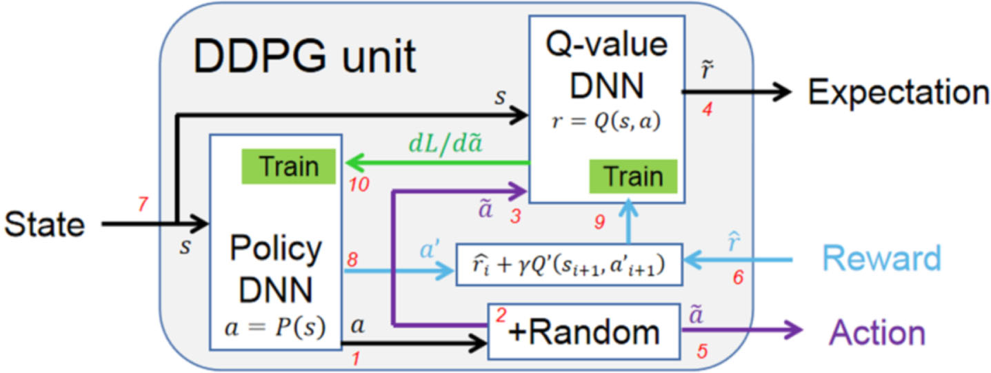
Figure 1 shows a complete training sequence within a time step:<1 > Action a_i is generated by the actor network P after a state s_i is received.<2 > The action a_i is added with a random process, then comes to $\tilde{a_{i}}$ .<3 > Action $\tilde{a_{i}}$ with the state s_i is sent to the critic network.<4 > The expectation $\tilde{r}$ is estimated by the critic network Q.<5 > Action $\tilde{a_{i}}$ is sent to actuators.<6 > The reward $\hat{r_{i}}$ is received.<7 > New state s_i+1 is received.<8 > New action $a_{i + 1}^{'}$ is generated by the actor network copy P′.<9 > Bellman equation (1) is used to train the critic network Q.<10 > Policy gradient (2) is computed to train the actor network P.

Fig. 1

Function diagram of the DDPG in training mode. The index 1 to 10 is correspond to the sequence of training within a time step. Train, collecting training data points.

2.2 Deep comparative policy (DCP)

Based on DDPG, we modify DDPG to DCP. Briefly shown in Fig. 2, state s and action $\tilde{a}$ are vectors linking the agent to the outside environment, reward $\hat{r}$ and expectation r is a single value. The Q-value network Q is named as the critic network, also namely Q network, the Q-value network works as an approximator of the action-value function, which estimates the reward expectation of the current action. The policy network P is named as the actor network, also namely P network, the policy network constantly transform current state into action to gain the optimal expectation. In the training mode of the DCP, the action output a_i is mixed with random to explore nearby action space. After the action $\tilde{a_{i}}$ is is sent to actuators, the reward $\hat{r_{i}}$ can be received from the outside environment. The training the Q-value network is similar to DDPG, shown in Equation (4) to Equation (5). Following Bellman equation, the reward is combined with a discounted future reward estimated by the slow-update copies P′ and Q′ of the both P, Q networks.

Fig. 2

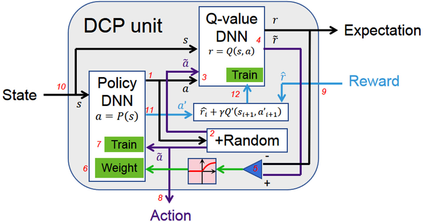
Function diagram of the DCP in training mode. The index 1 to 12 is correspond to pseudo code of the algorithm steps from 1 to 12. Weight, weighted factor for each data point. Train, collecting training data points.

$a_{i + 1}^{'} = P^{'} (s_{i + 1} | θ^{P^{'}})$ (4)

$\hat{r_{i}} + γ Q^{'} (s_{i + 1}, a_{i + 1}^{'} | θ^{Q^{'}}) \leftarrow Q (s_{i}, \tilde{a_{i}} | θ^{Q})$ (5)

However, the update of the actor network P is based on a T-fold compare of the expectation: After an action a_i is generated by the actor network, the random action $\tilde{a_{i}}$ are proposed T times with its expectation $\tilde{r_{i}}$ computed by the critic network Q. Among these random proposed actions, the random action $\tilde{a_{i}}$ with the highest expectation $\tilde{r_{i}}$ is compared and selected. Then, highest expectation $\tilde{r_{i}}$ is compared to expectation r_i of the original action a_i. If $\tilde{r_{i}}$ is better than r_i, $\tilde{a_{i}}$ will be collected as a training data point of the actor network, shown in Equation (6).

$\tilde{a_{i}} \leftarrow P (s_{i} | θ^{P})$ (6)

Depending on the value that $\tilde{r_{i}}$ surpasses r_i, we use a weight factor α_i to modulate the learning rate for individual data points. The weight factor α_i for data point $\tilde{a_{i}}$ is derived by a filter function g, shown in Equation (7) to Equation (8). Large advantage $\tilde{r_{i}} - r_{i}$ would gain a large weight factor in parameter update.

$α_{i} = α_{0} \cdot g (\tilde{r_{i}} - r_{i})$ (7)

$g (r) = {\begin{matrix} 0, r ⩽ 0 \\ \frac{r}{r + 1}, r > 0 \end{matrix}$ (8)

Therefore, the training of the actor network does not rely on the gradient ascent from the critic network. Instead, the parameter update of the actor network is substantially driven by the advantage $\tilde{a_{i}} - a_{i}$ . Since there is no limitation on the variance of the random exploration, the proposed random action $\tilde{a_{i}}$ can be as large as the whole action space. In this case, the training of the critic network can be viewed as global mapping of the action-value function by uniformed random attempts, which is recommended in the initial phase of DCP training. After the critic network is well-trained, the advantage $\tilde{a_{i}} - a_{i}$ would stably guide the actor network to the global optimum point. The training of both actor and critic networks can not only be operated on the same time to perform online gradual leaning, but also can train the actor network offline after the critic network. The T-fold leaning mechanism and the large random exploration ensures DCP more likely to get rid of the local optimal point. Hence, DCP is less likely to be stuck at the action space margin, complex margin penalty function is not required.

In the training of DDPG, the actor network is updated by the gradient ∇_aQoriginated from the output layer of the critic network. The gradient passes back through the whole network to the input layer of the critic network. Then the gradient comes to the output layer of the actor network ∇_θ^PP, and passes back through the whole actor network. However, in tasks with very deep layers, the training has more risk of divergence, vanishing gradient and time consuming. In comparison, the training of DCP actor network does not rely on the gradient from the critic network, the two networks can be trained separately. Hence, DCP has smaller risk and more robustness in large-scale network training.

Algorithm 1: DCP
Randomly initialize online critic network Q (s, a\|θ^Q) and actor network P (s\|θ^P) with weights θ^Q andθ^P.
Initialize target network Q′ andP′ with weights θ^Q′ ← θ^Q,θ^P′ ← θ^P.
For each episodes
Reset actuators.
Receive initial observation states₁.
Do
(step 1) Generate actiona_i = P (s_i\|θ^P).
For T-times find the maximum $\tilde{r_{i}}$
(step 2) Add random $\tilde{a_{i}} = a_{i} + N$ within action space.
(step 3 & 4) Estimate expectation $\tilde{r_{i}} = Q (s_{i}, \tilde{a_{i}} \| θ^{Q})$ .
End for
(step 4) Estimate expectation r_i = Q (s_i, a_i\|θ^Q).
If $\tilde{r_{i}} > r_{i}$ (step 5) Compare
(step 6) Compute adaptive weight $α_{i} = α_{0} \cdot g (\tilde{r_{i}} - r_{i})$ for actor network learning.
(step 7) Train actor $\tilde{a_{i}} \leftarrow P (s_{i} \| θ^{P})$ with minibatch.
End if
(step 8) Action output $\tilde{a_{i}}$ .
DCP unit task suspend (CPU can do something else).
(step 9 & 10) Wake up when DCP receive reward $\hat{r_{i}}$ and next states_i+1.
(step 11) Estimate $a_{i + 1}^{'} = P^{'} (s_{i + 1} \| θ^{P^{'}})$ by target network P′.
(step 12) Train critic network $\hat{r_{i}} + γ Q^{'} (s_{i + 1}, a_{i + 1}^{'} \| θ^{Q^{'}}) \leftarrow Q (s_{i}, \tilde{a_{i}} \| θ^{Q})$ with minibatch.
i = i + 1
While (state within valid range)
Update the target network.
θ^Q′ ← τθ^Q + (1 - τ) θ^Q′
θ^P′ ← τθ^P + (1 - τ) θ^P′
End for

To implement DCP, there are five steps: (i) Depending on the requirement of the task, the structures of online networks P and Q should be selected. The layer width and depth should be able to handle the complexity of the task, but should not be too large, otherwise it would be under-fitting. The neural networks can be initialized to random following an uniform distribution of $(\frac{1}{\sqrt{v}}, - \frac{1}{\sqrt{v}})$ , where v denotes the length of the input of that layer. (ii) The network copies P′ and Q′ are created. The rate τ of P′ and Q′ network updating should be selected, which is 0.01 by default. During training, the parameters of online networks P and Q are updated in each loop, P′ and Q′ should be constantly and gradually updated by τ. (iii) Hyperparameter T and γ should be selected before training. The value of T and γ is depending on the different tasks. If the action-value function is complex, T should be increased. If we only want to optimize single-shot reward, γ can even be set to 0. The default configuration for T and γ is 4 and 0.7. (iv) All environment initialization is ready, actuators are reset to initial state. Then follow the program in the Algorithm 1 above. The DCP agent will generate actions, then compare actions, train the actor network and give action output. After DCP receives the reward, DCP can train the critic network. (v) The algorithm will always check whether the system stays within valid range. If not, the algorithms should stop the training and reset to initial state. After networks P and Q are well-trained, in the testing mode, the system directly outputs the action a_i without random, attached with an expectation of reward r_i.

3 Experiment 1: Path planning

3.1 Experimental configurations

3.1.1 Task environment

The following two experiments demonstrate the DCP and make comparison with related algorithms. In the first experiment, we design a simple case of path planing task. Path planing is important and often used in applications of robot navigation to avoid obstacles. Similar to rescue inside buildings, the task is to perform a blind navigation between labyrinthine walls to get to the center. We have tested the performance of our DCP with DDPG, PPO and DQN. The shape of the wall is shown in Fig. 3, which is unknown to the DRL agents. The DRL agent should pass through the gaps between walls and move onto the center. Since this is a blind navigation task, the agents can only know the coordinates on the map by inertial measurement units or position system like GPS. In each task, the origin is randomly selected on the stage boundary of 6 units. The thickness of the walls is 0 unit. When the agent moves toward the walls, the walls can create dynamic hard margins in the agent’s action space: We assume that only the movement component paralleled to the wall is allowed, the vertical movement component is blocked. Besides, whether touching the wall is unknown to the agent.

Fig. 3

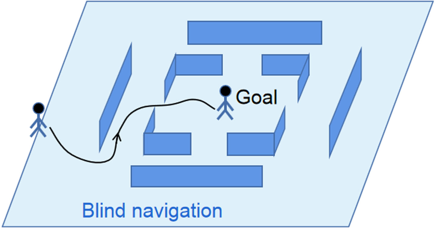
Path planning task. The shape of the barrier walls is unknown to the DRL agents. The walls can create hard boundaries in the agent’s action space, and the boundaries vary in different locations.

Both DDPG agent and DCP agent has a duel-networks architecture. The PPO agent and DQN agent only contains the actor network. Their actor network and critic network are the same but trained in different ways. The input of the actor networks includes the location coordinates x, the network output includes the movement on each coordinate Δx, described by an increment vector, shown in Equation (9).

$Δ x = P (x)$ (9)

The input of the critic network in Equation (10) is formulated in a form of the action-value function.

$r = Q (x, Δ x)$ (10)

3.1.2 Reward functions

All the networks use the same depth with the same hidden layer length. We test the scale from 2 hidden layers by 32 layer length to 6 hidden layers by 64 layer length, which is sufficient for the function requirement of the task. The reward for the DRL agent is given by three ways. Equation (11) is the local reward (LR), which estimates the advantage in a single step action. LR will become negative if the agent moves away from the center, vice versa. Equation (12) is the global reward (GR), which estimates the overall progress after a single action step. GR measures the negative distance to the center. Equation (13) combines LR and GR, balanced by weight factors. C, C₁ and C₂ are constants which can perform normalization. α_L and α_R are weight factors. All these reward functions contain no punishment from touching walls.

${\hat{r}}_{L} = C \cdot (∥ x_{n} ∥ - ∥ x_{n + 1} ∥)$ (11)

${\hat{r}}_{G} = - C_{1} \cdot ∥ x_{n + 1} ∥ + C_{2}$ (12)

${\hat{r}}_{LG} = α_{L} \cdot r_{L} + α_{R} \cdot r_{R}$ (13)

Since the DQN agent is a discrete actor, we use an 8-options softmax layer on its network output, containing 8 movements of 0.25 unit length in directions of n times 45 degrees, n = 0 to 7. A training episode is ended once the DRL agent crosses the boundary or reaches the center (<0.1 unit) and keeping stable 10 steps, then a new episode begins. The network learning rate for all agents are the same 1/4096, trained for sufficient 3,000 episodes. The L2 regulator rate is 1e-4. Dropout 0.5 is also used.

3.2 Results

3.2.1 The accuracy of DCP is less influenced by the margins

The performance of the four agents is estimated by the error to goal, success rate and time consumption. The error is defined by Equation (14), which is distance from the goal to the location that DRL agent converges.

$e = ∥ x_{end} ∥$ (14)

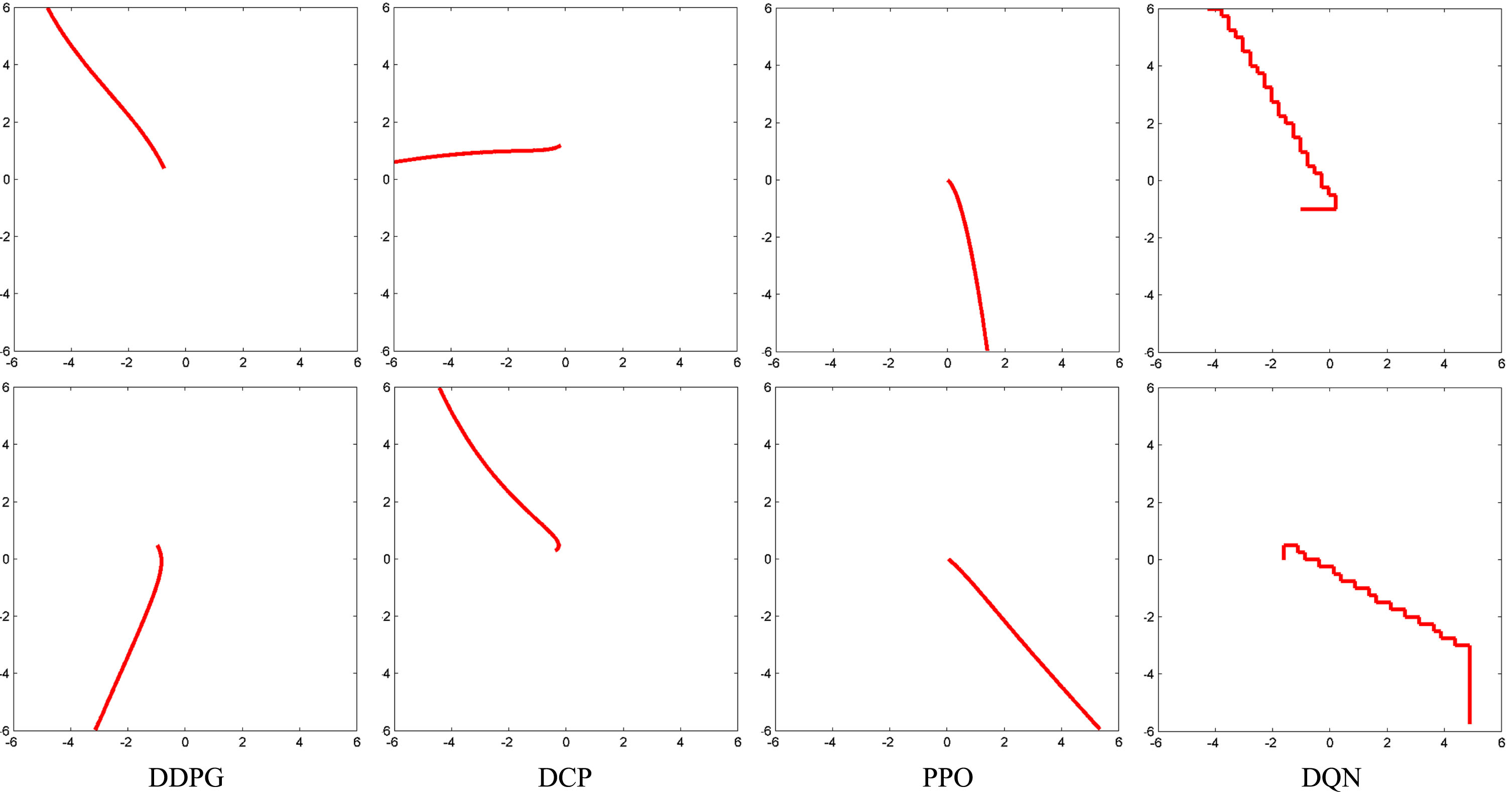
Especially, if the DRL agent converges within a loop around the goal, the error is the averaged distance to the goal. We test each agent for 100 times. Figure 4 shows some trajectories of the four DRL agents. All agents can stop at a stable ending but the DQN agent. DCP and PPO can converge at a location closer to the center than DDPG and DQN. All the agents can roughly find the shortest path towards the goal. Figure 6 upper chart shows the error of all trajectories that successfully reach the goal, stable < 2 units, among the 100 tests. DCP has a smaller error than DDPG. We also test the performance of four agents without the barrier wall in a contrast experiment. Figure 5 shows some trajectories tested without the barrier walls, and again we summarize its error among 100 tests in Fig. 6 lower chart. We find the barrier walls lead to a large error increment in DDPG and DQN. The influence on DCP and PPO is relatively smaller. Hence, the training mechanism of DCP and PPO is better than that of DDPG and DQN, in solving continuous problems with hard action space margins.

Fig. 4

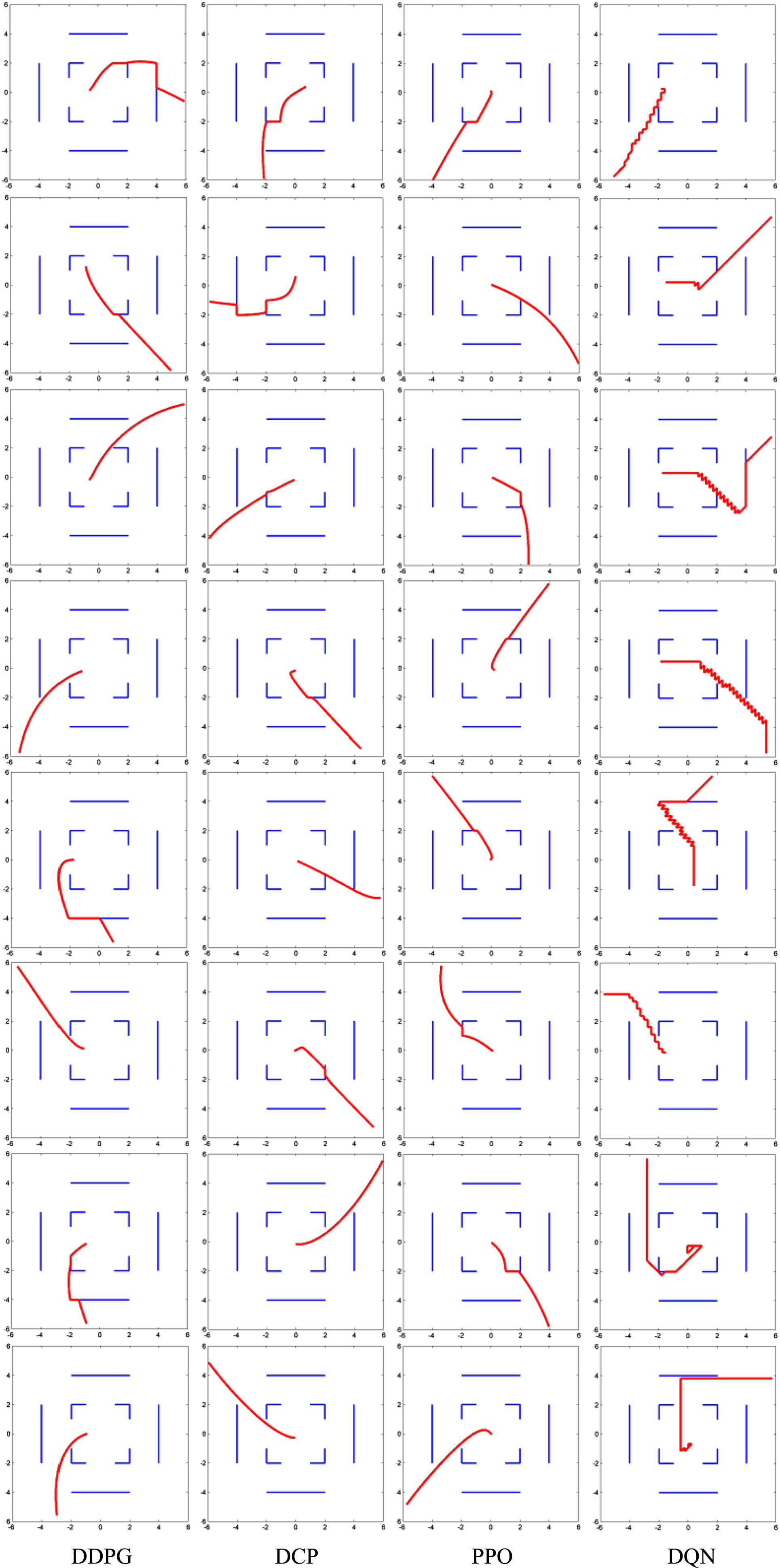
Some trajectories of the four DRL agents.

Fig. 5

Comparison test. Some trajectories of the four DRL agents, tested without barrier walls.

Fig. 6

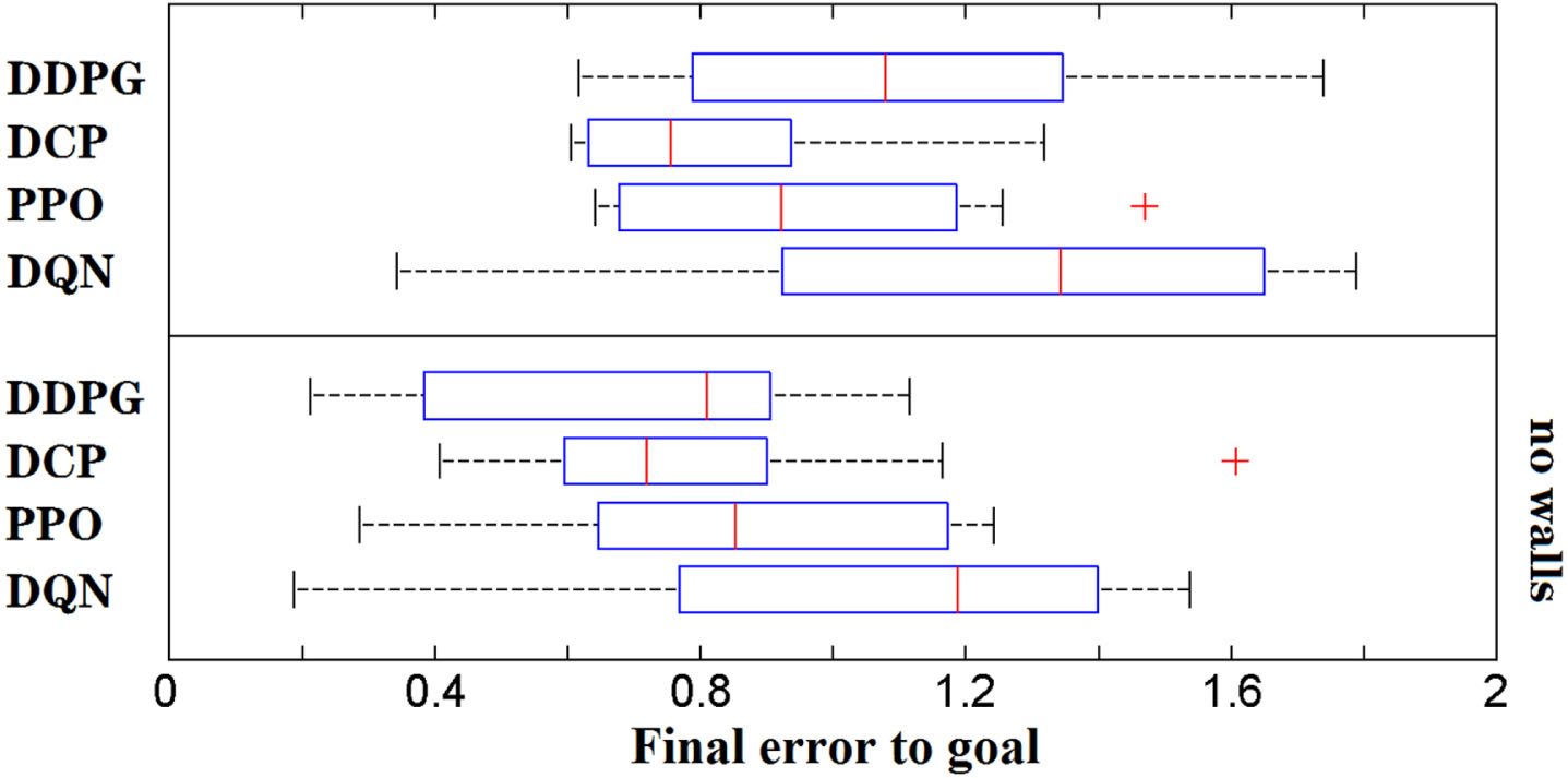
Accuracy of the path planning task. The final error among 100 tests with barrier walls is shown in the upper chart. In comparison, the lower chart shows the final error among 100 tests without barrier walls.

3.2.2 DCP’s T-fold mechanism has the similar effect of critic-to-actor gradient

We summarize the steps which the four agents use to reach the goal among the 100 tests in Fig. 7. The DDPG has the lowest time consumption but the difference between DDPG and DCP is small. Although DCP does not use gradient, to find the shortest way, the efficiency of using T-fold compare to find the steepest ascent way is basically similar to DDPG, which can achieve similar effect of critic-to actor gradient.

Fig. 7

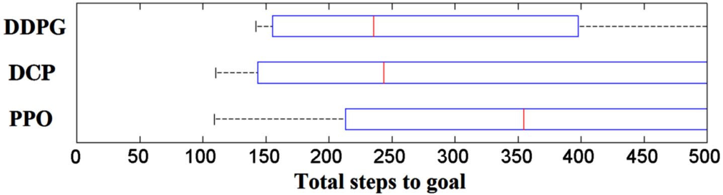
Time consumption of the path planning task. The total time steps among 100 tests are compared between DDPG, DCP and PPO. Since DQN belongs to discrete methods, the comparison may not be reasonable.

3.2.3 The success rate for DCP is high

Due to the parameters initialization and insufficient training, there are still some cases that DRL agents fail to reach the goal. Table 1 lists out the success rate of the four agents, under different network sizes. The DCP has the highest success rate and surpasses DDPG obviously. Among all four agents, the network size over 4×48 is sufficient for the path planning task.

Table 1
Success rate of the DRL agents (using different network sizes)

Agents Hidden layers×layer length

2×32 4×48 6×64

DDPG 85% 89% 90%

DCP 91% 95% 95%

PPO 90% 93% 94%

DQN 88% 91% 90%

Agents	Hidden layers×layer length
DDPG	85%	89%	90%
DCP	91%	95%	95%
PPO	90%	93%	94%
DQN	88%	91%	90%

(Total 100 tests).

3.2.4 DCP can use robust reward functions

We also test how reward function influences the four agents. We train the four agents three times by reward functions Equation (11) to Equation (13), then repeat the test again. The success rate of using the three reward functions is shown in Table 2. The DDPG agent is influenced by reward functions, and its rate decreases when using LR. It indicates that the training is slow and insufficient. In comparison, DCP shows a wider adaptability of different form of reward functions.

Table 2
Success rate of the DRL agents (using different reward functions)

Agents Reward function

GR GR+LR LR

DDPG 89% 82% 71%

DCP 95% 95% 93%

PPO 93% 94% 95%

DQN 91% 90% 87%

Agents	Reward function
DDPG	89%	82%	71%
DCP	95%	95%	93%
PPO	93%	94%	95%
DQN	91%	90%	87%

(Total 100 tests, using 4×48).

3.2.5 DCP is safe to use large random exploration

In DDPG and DCP, the variance of the random exploration process is a hyperparameter that control the efficiency of learning. A large random process can speed up the exploration of the action space. But in DDPG, the random cannot be too large since DDPG assumes $P (s_{i}) + R \approx P (s_{i})$ in Equation (2). However, the training mechanism of DCP is different and does not have such assumption. Table 3 lists out the rate of training failure of the DDPG and DCP agents by using random process ranging from 0.2 to 1. We find the failure rate of DDPG largely increases and the training becomes abnormal when a large random process is used. By contrast, the DCP training is not influenced by the scale of the random process.

Table 3
Rate of training failure (using large random)

Agents Random process

σ² = 0.2 σ² = 0.5 σ² = 1.0

DDPG 0% 33% 96%

DCP 0% 0% 0%

Agents	Random process
DDPG	0%	33%	96%
DCP	0%	0%	0%

(Total 100 tests, using 4×48 GR).

4 Experiment 2: Badminton game

4.1 Experimental configurations

4.1.1 Game environment

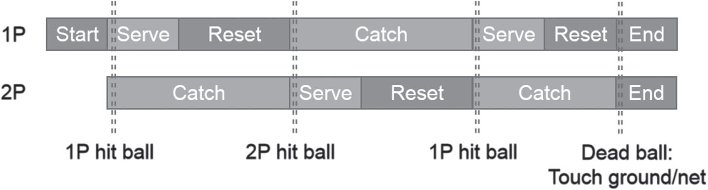
The second experiment is a complex RL application in competitive ball sports. We have tested the performance of the three continuous DRL agents: DDPG, DCP and PPO in playing singles badminton games. Discrete RL methods such as DQN are problematic and hard to implement since a continuous and precise coordinates is required to guide the players to reposition on field, but also an accurate angle is required to make the ball bypass the other player. This experiment builds a virtual coliseum to test the performance of DRL agents. We use standard field of badminton singles, the field has a 3D hard margin of 13.4 meters length and 5.18 meters width. The height of the barrier net between players is 1.55 meters. The trajectory of the ball on air is calculated by numerical simulation considering gravity and squared-speed drag in time step of 0.001 second. A player wins marks while the other player makes a mistake. For instance: failed to catch a ball, serve a ball to the outside or hit the net. A game is ended when either of the players gets more than 10 marks while has 2 marks superior to the other, or either of the players gets 20 marks. Overall, the rules of the game are mostly similar to the reality, but some complicated and professional details are simplified and removed, such as service line and left-right half field switching. Besides, here we assume the maximum ball speed that a player can serve is 77 meters per second. The maximum moving speed of a player is 4.5 meters per second. The maximum radius that a player can catch a ball is 1.3 meters. These simplifications and settings may be slightly different from the real conditions but would not influence our model demonstration.

4.1.2 Multi-agent collaboration

In the second experiment, multiple DRL agents collaborate together to perform the task. Shown in Fig. 8, a complete player is built by three individuals agents, namely the “catch” agent, the “serve” agent and the “reset” agent. The “catch” agent aims to estimate a location on self field to move to after the other player serves a ball, where the player itself can best capture the ball, shown is Equation (15).

Fig. 8

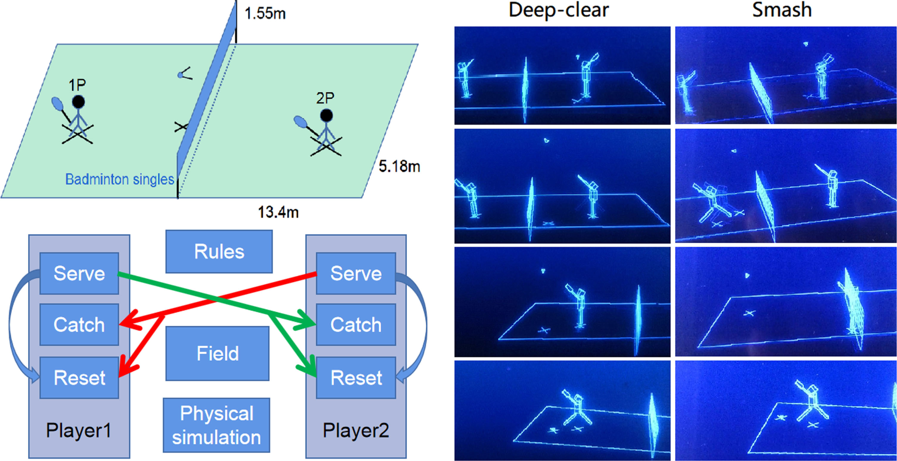
Singles badminton games. The physical environment is simulated by a neural-computing pad. Each player is modeled by the collaboration of three RL agents. Three teams of players trained by DDPG, DCP and PPO participate in the competition.

${l^{'}}_{k} = P_{C k} (l_{k}, x, \dot{x})$ (15)

l_k is the current location of player k. x and $\dot{x}$ are position and velocity of the ball. The “serve” agent is able to provide a velocity ${\dot{x}}^{'}$ to serve a ball after the ball is captured at position x, the ball is served to not be captured by the other player $\tilde{k}$ and landing on the opposite field, shown in Equation (16).

${\dot{x}}^{'} = P_{Sk} (l_{\tilde{k}}, x)$ (16)

Hence, the “catch” agent and the “serve” agent are hostile between players. The “reset” agent helps to predict a location on self field where the player itself are likely to catch next ball after a ball has just served to the other player, shown in Equation (17).

${l^{'}}_{k} = P_{R k} (l_{\tilde{k}}, x, {\dot{x}}^{'})$ (17)

Since the ball has not been captured and served by the other player yet, the “reset” agent operates before the “catch” agent. All input of the three DRL agents contains necessary global information of current game, they are position and velocity of the ball and location of both players. The outputs of the agents control the location of player and ball serving, respectively. The three agents cooperate together but perform different functions at different timings. Compared with the first experiment, the second experiment can test the collaboration performance in solving complex tasks.

4.1.3 Reward functions

The reward function for the “catch” agent is shown in Equation (18), which is a reward plus a Gaussian radial basis function d. C is a constant.

${\hat{r}}_{C} = {\begin{matrix} \begin{matrix} d \\ d - 1 \end{matrix} & \begin{matrix} , ballcaptured \\ , notcaptured \end{matrix} \end{matrix}$ (18)

$d = \exp (- C_{d} \cdot {∥ l_{k} - x ∥}^{2})$ (19)

The reward would become a negative punishment if the ball is failed to be captured. The radial basis function measures the distance from the player to the ball. The reward function for the “serve” agent is shown in Equation (20), which is separated into four conditions.

${\hat{r}}_{S} = {\begin{matrix} \begin{matrix} \begin{matrix} \tilde{d} + h - 4 \\ \tilde{d} - h - 1 \end{matrix} \\ \begin{matrix} 0 \\ 4 - \tilde{d} \end{matrix} \end{matrix} & \begin{matrix} \begin{matrix} , outside \\ , hitnet \end{matrix} \\ \begin{matrix} , capturedby \tilde{k} \\ , notcapturedby \tilde{k} \end{matrix} \end{matrix} \end{matrix}$ (20)

$\tilde{d} = \exp (- C_{d} \cdot {∥ l_{\tilde{k}} - x ∥}^{2})$ (21)

$h = \exp (- x_{z})$ (22)

Both the first and second condition are punishment since they are self mistakes. If a serving ball is captured by the other player, there is no punishment or reward. Only the last condition will have a positive reward. The reward function for the “reset” agent is also the same value of the “catch” agent, since both of them are aimed at catching ball. All reward functions are simple and contain no punishment about whether the agent touches the action space margin. Figure 9 show the sequence chart of the three agents.

Fig. 9

Sequence chart of the three agents.

The game is started by a ball serving by either of players, following by a reset movement. Meanwhile, the other player enters the catching phase. Once captured, two players switch its phases. The game is ended when a dead ball occurs. Then the marks are updated and reward functions are activated.

In each agent, there is an actor network and may have a critic network. Hence, total 12 neural networks are activated during a game. The parameter initialization is similar to the first experiment. All networks use an architecture of 4 hidden layers with 48 layer length. Each training episode is corresponded to a mark, which is from the first ball serving until the ball drops on the ground or net. The network learning rate for all agents are the same 1/4096, trained for sufficient 20,000 episodes. The L2 regulator rate is 1e-4. Dynamic input normalization is updated on every minibatch of 64. Dropout 0.5 is also used.

4.2 Results

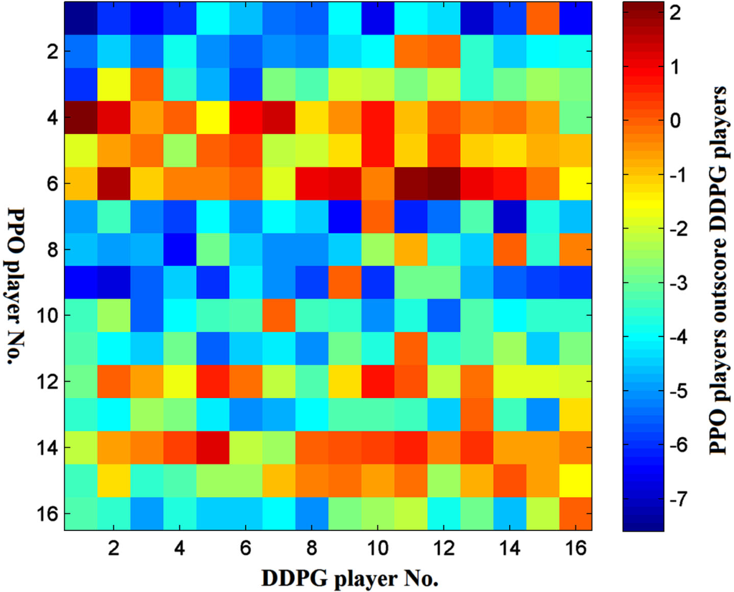
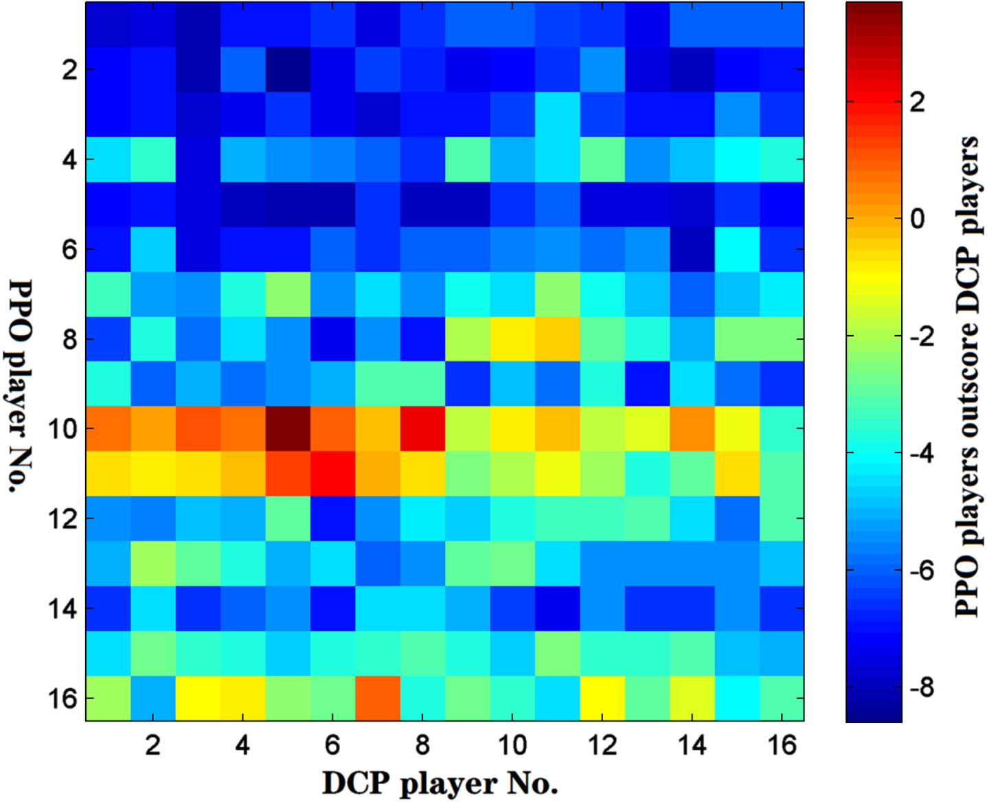
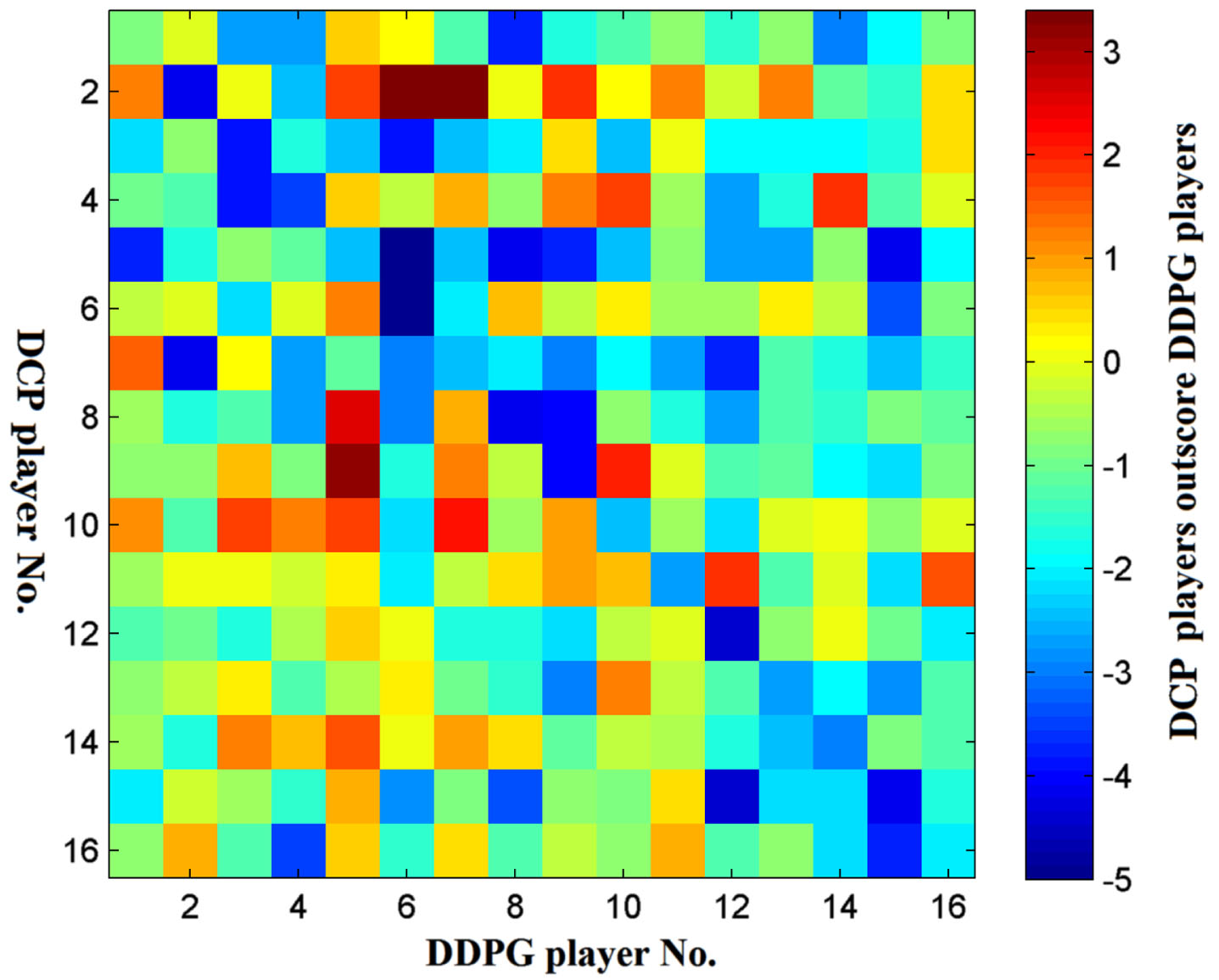
We have trained three teams: DDPG team, DCP teams and PPO teams. Within each team, 16 players randomly take competitions with each other. The standard deviation of the random exploring process of every DRL agents are changed randomly from 0.02 to 0.2 in every games. The performance of each team is estimated by the average score, the success rate of “catch” and the error rate of “serve”.

4.2.1 Overall scores of DCP increase as T increases

We hold three competitions between the three teams: DDPG vs DCP, DDPG vs PPO and DCP vs PPO. The final score of each competition is estimated by the mean of mark difference in 1,024 repeated games. The 1,024 games are organized into 4 repeated games between the 16 players from two different teams. Especially in DCP, we test the effects of the hyperparameter T, which control the level of action space exploration. Therefore, we trained the DCP team three times with T = 1, 4 and 16, respectively. Table 4 shows the overall scores in the competitions between the three teams. We find the PPO team is inferior to the other two teams, with a score difference of larger than 2. The scores contributed by every player are shown in Fig. 10 and Fig. 11. Only few PPO players surpass the DDPG and DCP players. In the competition between DDPG and DCP, Fig. 12 and Fig. 13 shows the scores of every player when

Table 4
Overall scores of the three teams

Player 1 outscores Player 2
Player 1	Player 2
	DCP (T = 1)	DCP (T = 4)	DCP (T = 16)	PPO
DDPG	0.8355	0.0141	–0.6953	2.7039
DCP (T = 16)				4.6875

(The DCP team is trained three times by T = 1, T = 4, and T = 16, based on the same parameter initialization.).

Fig. 10

Scores contribution of each player. (P1 = DDPG, P2 = PPO).

Fig. 11

Scores contribution of each player. (P1 = DCP16, P2 = PPO).

Fig. 12

Scores contribution of each player. (P1 = DDPG, P2 = DCP (T = 1)).

Fig. 13

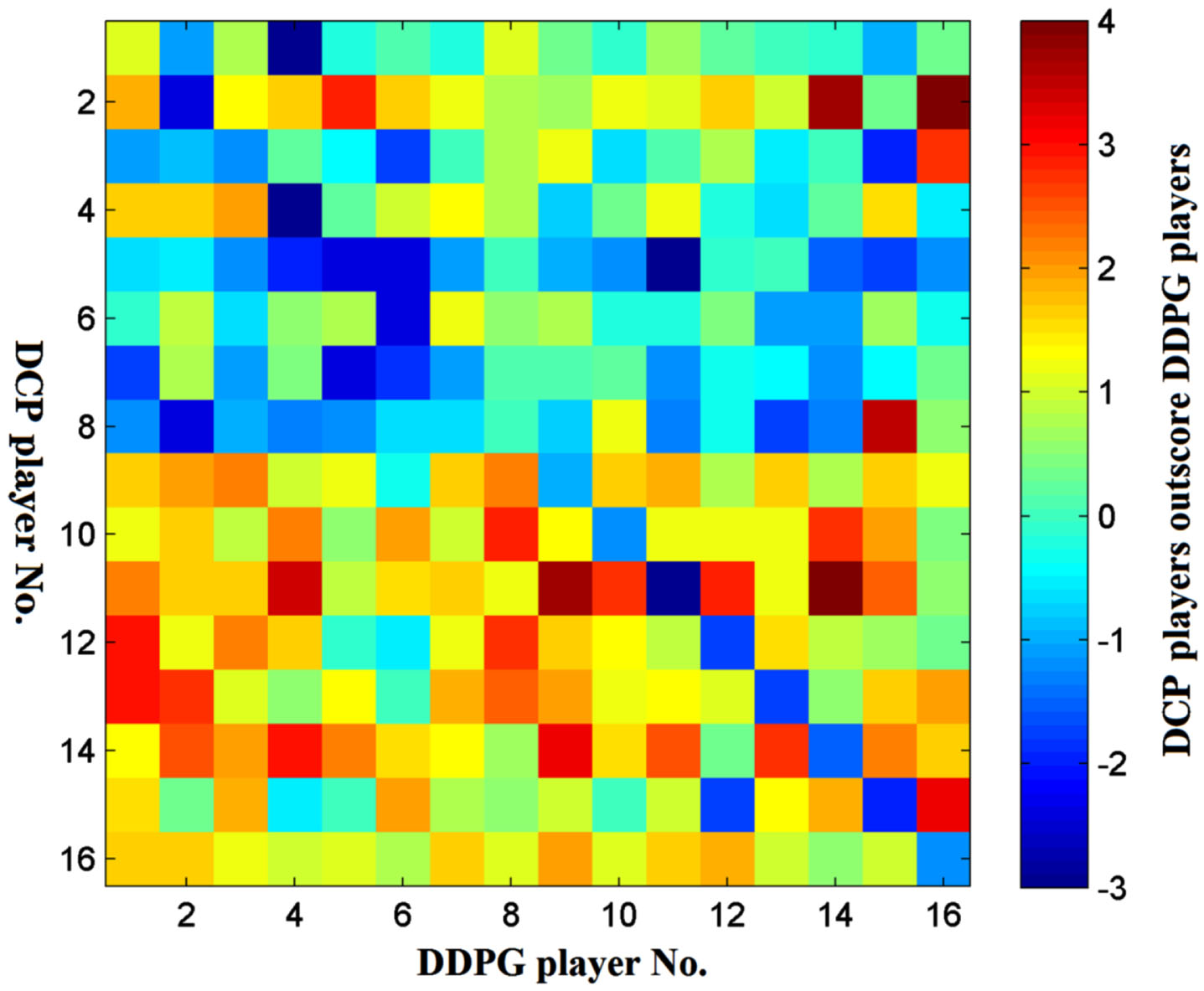
Scores contribution of each player. (P1 = DDPG, P2 = DCP (T = 16)).

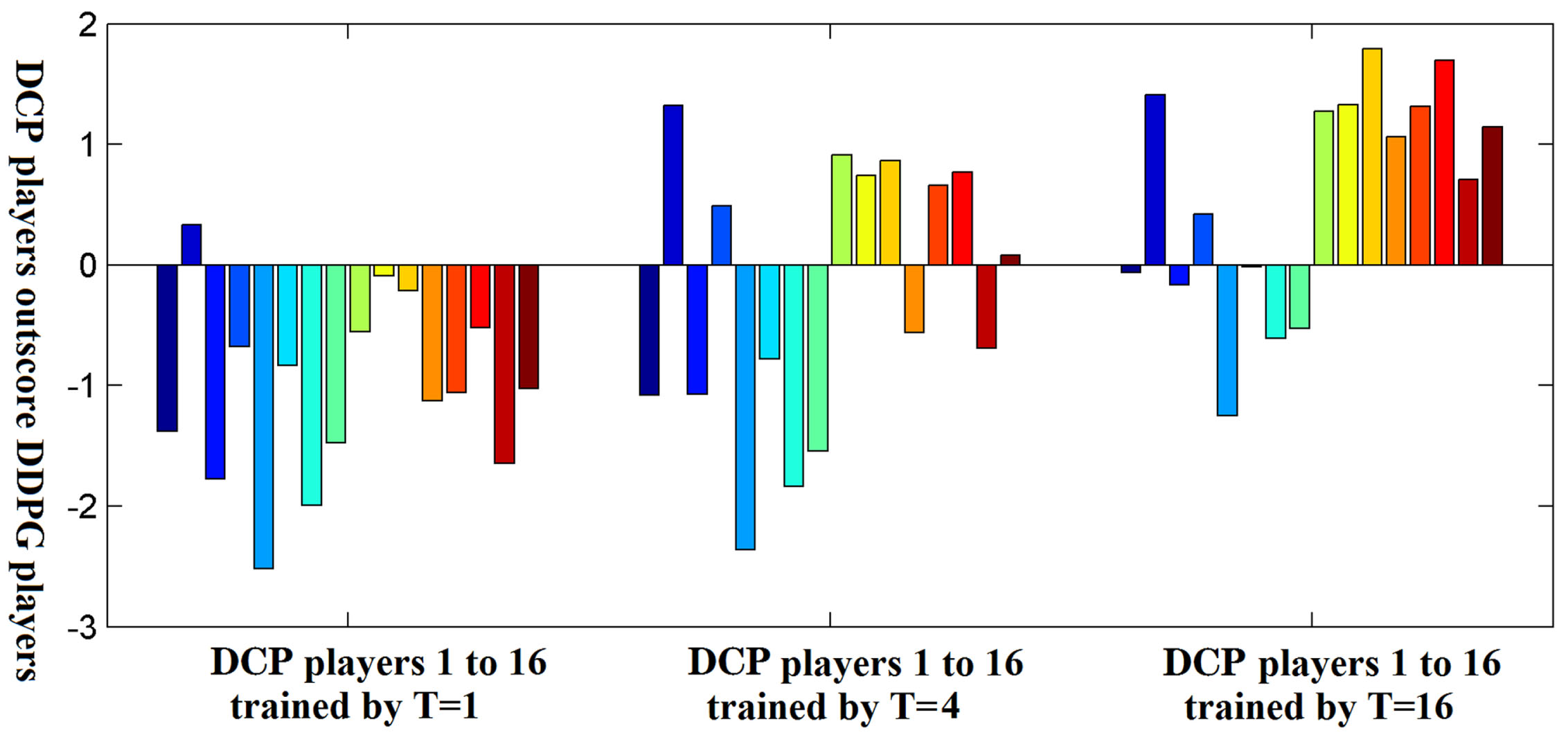
T = 1 and T = 16. Most players from DDPG and DCP match each other in strength. Besides, an overall tendency is, DCP outscores DDPG as the T goes higher. Also shown in Fig. 14, when T is small, the action space exploration is insufficient, the DCP training falls behind DDPG. When T is larger than 4, DCP gradually surpasses DDPG.

Fig. 14

The influence of the hyperparameter T. When T is larger than 4, DCP can gradually surpass DDPG.

4.2.2 DCP can catch difficult balls

The overall scores may not be an accurate estimation since the final performance can only demonstrate the cooperation of the “catch” agent, the “serve” agent and the “reset” agent. A fault can be risen from any of them. Hence, we firstly analyze the performance of the “catch” agent by the success rate by Equation (23). Ball served outside or hitting net is ignored.

$Success rate = \frac{Captured}{Captured + Not captured}$ (23)

After the badminton competition, we test the “catch” agent by an additional ball catching test: one player catching a ball served by the other player. In Fig. 15, the heat map shows the action-value function (Q-value network) in different conditions of players locations and ball position. The hot areas indicate the best locations to capture the ball, learned by DDPG and DCP players. We find the overall shapes are quite similar. Both of them are also consistent to real human decisions. Table 5 lists out the success rate of DDPG players, DCP players and PPO players, respectively. The rate of DDPG and DCP are basically similar and superior to PPO by 5% to 10%.

Fig. 15

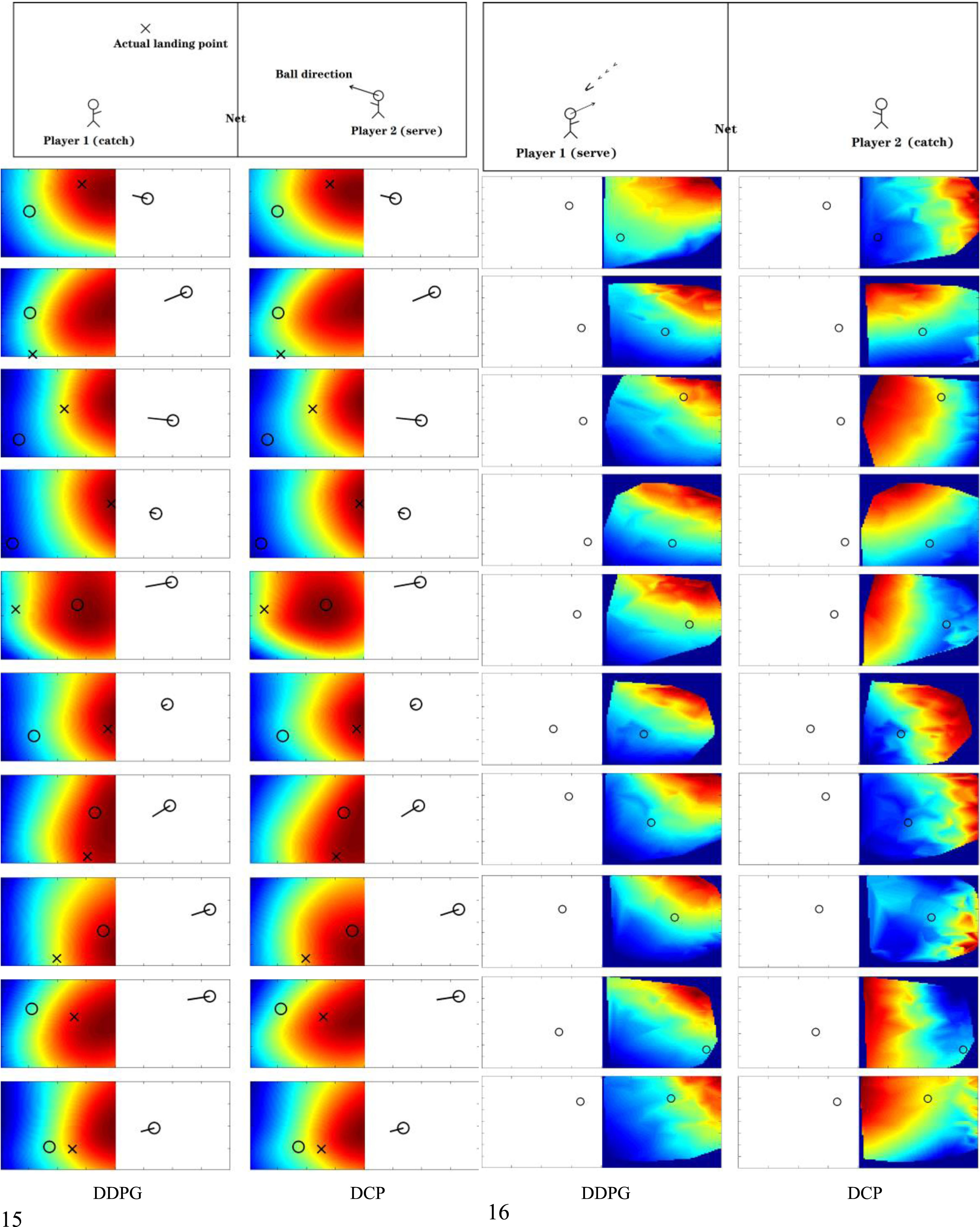
(left). Action-value function learned by the “catch” agent. The hot areas indicate the best locations to capture the ball, comparing DDPG and DCP. Fig. 16(right). Action-value function learned by the “serve” agent. The hot areas indicate the best location to serve the ball to, where the other player is unlikely to capture the ball, comparing DDPG and DCP.

Table 5

Ball catching test of the “catch” agent

Success rate of ball catching
Player 1 (catch)	Player 2 (serve)
	DDPG	DCP (T = 16)	PPO
DDPG	93.2%	90.5%	95.9%
DCP (T = 16)	95.0%	85.8%	95.9%
PPO	81.7%	75.0%	85.2%

(Total 1,000 tests).

4.2.3 DCP can serve skillful balls

We test the performance of the “serve” agent by the error rate defined by Equation (24), only dead ball is considered. Ball captured by the other player or touching within field is not regarded as a fault.

$\begin{matrix} Error rate = \\ \frac{Outside + Hit net}{Outside + Hit net + Captured + Not captured} \end{matrix}$ (24)

Similar to the “catch test”, we visualize the action-value function of the “serve” agent, shown in Fig. 16. A player is serving a ball which has just been captured, in different conditions of players locations. The hot areas indicate the best location to serve the ball to, where the other player is unlikely to capture the ball. We find in some conditions, DDPG and DCP could make different decisions. The difference in action-value function leads to preferences of DDPG and DCP players in behavior stage. For examples, the DCP player in Fig. 8 (left) often serve deep-clear balls, the DDPG player in Fig. 8 (right) often serve smash balls. These preferences happen in both DDPG and DCP players and may result from parameters Initialization. Table 6 lists out the error rate of DDPG players, DCP players and PPO players, respectively. The DCP has the smallest error rate, which is 10% lower than DDPG. Compared with the “catch test”, the “serve test” shows larger difference between DDPG and DCP.

Table 6

Ball serving test of the “serve” agent

Error rate of ball serving
Player 1 (serve)	Player 2 (catch)
	DDPG	DCP (T = 16)	PPO
DDPG	38.6%	41.3%	36.4%
DCP (T = 16)	29.1%	42.1%	23.5%
PPO	40.4%	44.5%	33.8%

(Total 1,000 tests).

4.2.4 The “reset” agent helps to improve ball catching

Since the “reset” agent works a supplementary “catch” agent, we test its performance by a contrast “catch test”: to estimate the success rate of “catch” between enabling the “reset” agent and disabling the “reset” agent. Table 7 shows the incremental success rate as the result from enabling the “reset” agent. A roughly 10% improvement occurs on all DDPG and DCP players. However, the improvement is basically equal, the “reset” agent is not the primary factor for the score difference between the DDPG and DCP teams.

Table 7
Ball catching test of the “catch” and the “reset” agent

Incremental success rate of catching improved by the

“reset network”

Player 1 Player 2 (catch)

(serve) DDPG DCP (T = 16) PPO

DDPG +8.14% +9.13% +2.78%

DCP (T = 16) +9.05% +6.32% +5.46%

PPO +1.27% +0.97% +1.57%

Incremental success rate of catching improved by the
DDPG	+8.14%	+9.13%	+2.78%
DCP (T = 16)	+9.05%	+6.32%	+5.46%
PPO	+1.27%	+0.97%	+1.57%

(Total 1,000 tests).

5 Conclusion

As DDPG is implemented to real-world applications, we find some limitations of DDPG in solving practical problems. The influence of limited action space margin is less discussed in DDPG, which would undermine the training mechanism facilitated by action space margin. Besides, the robustness of DDPG cannot be guaranteed when the random exploration process is large. In this paper, we modified DDPG to DCP by modifying the core updating process of the actor network (policy network): the training is regulated by a T-fold compare among random proposed adjacent actions rather than the partial derivatives from the input layer of the critic network (Q-value network). In comparison, DCP can better deal with applications with complex, dynamic and unknown hard margins in action space. The performance of the first experiment demonstrates that, the accuracy of DDPG is decreased after we adding barrier walls in the path planning task (Fig. 6), while the accuracy of DCP is not influenced by the barrier walls. Besides, the DCP also has an improved robustness in large random process (Table 3) and various reward functions (Table 2). To validate in complex applications, in the second experiment we use a badminton game to examine the collaborative performance of DCP. The total scores show that DCP is able to surpass the DDPG when T is larger than 4 (Table 4) (Fig. 14). To find out the difference, we estimate the individual performance of the three subsystem: the “catch” agent, the “serve” agent and the “reset” agent. Both DDPG and DCP can learn a similar action-value function in ball catching (Fig. 15), but the success rate of DCP is slightly higher (Table 5), though reinforced by the “reset” agent (Table 7). The main difference occurs on the “serve” agent, the action-value functions of ball serving can be different in DDPG and DCP (Fig. 16). Meanwhile, DCP has the lowest error rate in ball serving (Table 6).

Overall, DCP has an obvious improvement from DDPG, and we believe it is effective, efficient and qualified for all DDPG applications. Limited by the paper length, our demonstration may not cover every details and there could be more case studies about DCP. In the future work, we will validate DCP and DDPG to various tasks to obtain a more universal and practical DRL framework.

Data availability

Data and programs in this study are available from the corresponding author upon reasonable request.

Conflicts of interest

All authors declare no conflict of interest.

Funding statement

This study was funded by National Natural Science Foundation of China (grant number 12172287).

Footnotes

Acknowledgments

The authors would like to show gratitude to our colleague, Dr. Zhongyun Fan for providing technical assistance.

References

Sutton

R.S.

and Barto

A.G.

, Reinforcement learning: An introduction. MIT press, 2018, pp. 15–135.

Sutton

R.S.

and Barto

A.G.

, Introduction to reinforcement learning. Cambridge: MIT press, 1998, pp. 25–75.

Pinto

, Davidson

, Sukthankar

, et al., Robust adversarial reinforcement learning, International Conference on Machine Learning. PMLR, (2017), 2817–2826.

Lillicrap

T.P.

, Hunt

J.J.

, Pritzel

, et al., Continuous control with deep reinforcement learning, arXiv preprint arXiv:1509.02971, 2015.

Duan

, Chen

, Houthooft

, et al., Benchmarking deep reinforcement learning for continuous control, International Conference on Machine Learning. PMLR, (2016), 1329–1338.

Silver

, Huang

, Maddison

C.J.

, et al., Mastering the game of Go with deep neural networks and tree search, Nature 529(7587) (2016), 484–489.

Silver

, Schrittwieser

, Simonyan

, et al., Mastering the game of go without human knowledge, Nature 550(7676) (2017), 354–359.

Wei

C.Y.

, Hong

Y.T.

and Lu

C.J.

, Online reinforcement learning in stochastic games. arXiv preprint arXiv:1712.00579, 2017.

Brown

and Sandholm

, Safe and nested subgame solving for imperfect-information games, arXiv preprint arXiv:1705.02955, 2017.

10.

, Xia

, Qin

, et al., Dual learning for machine translation, Advances in neural Information Processing Systems 29 (2016), 820–828.

11.

Williams

J.D.

, Asadi

and Zweig

, Hybrid code networks: practical and efficient end-to-end dialog control with supervised and reinforcement learning, arXiv preprint arXiv:1702.03274, 2017.

12.

Dhingra

, Li

, et al., Towards end-to-end reinforcement learning of dialogue agents for information access, arXiv preprint arXiv:1609.00777, 2016.

13.

, Monroe

, Ritter

, et al., Deep reinforcement learning for dialogue generation, arXiv preprint arXiv:1606.01541, 2016.

14.

Tang

, Reinforcement mechanism design, IJCAI (2017), 5146–5150.

15.

Van

H.H.

, Guez

and Silver

, Deep reinforcement learning with double q-learning, Proceedings of the AAAI Conference on Artificial Intelligence 30(1) (2016).

16.

Zhang

and Yu

, AlphaZero, Deep Reinforcement Learnings. Springer, Singapore, (2020), 391–415.

17.

Oladayo

and Rammohan

, Adaptive evolution strategy with ensemble of mutations for Reinforcement Learning, Knowledge-Based Systems (2022), 108624.

18.

Schulman

, Wolski

, Dhariwal

, et al., Proximal policy optimization algorithms, arXiv preprint arXiv:1707.06347, 2017.

19.

Babaeizadeh

, Frosio

, Tyree

, et al., Reinforcement learning through asynchronous advantage actor-critic on a gpu, arXiv preprint arXiv:1611.06256, 2016.

20.

Wang

, Schaul

, Hessel

, et al., Dueling network architectures for deep reinforcement learning, International Conference on Machine Learning. PMLR, (2016), 1995–2003.

21.

Fortunato

, Azar

M.G.

, Piot

, et al., Noisy networks for exploration, arXiv preprint arXiv:1706.10295, 2017.

22.

Bellemare

M.G.

, Dabney

and Munos

, A distributional perspective on reinforcement learning, International Conference on Machine Learning. PMLR,(2017), 449–458.

23.

Hessel

, Modayil

, Van

H.H.

, et al., Rainbow: Combining improvements in deep reinforcement learning, Proceedings of the AAAI Conference on Artificial Intelligence 32(1), 2018.

24.

Silver

, Lever

, Heess

, et al., Deterministic policy gradient algorithms, International conference on machine learning PMLR (2014), 387–395.

25.

Antonietti

, Casellato

, D’Angleo

, et al., Bioinspired Adaptive Spiking Neural Network to ControlNAORobot in a Pavlovian ConditioningTask, 2018 7th IEEE International Conference on Biomedical Robotics and Biomechatronics (Biorob). IEEE, (2018), pp. 142–147.

26.

Mahadevan

and Connell

, Automatic programming of behavior-based robots using reinforcement learning, Artificial Intelligence 55(2) (1992), pp. 311–365.

27.

Goedhart

, Van

, Armanini

S.F.

, et al., Machine Learning for Flapping Wing Flight Control, 2018 AIAA Information Systems-AIAA Infotech@ Aerospace, 2018.

28.

Verma

and Mettler

, Computational investigation of environment learning in guidance and navigation, Journal of Guidance, Control, and Dynamics 40(2) (2016), pp. 371–389.

29.

and Wang

Y.T.

, Online learning control by association and reinforcement,pp, IEEE Transactions on Neural Networks 12(2) (2001), 264–276.

30.

Kaelbling

L.P.

, Littman

M.L.

and Moore

A W.

, Reinforcement learning: A survey, Journal of Artificial Intelligence Research 4 (1996), pp. 237–285.

31.

Waslander

S.L.

, Hoffmann

G.M.

, Jang

J.S.

, et al., Multi-agent quadrotor testbed control design: Integral sliding mode vs. reinforcement learning, Intelligent Robots and Systems (2005), pp. 3712–3717.

32.

Kim

B.S.

and Calise

A.J.

, Nonlinear flight control using neural networks, Journal of Guidance, Control, and Dynamics 20(1) (1997), 26–33.

33.

Richards

and Boyle

, Combining planning and learning for autonomous vehicle navigation, AIAA Guidance, Navigation, and Control Conference. 2010.

34.

Haldar

, Abdool

, Ramanathan

, et al., Applying deep learning to Airbnb search, Proceedings of the 25th ACM SIGKDD International Conference on Knowledge Discovery & Data Mining (2019), 1927–1935.

Agents	Hidden layers×layer length
	2×32	4×48	6×64
DDPG	85%	89%	90%
DCP	91%	95%	95%
PPO	90%	93%	94%
DQN	88%	91%	90%

Agents	Reward function
	GR	GR+LR	LR
DDPG	89%	82%	71%
DCP	95%	95%	93%
PPO	93%	94%	95%
DQN	91%	90%	87%

Agents	Random process
	σ² = 0.2	σ² = 0.5	σ² = 1.0
DDPG	0%	33%	96%
DCP	0%	0%	0%

Incremental success rate of catching improved by the
“reset network”
Player 1	Player 2 (catch)
(serve)	DDPG	DCP (T = 16)	PPO
DDPG	+8.14%	+9.13%	+2.78%
DCP (T = 16)	+9.05%	+6.32%	+5.46%
PPO	+1.27%	+0.97%	+1.57%

An efficient and robust gradient reinforcement learning: Deep comparative policy

Abstract

Keywords

1 Introduction

2 Methods

2.1 Deep deterministic policy gradient (DDPG)

3.1 Experimental configurations

3.1.1 Task environment

3.2.1 The accuracy of DCP is less influenced by the margins

Table 1 Success rate of the DRL agents (using different network sizes) Agents Hidden layers×layer length 2×32 4×48 6×64 DDPG 85% 89% 90% DCP 91% 95% 95% PPO 90% 93% 94% DQN 88% 91% 90%

Table 2 Success rate of the DRL agents (using different reward functions) Agents Reward function GR GR+LR LR DDPG 89% 82% 71% DCP 95% 95% 93% PPO 93% 94% 95% DQN 91% 90% 87%

Table 3 Rate of training failure (using large random) Agents Random process σ2 = 0.2 σ2 = 0.5 σ2 = 1.0 DDPG 0% 33% 96% DCP 0% 0% 0%

4.1 Experimental configurations

4.1.1 Game environment

4.1.2 Multi-agent collaboration

4.2.1 Overall scores of DCP increase as T increases

Table 4 Overall scores of the three teams

Table 7 Ball catching test of the “catch” and the “reset” agent Incremental success rate of catching improved by the “reset network” Player 1 Player 2 (catch) (serve) DDPG DCP (T = 16) PPO DDPG +8.14% +9.13% +2.78% DCP (T = 16) +9.05% +6.32% +5.46% PPO +1.27% +0.97% +1.57%

Data availability

Conflicts of interest

Funding statement

Footnotes

Acknowledgments

References

Table 1
Success rate of the DRL agents (using different network sizes)

Agents Hidden layers×layer length

2×32 4×48 6×64

DDPG 85% 89% 90%

DCP 91% 95% 95%

PPO 90% 93% 94%

DQN 88% 91% 90%

Table 2
Success rate of the DRL agents (using different reward functions)

Agents Reward function

GR GR+LR LR

DDPG 89% 82% 71%

DCP 95% 95% 93%

PPO 93% 94% 95%

DQN 91% 90% 87%

Table 3
Rate of training failure (using large random)

Agents Random process

σ² = 0.2 σ² = 0.5 σ² = 1.0

DDPG 0% 33% 96%

DCP 0% 0% 0%

Table 4
Overall scores of the three teams

Table 7
Ball catching test of the “catch” and the “reset” agent

Incremental success rate of catching improved by the

“reset network”

Player 1 Player 2 (catch)

(serve) DDPG DCP (T = 16) PPO

DDPG +8.14% +9.13% +2.78%

DCP (T = 16) +9.05% +6.32% +5.46%

PPO +1.27% +0.97% +1.57%