Multidimensional clustering analysis of mathematical knowledge difficulty based on Gspan

Abstract

In addition to providing learners with a large amount of teaching resources, online teaching platforms can also provide learning resources and channels such as video courseware, Q&A tutoring groups, and forums. However, currently, there are still shortcomings in depth and dimensionality in mining student learning behavior data on the platform. In view of this situation, based on the learning interaction behavior, this study established the difficulty similarity model of knowledge points, and used spectral clustering to classify their difficulty. In addition, the study intended to use the maximum frequent subgraph under the Gspan framework to characterize learners’ implicit learning patterns. The outcomes expressed that the algorithm put forward in the study achieved the highest accuracy index of 98.8%, which was 1.4%, 4.0%, and 8.6% higher than Apriori-based graph mining algorithms, K-means, and frequent subgraph discovery algorithms. In terms of F1 index, the convergence value of the algorithm proposed in the study was 95.5%, which was about 2.5% higher than the last three algorithms. In addition, learners of all three cognitive levels had the highest maximum number of frequent subgraphs with sizes above 100 when the minSup value was 60%. And when the number of clusters was 3, the clustering accuracy of the three learners was the highest. In similarity calculation, the calculation method used in the study was at the minimum in terms of root mean square error and absolute error average index, which were 0.048% and 0.01% respectively. This indicated that the model proposed by the research had better classification effect on the difficulty of knowledge points for learners of different cognitive levels, and had certain application potential.

Keywords

1 Introduction

At present, China’s education is in a critical transition period from winning by quantity to quality. It is a major issue that higher education in China currently faces, as it can ensure the continuous increase in the number of educated individuals and steadily improve the quality of education [1]. The development of Internet and computer multimedia technologies has promoted the networking and internationalization of education and the integration of “Internet plus education” [2]. In this context, various online teaching platforms have emerged and developed rapidly. This learning method breaks the limitations of time and space, allowing more students to access high-quality teaching resources and achieving optimal allocation of teaching resources. In addition to providing learners with a large amount of teaching resources, online teaching platforms can also provide them with learning resources and methods such as video courseware, Q & A tutoring groups, and forums. On online teaching platforms, multidimensional interactive information and evaluation results generated by students will be automatically saved. Using data mining and learning analysis techniques, it explores the implicit learning characteristics of learners from their interactive behavior data [3]. It finds the correlation between learners’ interactive behaviors and learning effects, analyzes the internal links between learners’ various behaviors, and comprehensively understands learners’ learning conditions, which is helpful to guide learners’ active learning, to improve the effect of learners’ online learning [4]. This has important guiding significance for guiding teachers in timely classroom teaching, promoting the shift of classroom teaching mode towards knowledge construction, and establishing the best classroom elements and teaching methods. Because teachers and learners are spatially separated, students cannot promptly ask teachers when facing learning issues. Teachers are also unable to monitor students’ learning in real-time, so they are unable to timely grasp their learning status during the learning, and thus cannot objectively evaluate their learning outcomes. Although teachers can evaluate the difficulty of knowledge points (KPs) through their own teaching experience, there are significant difficulties for students with different levels of knowledge. The conventional educational methods include questionnaires, inquiries, and interviews to understand students’ learning status. However, this method not only consumes a huge amount of time, but also is influenced by students’ subjective emotions, resulting in shortcomings in accuracy and realism, making it difficult to reflect the true KPs in the course. Utilizing multidimensional interactive data in online learning platforms, mining learners’ implicit learning features and patterns, researching knowledge difficulty classification algorithms, and accurately classifying knowledge difficulty for learners of different cognitive levels can help teachers understand learners’ knowledge difficulties in a timely manner and continuously optimize the design of adaptive teaching content. Thus, it can better implement individualized teaching to assist teachers in timely understanding the knowledge difficulties encountered by students during learning and determine the teaching priorities and difficulties in the classroom and improve classroom efficiency. In view of this, this study proposes a knowledge difficulty clustering algorithm based on multidimensional temporal data (MTD). From the similarity calculation of KP difficulty, learning path network, maximum frequent subgraph based on learning path, spectral clustering (SC) and other aspects, a better knowledge difficulty classification model is developed.

This study is mainly composed of the following four parts. The second part is a literature review on multidimensional clustering analysis (MCA) and the Gspan algorithm. The third part is the construction of a knowledge difficulty point classification model. The fourth part is the utility validation of the proposed clustering model based on different datasets. Finally, a summary of the research methods and results is provided. The contribution of this study is to address the limitations of existing KP difficulty clustering algorithms in multi-dimensional interactive behavior clustering. A KP difficulty clustering algorithm based on multidimensional time series data and maximum frequent subgraphs is proposed, and a knowledge points difficulty similarity (KPDS) measurement model is constructed to calculate the KP difficulty similarity matrix. Based on the obtained similarity matrix, SC algorithm is used to achieve KP difficulty classification. The innovation of the research lies in proposing a knowledge difficulty clustering algorithm based on MTD and maximum frequent subgraphs. This algorithm extracts the maximum frequent subgraph from the directed learning path graph set of learners using the Gspan-based maximum frequent subgraph mining algorithm, and combines the degree of system interaction and the maximum frequent subgraph to characterize the difficulty similarity of KPDS based on system interaction behavior.

2 Related Works

Many scholars have conducted detailed research on MCA. In terms of enterprise clustering analysis, Scholars such as Ljungkvist and Andersén proposed a multidimensional classification method for “ecological entrepreneurs” in small manufacturing enterprises. Based on cluster analysis of 312 Swedish enterprises, four different clusters could be identified: pioneer, green waste, regulatory and recycling enterprises. These clusters compared their entrepreneurial direction and corporate performance level [5]. Clustering on diverse datasets, Ventocilla and Riveiro presented an empirical user study comparing eight multidimensional projection techniques to support the estimation of the amount of clusters k embedded in six multidimensional datasets. The choice of technology was based on the expected design or usage structure of its visual encoded data, that is, the neighborhood relationship between data points or groups of data points in the dataset [6]. Park and other research teams proposed a new multi-view SC frame work to integrate different types of omics data measured from the same subject. It learned the weights of each data type and measured the similarity between patients through a non convex optimization framework. The ADMM algorithm was used to iteratively solve this non-convex problem and its convergence was proved. The accuracy and robustness of the method have been assessed theoretically and through various synthetic data [7]. In the construction of evaluation and statistical models, Cerquetti and Cutrini proposed a multidimensional approach to measure and evaluate the resilience of museums as a whole. This study emphasized the lack of a framework to understand the resilience level of museums and their contribution to resilience. The results indicated that human resources were a common area that needed improvement [8]. Little et al. provided a theoretical framework for analyzing the quality of embedded samples generated by classical multidimensional scaling. This laid the foundation for various downstream statistical analyses, focusing on clustering noise data. The findings provided a scaling condition for signal-to-noise ratio, under which classic multidimensional scaling and distance based clustering algorithms could restore the clustering labels of all samples. Simulation research have evidenced that these scaling conditions were sharp [9]. Fradi and Samir introduced a statistical model for clustering functions and populations of multidimensional curves defined as real number intervals, and explored Bayesian models with spherical Gaussian process priors using statistical geometry in a smooth density space. Finally, the practical significance of the method was demonstrated [10]. Scholars such as Vera and Macías analyzed clustering on equivalent partition configurations related to full dimensional scaling and appropriate conversion to square differences. A Monte Carlo experiment was conducted to contrast the outcomes gained by the tested method with those obtained by programs directly applicable to dissimilarity matrices [11].

Many scholars have conducted extensive research on the Gspan algorithm. In terms of intelligent biological feature mining and emotion recognition, Al Janabi and Salman proposed a smart data analysis model to identify the optimal patterns of human activity. This model generated patterns from the optimal subgraph using an association pattern algorithm called Gspan [12]. Hassan and Mohammed used Gspan frequent subgraph mining algorithm to find frequent Substructure in the graph database of each emotion. Different research was conducted using Surrey’s audiovisual emotional expression database, and the final system accuracy was 90.00%. The experimental outcomes denoted that the accuracy of the system had significantly improved [13]. Kadhuim Al-Janabi and other scholars have established a new intelligent deep analysis algorithm, which first converted DNA sequences into RNA sequences, and then divided these sequences into multiple sub sequences through specific equations that determine the starting and ending points of each sequence. The findings indicated that the algorithm had better robustness [14]. In computer resource calculation or abnormal data filtering, the research team of Bilgin and Murat solved the high memory consumption based on frequent subgraph mining and proposed a new method called predictive dynamic size structure encapsulation to minimize the memory requirements of the FSM algorithm [15]. Liu and Zhou proposed a Gspan-based digital distribution device anomaly data screening method to improve the accuracy and efficiency of anomaly data screening and reduce data loss rate. The research outcomes demonstrated that the minimum data screening time of this method was 6.2 seconds, and the screening error was always below 0.2 [16]. Cekinel and Karagoz constructed a graph representation of news articles and proposed a pattern extraction method based on graph mining. The raised method was analyzed relative to the baseline method on news sets and benchmark news datasets from online newspapers [17].

In summary, in MCA, scholars mainly focus on diversified data such as enterprise management and visual projection spectral data, as well as constructing practical evaluation models based on multidimensional clustering. In terms of the use of the Gspan algorithm, scholars have mainly conducted research on data filtering and analysis in the fields of biology and emotion mining. Fewer scholars have applied it in education. In view of this, this study aims to propose a KP difficulty clustering algorithm based on MCA and Gspan to explore students’ learning situation.

3 KP Difficulty Clustering Algorithm Based on MTD and Gspan

To better assist teachers in timely understanding the knowledge difficulties encountered by students during learning and better determine the teaching priorities and difficulties in the classroom and improve classroom efficiency, this study proposes a maximum frequent subgraph mining algorithm based on MTD and Gspan. The algorithm depicts the degree of interaction among learners, describes the KPDS based on an improved similarity model, and represents the learning patterns of learners learning different difficulty KPs based on the maximum frequent subgraph [18].

3.1 Knowledge difficulty clustering algorithm based on MTD

It needs to quantify the three types of interaction behaviors of learners to obtain corresponding learner KP interaction degree matrices, and prepare for the subsequent calculation of KPDS. There are three types of learning interaction, namely system interaction, teacher-student interaction, and student interaction. Among them, the system interaction refers to the degree of learning engagement of learners when learning KP videos online, and the online learning platform stores the learning behavior records of learners watching each KP video. The teacher-student interaction refers to the degree of learning engagement between learners and teachers. By analyzing the Q&A text data between teachers and students, the frequency and effective duration of interaction between teachers and students regarding KPs can be extracted. The interaction between students refers to the degree of learning engagement between learners and other learners. By analyzing the text data of students discussing KPs with other classmates, the frequency and effective interaction duration of KPs can be extracted. The level of interaction means the degree to which students participate in the learning process during online learning. The online learning platform stores the learning behavior records of students who watch videos of various KPs [19]. By extracting behavioral features from the learning activity log, the interaction level between learner u and KP i can be described, as expressed in Formula (1). ${SC}_{u, i} = λ_{1} \times f_{{SC}_{u, i}} + λ_{2} \times t_{{SC}_{u, i}} + λ_{3} \times p_{{SC}_{u, j}}$ (1)

In Formula (1), f_{SC
_u,i} refers to the frequency at which students learn KPs. t_{SC
_u,i} indicates the length of time for learners to learn KPs. p_{SC
_u,j} means the pause frequency and fast forward frequency of students in the process of learning point process of knowledge. λ₁, λ₂, and λ₃ express weight coefficients. Figure 1 is a schematic diagram of the knowledge difficulty clustering algorithm based on MTD.

Fig. 1

Schematic diagram of knowledge difficulty clustering algorithm based on MTD.

From Fig. 1, by analyzing learners’ interactive behavior, an interaction level matrix and a directed learning path network for the group can be obtained. Analyzing that can obtain the centrality of KP entry, and inputting the centrality of KP entry and interaction degree matrix into the KPDS model based on interaction behavior will obtain the KPDS matrix. According to the similarity matrix, the SC method is applied to the classification of difficult points, and the amount of KPs is k. Teachers can determine the difficulty of each class through relevant knowledge clusters. Figure 2 shows a bipartite graph of KPs and learners.

Fig. 2

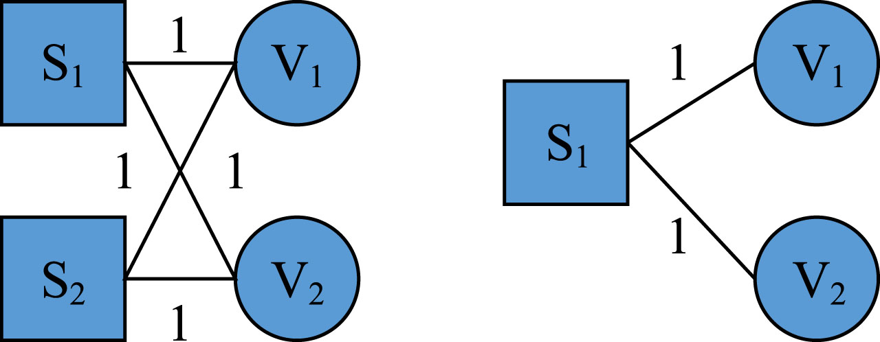
KPs and learners’ bipartite graphs.

S₁ and S₂ stand for learner 1 and learner 2, respectively; V₁ means KP 1, and the associated edges of S₁ and V₁ denote that learner 1 has learned KP 1 once. Formula (2) is used to calculate the relationship between the degree of interaction and the degree of difficulty in CLN. ${Sim}_{SC}^{proposed} (i, j) = {Sim}_{degree} (i, j) \times {Sim}_{GDLPN} (i, j)$ (2)

In Formula (2), Sim_degree (i, j) indicates the similarity in difficulty of KPs i and j on the ground of the degree of system interaction. Sim_GDLPN (i, j) means the similarity in difficulty of KPs in a group directed learning path network based on KPs i and j. Through the analysis of students’ interactive behavior, it is found that learners tend to complete each KP video, which leads to a small number of interaction matrices for learners. In the case of low sparsity, the improved cosine similarity calculation method is more constant than other similarity evaluation methods. Formula (3) calculates the complexity of KPs based on two levels of interaction. $\begin{matrix} {Sim}_{degree} (i, j) = \\ \frac{\sum_{u \in {KP}_{i}^{SC} \cap {KP}_{j}^{SC}} ({SC}_{u, i} - {\bar{SC}}_{u}) \times ({SC}_{u, j} - {\bar{SC}}_{u})}{\sqrt{\sum_{u \in {KP}_{i}^{SC} \cap {KP}_{j}^{SC}} {({SC}_{u, i} - {\bar{SC}}_{u})}^{2}} \sqrt{\sum_{u \in {KP}_{i}^{SC} \cap {KP}_{j}^{SC}} {({SC}_{u, j} - {\bar{SC}}_{u})}^{2}}} \end{matrix}$ (3)

In Formula (3), SC_u,i indicates the level of systematic interaction between learner u and KP i. ${\bar{SC}}_{u}$ means the average system interaction level of the learner’s u. ${KP}_{i}^{SC}$ denotes the set of learners who have interacted with KPs i. ${KP}_{j}^{SC}$ represents the set of learners who have interacted with the KP j. Figure 3 shows the structure of some knowledge nodes in a group directed learning path network.

From Fig. 3, in the directed learning path, the degree of entry of nodes represents students’ repeated learning of KPs. The forgetting curve proposed by Ebbinghaus suggests that the interactive behavior of repeated learning may not be related to the difficulty of the KPs, but rather to students’ forgetting. On this basis, the input center of the directed weighted network will be used for quantitative analysis, as shown in Formula (4).

Fig. 3

Partial knowledge node structure in group directed learning path networks.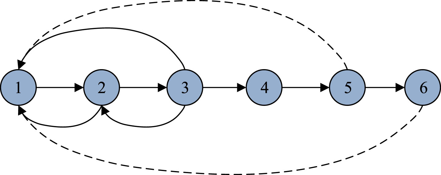

$D_{{in}_{β}} (v_{i}) = k_{v_{i}}^{{in}_{β}} \times {(\frac{s_{v_{i}}^{{in}_{β}}}{k_{v_{i}}^{{in}_{β}}})}^{α}$ (4)

In Formula (4), α means an adjustable parameter used to adjust the number of adjacent entry nodes, thereby controlling the centrality of entry. β denotes the forgetting interval of the sequence of KPs for learners to learn the course. The number of nodes in the β sequence between $k_{v_{i}}^{{in}_{β}}$ and KP v_i, and in the set of directly connected entry nodes of KP v_i. $s_{v_{i}}^{{in}_{β}}$ means the sum of edge weights of nodes within β between the v_i sequence of KPs and in the set of directly connected entry nodes of KP v_i. Formula (5) is the similarity expression for the difficulty of KPs in a group directed learning path network. ${Sim}_{GDLPN} (i, j) = \frac{1}{1 + | D_{{in}_{β}} (v_{i}) - D_{{in}_{β}} (v_{j}) |}$ (5)

In Formula (5), D_{in
_β} (v_i) denotes the centrality of the KP i. D_{in
_β} (v_j) indicates the centrality of the KP j. The closer the D_{in
_β} of two KPs, the more similar the difficulty of the two KPs. In the actual teaching process, teachers should determine the number of difficulty clusters K of KPs with the specific teaching content and teaching design, and then use SC algorithm to classify the difficulty of KPs of the course based on the difficulty similarity matrix of the KPs obtained. It assumes that there are n KPs, and they are divided into K categories. Based on this, a SC algorithm for different KPs is established. Among them, the KPDS matrix is established through M = [M_i,j] _n×n, and according to Formula (6), the M is constructed with Laplacian matrix L. $L = D^{- 1 / 2} (D - M) D^{- 1 / 2}$ (6)

In Formula (6), D belongs to the diagonal matrix. The eigenvalues of Laplacian matrix L are solved, the corresponding K eigenvalues are extracted in descending order, the feature subspace F of N * K dimension is constructed, and the feature subspace is classified by K-means method to achieve the classification of K samples.

3.2 Maximum frequent subgraph mining algorithm based on Gspan

It provides a set of labeled graphs D ={ G₁, G₂, . . . , G_n } and a threshold minSup for maximum frequency. If a subgraph g is a frequent subgraph and the hypergraph of that subgraph in the label graph set is not a frequent subgraph, then the subgraph is defined as the maximum frequent subgraph. The given tag set D is shown in Fig. 4.

Fig. 4

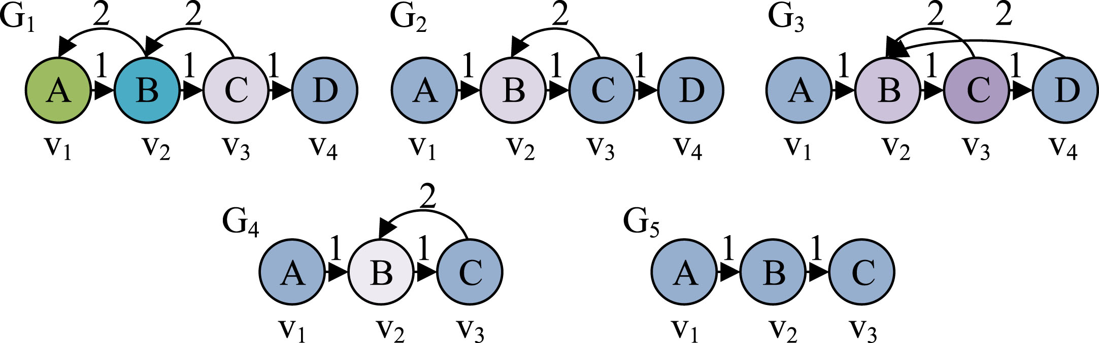
Sample tag atlas.

The number of frequent subgraphs extracted is enormous. For labeled graphs with n frequent edges, the number of frequent subgraphs can reach 2n. Moreover, the number of frequent subgraphs often increases exponentially with their size, making analysis of frequent subgraphs difficult. The maximum frequent subgraph is composed of multiple subgraphs, which not only ensures the integrity of subgraphs but also reduces the frequency of subgraphs appearing. Therefore, this study will select the maximum frequency subgraph for analysis. MAGIN and SPIN are classic algorithms for mining maximum frequent subgraphs. Both methods are based on the principle of extracting all frequent subgraphs and then extending the frequent subgraphs to the maximum frequency subgraph. Considering the direction and cyclic characteristics of the network, the Gspan method is studied to extract all frequent subgraphs. Figure 5 shows the strategy flowchart of the Gspan algorithm.

Fig. 5

Strategy flowchart of Gspan algorithm.

From Fig. 5, by traversing the entire image set, the frequency of all points and edges present in all the images will be obtained. Then, it inserts each individual frequent edge into the frequent subgraph and expands them into the first frequent itemset. It adds edges to frequent subgraphs of order k, and then extends them to candidate subgraphs of order k + 1. It calculates support for K-rank+1 and removes subgraphs that do not meet the minimum support. It performs DFS encoding on candidate subsets that meet the support threshold, verifies that their DFS encoding is min-DFS, removes non candidate subsets, and places the remaining candidate subgraphs into frequent subgraphs until all frequent subgraphs are extracted from the entire image set without further increase in frequency subgraphs. Finally, it returns the frequent subgraphs required by the Gspan algorithm. Formula (7) is the support calculation formula in the Gspan algorithm. $SUP (s) = \frac{| {G | s \subset G, G \in GD} |}{| {G^{'} | G^{'} \in GD} |}$ (7)

In Formula (7), | { G|s ⊂ G, G ∈ GD } | denotes how many graphs in the graph set GD are supersets of s. | { G′|G′ ∈ GD } | represents how many graphs are in the graph set GD. So this formula represents the proportion of the graph containing s in the entire graph set. Figure 6 shows the storage structure of the Gspan algorithm.

Fig. 6

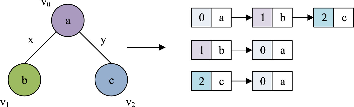
The storage structure of Gspan algorithm.

The memory architecture of Gspan is an adjacent linked list, where the number of vertices in each graph determines how many adjacent links each graph requires. Due to the research involving directional maps, they were not saved twice in the memory of adjacent linked lists. It uses Gspan to mine all frequent subgraphs and maintain the maximum list of frequent subgraphs during the mining process. If it is a frequent subgraph, it needs to be verified that it has the same relationship as the candidate graph in the maximum frequency subgraph. If one graph is isomorphic to another graph, it needs to remove it from the list and add it to the largest graph. Formula (8) is an expression for calculating the KPDS based on the maximum frequent subgraph.

$\begin{matrix} {Sim}_{struct} (i, j) = \\ \frac{1}{1 + | \frac{\sum_{s_{l}^{max} \in S (v_{i})} Sup (s_{l}^{max}, GD)}{S (v_{i})} - \frac{\sum_{s_{l}^{max} \in S (v_{j})} Sup (s_{l}^{max}, GD)}{S (v_{j})} |} \end{matrix}$ (8)

In Formula (8), S (v_i) means the maximum frequent subgraph set containing knowledge node i. S (v_j) indicates the maximum frequent subgraph set containing knowledge nodes j. $Sup (s_{l}^{max}, GD)$ represents the support of subgraphs in the graph set GD.

4 Result analysis of KP difficulty clustering algorithm based on MDT and Gspan

To understand learners’ mastery of KPs with different difficulty levels, this study designed a knowledge difficulty clustering algorithm based on MTD and maximum frequent subgraphs. To verify the performance and utility of the algorithm, it would be analyzed from the time and spatial analysis, accuracy, precision and other indicators during the experiment. And it analyzed the application results of this algorithm from the clustering effects of learners with different cognitive levels.

4.1 Performance analysis of Gspan algorithm based on multidimensional cluster analysis

The dataset selected for the study was the commonly used benchmark dataset in text classification tasks, namely the Eurlex and Wiki10 datasets, which were divided into training and testing data samples [20]. The number of training and testing samples for Eurlex data was 15449 and 3865, respectively, with 3956 labels and an average text length of 1230.1. The amount of training and testing samples for the Wiki10 dataset was 14146 and 6616, respectively, with 30938 tags and an average text length of 2425.5. In terms of algorithm performance evaluation indicators, this study selected accuracy, precision, recall, and F-Measure as evaluation indicators to quantitatively analyze the classification performance of different clustering algorithms. Figure 7 expresses the comparison results of the number of GspanMAX and Gspan subgraphs.

Fig. 7

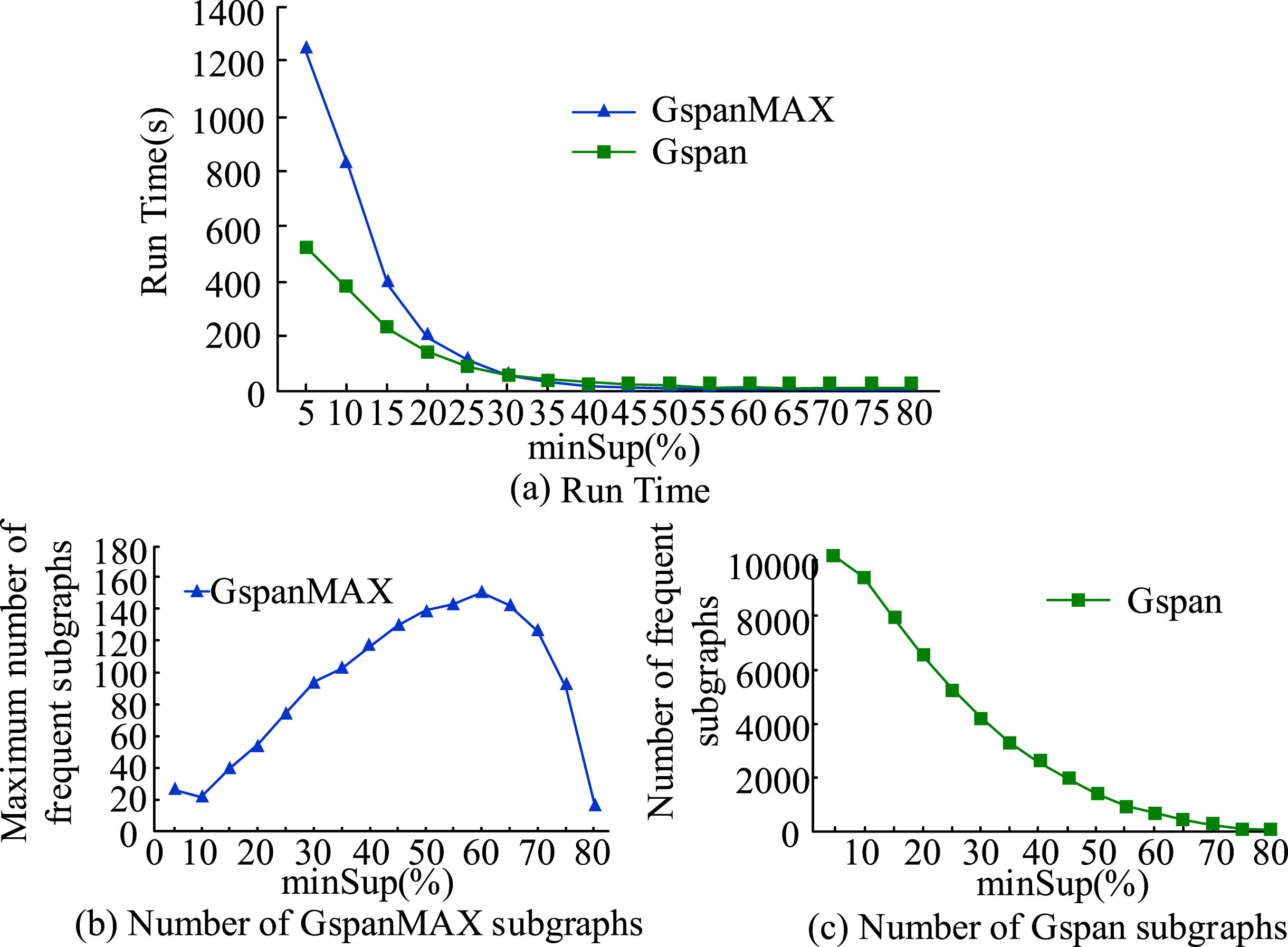
Comparison of the number of GspanMAX and Gspan subgraphs.

From Fig. 7 (a), as minSup increased, the algorithm running time decreased for both Gspan and GspanMAX. When the minSup value was less than 30%, Gspan had a faster computational speed compared to GspanMAX. This was mainly because when the size of minSup is small, GspanMAX had more frequent edges and could discover more frequency subgraphs. Therefore, it was necessary to make multiple judgments on the candidate graph to determine its isomorphism with the graph in the maximum frequency subgraph. When minSup exceeded 30%, the execution time of Gspan and GspanMAX was basically the same. This was mainly because as minSup became higher, the amount of frequently occurring subgraphs became lower, resulting in a lower number of subgraph isomorphism judgments required for GspanMAX. From Figs. 7 (b) and (c), there were many frequent subgraphs in the Gspan algorithm. When minSup = 5%, 10165 subgraphs could be obtained. Frequent subgraphs might make it difficult to analyze learners’ behavior in the future. When minSup = 60%, the maximum number of subgraphs was 148. Fewer subgraphs could be used to analyze learners’ learning patterns in the future. Unlike frequent subgraphs, the maximum number of frequent subgraphs first increased and then decreased with the increase of minSup. This was because extremely frequent subgraphs could be utilized to cover complex situations of frequent subgraphs with a large number of nodes. Although this method could reduce the number of subgraphs, it could not express the difficulty between KPs due to the large number of nodes involved. To describe the difficulty similarity between KPs, it needed to select a rich maximum frequent subgraph. In view of this, this study set the minSup value to 60%, which was the maximum number of frequent subgraphs that the algorithm could mine. Figure 8 shows the spatiotemporal analysis of frequent subgraphs mined by AC-Gspan and Gspan.

Fig. 8

Spatiotemporal analysis of AC Gspan and Gspan mining frequent subgraphs.

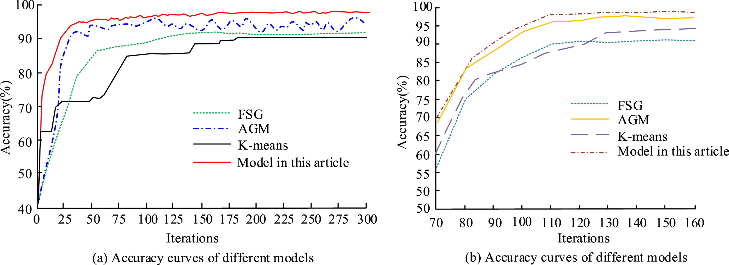
From Fig. 8 (a), as the support parameter increased, the average running time of Gspan and AC-Gspan algorithms showed an overall increasing trend. However, when the support parameter changed between 55 and 100, the average running time of Gspan algorithm was lower than that of AC-Gspan algorithm. When the support parameter was less than or equal to 75, the difference in average running time between the two was not significant, and both remained within 700 ms. However, when the support parameter was higher than 80, the difference in average running time between the two gradually increased, and the maximum difference occurred when the support parameter was 100, with a size of 2980 ms. This was because AC-Gspan has increased the determination of whether subgraphs were closed during the stage, but mining true hypergraphs through closure determination would increase the computational time of the algorithm. From Fig. 8 (b), the memory usage increased with the increase of support parameters in both algorithms. However, the memory usage of the Gspan algorithm was lower than that of the AC-Gspan algorithm under various support parameters. Especially, when the support parameter was greater than or equal to 80, the memory usage of the Gspan algorithm was much lower than that of the AC-Gspan algorithm. When the support parameter was 100, the maximum difference in memory usage between the two was 152MB. Figure 9 shows the comparison curves of the accuracy and accuracy indicators of different algorithms. The comparison algorithms were K-means [21], Apriori-based Graph Mining (AGM) [22], and Frequent subgraph Discovery (FSG) [23].

Fig. 9

Comparison curves of accuracy and accuracy indicators of different algorithms.

Figure 9 (a) shows that the accuracy curve of the K-means had many fluctuating nodes, and the accuracy changed significantly under different iterations. It only showed a horizontal trend after the number of iterations exceeded 180. The numerical difference between FSG and AGM algorithms was significant in the early stage of the experiment, and as the amounts of iterations increased, the maximum difference between the two was greater than 5%. The research proposed that the accuracy of the model was 98.5%, and its overall trend of change was relatively level, and it returned to a stable trend after more than 100 iterations. In Fig. 9 (b), the accuracy changes of the four algorithms were significant. Although the overall trend was on the rise, the proposed model had the highest slope of curve rise, and the maximum value approached 1.0 at 160 iterations, with a size of 98.8%. The accuracy of AGM, K-means, and FSG algorithms at 160 iterations was lower than that of the proposed algorithms, with sizes of 97.4%, 94.8%, and 90.2%, respectively. By comparison, the algorithm proposed by the research institute has improved the accuracy indicators by 1.4%, 4.0%, and 8.6% compared to these three algorithms, respectively. In addition, from the perspective of iterative convergence performance in the middle and later stages of the curve, the proposed model had the smallest curve fluctuation, while the FSG model had the largest fluctuation. Therefore, this indicated that the improved Gspan algorithm used in the study had advantages in classification accuracy and efficiency. Figure 10 shows the result curves of different models on recall and F1 values.

Fig. 10

Comparison of storage modulus fitting results between different models.

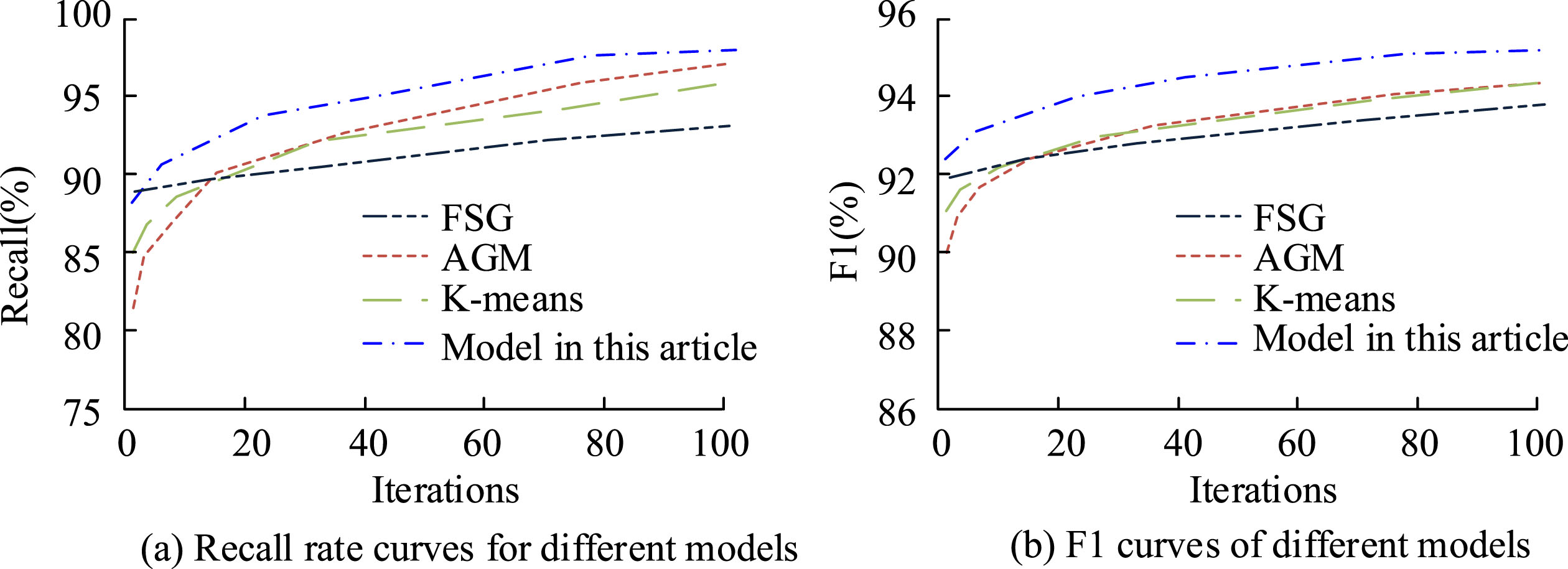
From Fig. 10 (a), the starting value of the recall curve of the model proposed in the study was 87.4%, and the curve rose rapidly. When the iteration times were around 80, the curve began to converge, and the convergence process was stable without any fluctuations. When the iteration times were 100, the convergence value of the recall curve was 97.2%. The recall rates for FSG, AGM, and K-means models with 100 iterations were 92.5%, 93.6%, and 94.7%, respectively. By comparison, the proposed model has increased the recall index by 4.7%, 3.6%, and 2.5% compared to the last three models. From Fig. 10 (b), on the F1 indicator, the model proposed in the study has been at the highest value from the beginning of the iteration to the end of the iteration. Among them, the initial F1 value was 91.8%. When the number of iterations was 79, the curve began to converge, and the F1 value was 95.8%. When the number of iterations was 100, the F1 convergence value of the curve was 95.5%. The F1 values of FSG, AGM, and K-means models were all below 95% when the number of iterations was 100.

4.2 Analysis of the application effect of difficulty clustering based on Gspan KP

To verify the clustering effect of MTD and Gspan algorithm on the difficulty of mathematical KPs, this study selected 216 mathematics course data from a certain online school for analysis. The course included advanced mathematics, linear algebra and probability statistics. Some sample data excerpts are shown in Table 1.

Table 1
Selected partial sample data

Number KP name System interaction Teacher-student Interaction behavior

behavior interaction behavior between students

Interaction duration(s) Interaction frequency Interaction duration(s) Interaction frequency Interaction duration(s) Interaction frequency

1 Multivariable calculus 686 4 203 2 84 1

2 Nth order matrix calculation 734 5 57 1 212 3

3 sequence limit 367 3 142 1 136 3

4 Law of large numbers 497 1 138 2 242 2

5 Ordinary differential equation 348 2 105 4 17 2

Number	KP name	System interaction	Teacher-student	Interaction behavior
1	Multivariable calculus	686	4	203	2	84	1
2	Nth order matrix calculation	734	5	57	1	212	3
3	sequence limit	367	3	142	1	136	3
4	Law of large numbers	497	1	138	2	242	2
5	Ordinary differential equation	348	2	105	4	17	2

Interaction behavior was divided into three types: system, teacher-student and student interactions, and the interaction behavior was recorded according to the interaction duration and frequency. During the experiment, to investigate the impact of different cluster numbers on clustering accuracy, four cluster numbers were set as 2, 3, 4, and 5, respectively. Figure 11 shows the maximum number of frequent subgraphs for learners of different cognitive levels.

From Fig. 11, the max number of frequent subgraphs for learners of three cognitive levels showed a trend of first increasing and then decreasing as the minSup value increases. For learners with intermediate cognitive levels, the growth rate of the maximum number of frequent subgraphs was the fastest, followed by those with elementary cognitive levels, and those with advanced cognitive levels were the slowest. All three types of learners achieved the highest number of frequent subgraphs at a minSup value of 60%, with the order from beginner, intermediate to advanced being 128, 143, and 100. By comparison, learners with intermediate cognitive levels have increased the maximum number of frequent subgraphs by 15 and 43 compared to the other two types of learners. When the minSup value was higher than 60%, the maximum frequent subgraph curve began to decrease. Among them, those with intermediate cognitive levels had the fastest decline in the curve. When minSup was set to 80%, its value dropped to 22, with a decrease of 121. The curve of the maximum number of frequent subgraphs for learners with a cognitive level of beginner and advanced was the second fastest. When minSup was set to 80%, the maximum number of frequent subgraphs was 28 and 27, respectively. Figure 12 shows the clustering accuracy box plot of learning rules at different cognitive levels.

Fig. 11

Maximum number of frequent subgraphs for learners with different cognitive levels.

Fig. 12

Boxplot of clustering accuracy for learning rules at different cognitive levels.

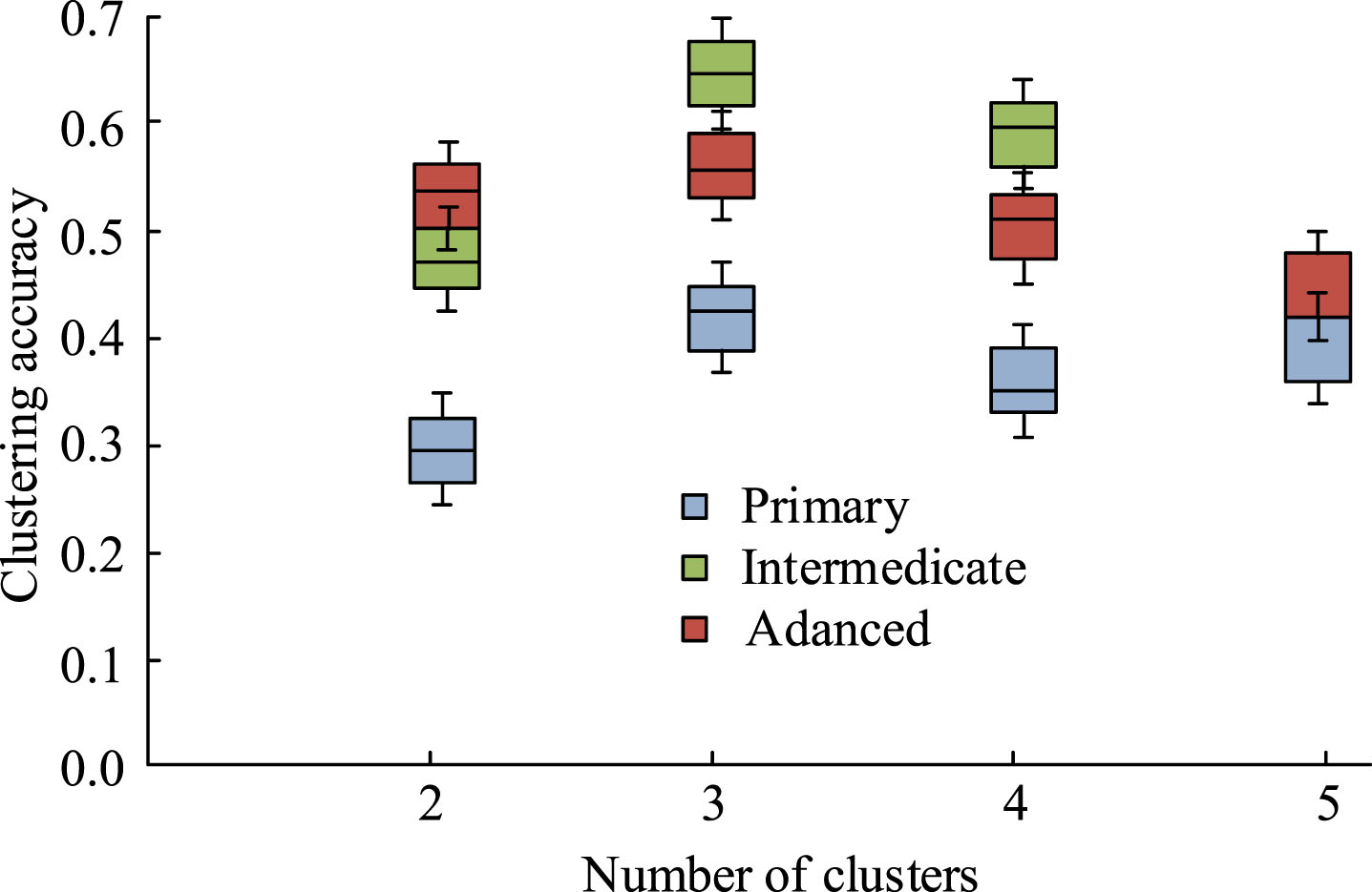
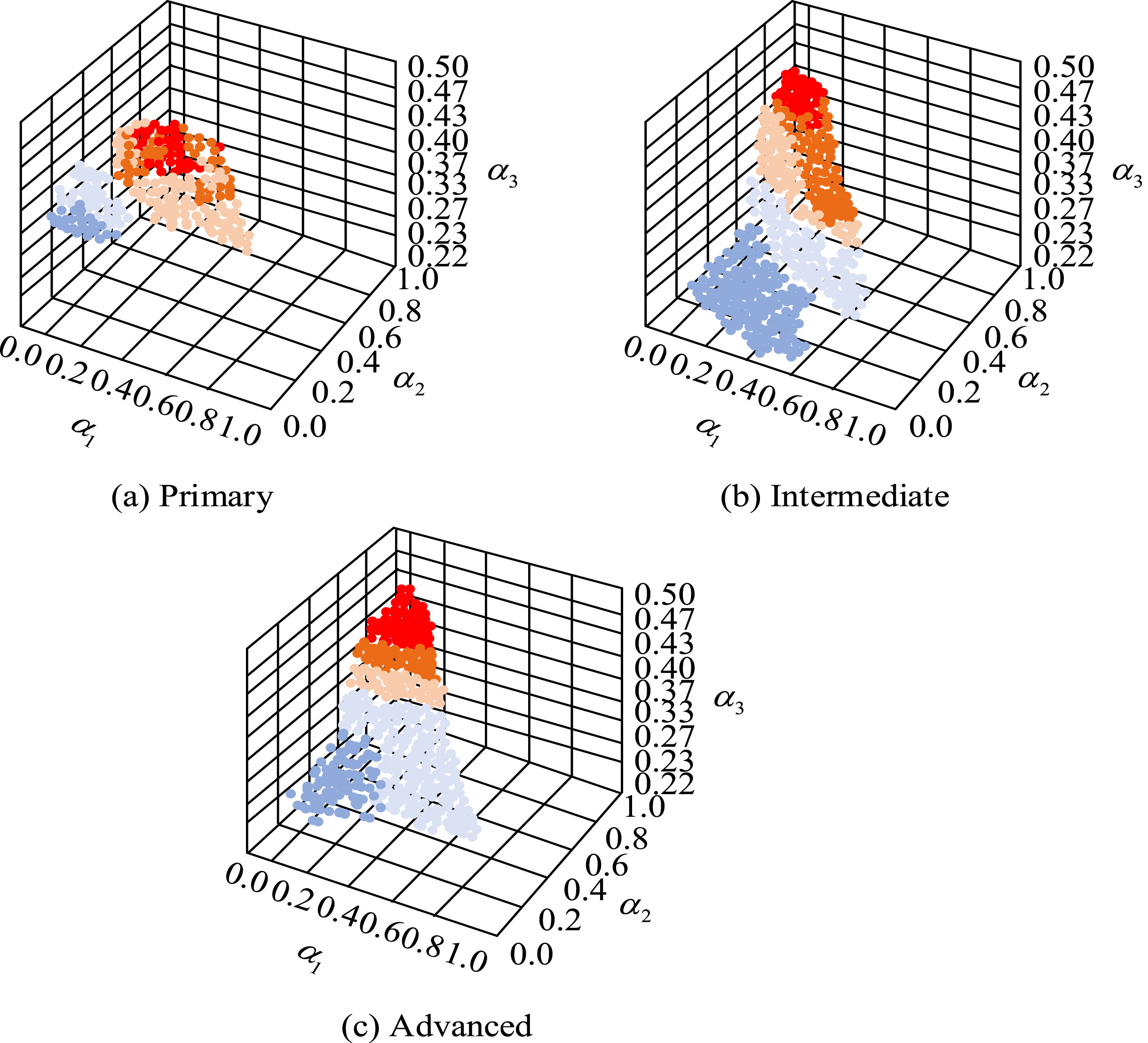
From Fig. 12, different settings for the number of clusters would lead to differences in clustering accuracy. When the clustering accuracy changed between 2 and 5, the clustering accuracy roughly showed a trend of increasing first and then decreasing. When the number of clusters was set to 3, the clustering effect was best for learners of three cognitive levels, with the highest clustering accuracy, ranging from 0.42, 0.64, and 0.56 for primary to advanced clustering. At this point, the algorithm had the best clustering effect for those with intermediate cognitive levels. When the amounts of clusters were around 3, the clustering accuracy decreased to varying degrees. When the amounts of clusters were set to 2, the clustering accuracy from beginner learners to advanced learners was 0.31, 0.48, and 0.52, respectively. At this point, the algorithm had the best clustering effect on individuals with advanced cognitive levels. When the amounts of clusters were set to 4, the clustering accuracy decreased, and the clustering accuracy of beginners to advanced learners was 0.4, 0.44, and 0.44, respectively. At this point, the algorithm performed better in clustering intermediate and advanced learners. Figure 13 shows the average clustering accuracy results of three learners under different interaction parameters.

Fig. 13

Average clustering accuracy results of three learners under different interaction parameters.

In Fig. 13, α₁, α₂, and α₃ represent the degree to which system interaction behavior, teacher-student interaction behavior, and student interaction behavior affect the similarity of KP difficulty. Figure 12 shows data indicating that when (α₁, α₂, α₃) = (0.2, 0.45, 0.35) was applied, learners with a cognitive level of elementary level had higher clustering accuracy. At this time, the highest impact of teacher-student interaction behavior was 0.45, which was 0.25 and 0.10 higher than the impact of system interaction behavior and student interaction behavior. This indicated that for beginners, teacher-student interaction behavior was more reflective of the difficulties encountered during their learning process. With the increase of α₁, the learning accuracy of intermediate and advanced learners has been improved. Once the parameter weights were reached, advanced learners had the best clustering accuracy. This indicated that the interactive behavior of middle and high grade students reflected their lack of knowledge well, and also indicated that middle and high grade students would spend more time learning KP videos when encountering difficulties. Figure 14 shows a comparison of clustering accuracy between different similarity algorithms.

From Fig. 14 (a), in the experiment, for the four similarity calculation methods, there was a significant downward trend as the number of iterations gradually increased. However, the similarity calculation method used in the study showed the characteristic of RMSE decreasing the fastest and then tending to the horizontal, and the curve began to converge at the iteration number of 50. The final RMSE index convergence value obtained was about 0.048%. For the Pearson similarity calculation method, the RMSE index started to decrease from 26%. When the number of iterations increased to 40, the RMSE decreased to 3.5%. When the number of iterations continued to increase to 50, the RMSE decreased to 0.6%, and then stabilized around 0.6%. By comparison, its error index was much higher than the calculation method used in the study. From Fig. 14 (b), as the iteration times changed, the trend of MAE indicators showed a rapid decline first and then a horizontal convergence trend. However, the similarity calculation method achieved the minimum MAE index value of 0.01% in the later convergence stage. For Pearson similarity, the MAE index value began to decrease from 87%; When the number of iterations increased to 40, RMSE decrease to 6.4%, and then stabilize around 6%. Therefore, this indicate that the SC method based on the KPDS used in the study had higher accuracy.

Fig. 14

Comparison of clustering accuracy between different similarity algorithms.

5 Conclusion

Due to differences in the learning foundation, methods and abilities of online learners, there are also differences in the difficulty of course knowledge encountered by students. Therefore, for learners with different cognitive levels, it is necessary for teachers to fully understand their level of difficulty in learning to better provide personalized education for students. In view of this, this study designed a knowledge difficulty clustering algorithm for multidimensional interaction behavior data analysis. The findings expressed that in the algorithm effectiveness experiment, in terms of accuracy indicators, the convergence value of the maximum frequent subgraph mining algorithm based on Gspan used in the study was 98.5%, while the accuracy convergence values of FSG and K-means algorithms at the end of iteration were 92.1% and 90.2%, respectively. By comparison, the algorithm proposed in the study has improved accuracy by 6.4% and 8.3% compared to the latter two algorithms. In recall rate indicators, the convergence value of the algorithm proposed by the research institute was 97.2%, higher than 95%. The recall rates of FSG, AGM, and K-means models were all below 95%, which were 4.7%, 3.6%, and 2.5% lower than the former, respectively. In the clustering analysis experiment of mathematical knowledge difficulties in the proposed algorithm, the algorithm achieved a minimum convergence value of 0.048% on the RMSE index, while the RMSE based on Pearson similarity calculation was 0.6%. In addition, in MAE indicators, the algorithm used in the study achieved a minimum value of 0.01%, while the MAE calculated based on Pearson similarity was 6%. This indicated that the multi-dimensional knowledge difficulty clustering algorithm used in the study had higher clustering accuracy and efficiency. Therefore, it can provide teachers with the correlation relationship of knowledge difficulties, which is beneficial for teachers to understand the learning situation of learners. The knowledge difficulty clustering algorithm based on MTD and learning path network proposed in this article mainly characterized the difficulty of KPs through three types of interactive behaviors of learners during online learning. It ignored the impact of learning emotions on learning effectiveness. Therefore, future research will consider the interactive texts generated by learners in online learning environments, construct a learning emotion analysis model based on interactive texts, and then study a KP difficulty classification model based on multiple interactive behaviors and learning emotions. This will achieve more accurate KP difficulty classification for learners of different cognitive levels, helping teachers to timely and accurately understand learners’ knowledge difficulties, thus providing support for teachers to optimize the teaching process.

References

Daniel

B.K.

, Big data and data science: A critical review of issues for educational research, British Journal of Educational Technology 50(1) (2019), pp. 101–113. https://doi.org/10.1111/bjet.12595.

Rybinski

and Kopciuszewska

, Will artificial intelligence revolutionise the student evaluation of teaching? A big data study of 1.6 million student reviews, Assessment and Evaluation in Higher Education 46(5) (2021), pp. 1127–1139. https://doi.org/10.1080/02602938.2020.1844866.

Woldt

, Prasad

and Ozgur

, Big data and supply chain analytics: implications for teaching,pp, Decision Sciences Journal of Innovative Education 14 (2020), pp. 155–176.

Jiang

and Cheng

, Problem-based learning teaching method applied to pharmaceutical engineering experiment teaching based on the outcome based education theory,pp, Indian J Pharm Educ Res 55(1) (2021), pp. 56–62. DOI:10.5530/ijper.55.1.8.

Ljungkvist

and Andersén

, A taxonomy of ecopreneurship in small manufacturing firms: A multidimensional cluster analysis, Business Strategy and the Environment 30(2) (2021), pp. 1374–1388. https://doi.org/10.1002/bse.2691.

Ventocilla

and Riveiro

, A comparative user study of visualization techniques for cluster analysis of multidimensional data sets, Information Visualization 19(4) (2020), pp. 318–338.

Park

, Xu

and Zhao

, Integrating multidimensional data for clustering analysis with applications to cancer patient data, Journal of the American Statistical Association 116(533) (2021), pp. 14–26. https://doi.org/10.1080/01621459.2020.1730853.

Cerquetti

and Cutrini

, Structure, people, and relationships: A multidimensional method to assess museum resilience, Nonprofit and Voluntary Sector Quarterly 52(1) (2023), pp. 130–152. https://doi.org/10.1177/08997640211068409.

Little

, Xie

and Sun

, An analysis of classical multidimensional scaling with applications to clustering, Information and Inference: A Journal of the IMA 12(1) (2023), pp. 72–112. https://doi.org/10.1093/imaiai/iaac004.

10.

Fradi

and Samir

, Bayesian cluster analysis for registration and clustering homogeneous subgroups in multidimensional functional data, Communications in Statistics-Theory and Methods 51(7) (2022), pp. 2242–2258. https://doi.org/10.1080/03610926.2020.1772979.

11.

Vera

J.F.

and Macías

, On the behaviour of k-means clustering of a dissimilarity matrix by means of full multidimensional scaling, Psychometrika 86(2) (2021), pp. 489–513. https://doi.org/10.1007/s11336-021-09757-2.

12.

Al-Janabi

and Salman

A.H.

, Sensitive integration of multilevel optimization model in human activity recognition for smartphone and smartwatch applications, Big Data Mining and Analytics 4(2) (2021), pp. 124–138. doi:10.26599/BDMA.2020.9020022.

13.

Hassan

A.K.

and Mohammed

S.N.

, A novel facial emotion recognition scheme based on graph mining, Defence Technology 16(5) (2020), pp. 1062–1072. https://doi.org/10.1016/j.dt.2019.12.006.

14.

Kadhuim

Z.A.

and Al-Janabi

, Intelligent deep analysis of DNA sequences based on FFGM to enhancement the performance and reduce the computation, Egyptian Informatics Journal 24(2) (2023), pp. 173–190. https://doi.org/10.1016/j.eij.2023.02.004.

15.

Bilgin

and Murat

, A new approach to minimize memory requirements of frequent subgraph mining algorithms, Politeknik Dergisi 24(1) (2021), pp. 237–246. https://doi.org/10.2339/politeknik.678921.

16.

Liu

and Zhou

, An abnormal data screening method of digital power distribution device based on GSpan, International Journal of Power and Energy Conversion 13(2) (2022), pp. 170–181. https://doi.org/10.1504/IJPEC.2022.128199.

17.

Cekinel

R.F.

and Karagoz

, Event prediction from news text using subgraph embedding and graph sequence mining, World Wide Web 25(6) (2022), pp. 2403–2428. https://doi.org/10.1007/s11280-021-01002-1.

18.

Gazman

V.D.

, A new criterion for the ESG model, Green and Low-Carbon Economy 1(1) (2023), pp. 22–27. DOI:https://doi.org/10.47852/bonviewGLCE3202511

19.

Choudhuri

, Adeniye

and Sen

, Distribution alignment using complement entropy objective and adaptive consensus-based label refinement for partial domain adaptation, Artificial Intelligence and Applications 1(1) (2023), pp. 43–51. DOI:https://doi.org/10.47852/bonviewAIA2202524

20.

Nimrah

and Saifullah

, Context-free word importance scores for attacking neural networks, Journal of Computational and Cognitive Engineering 1(4) (2022), pp. 187–192. DOI:https://doi.org/10.47852/bonviewJCCE2202406

21.

Sari

I.P.

, Al-Khowarizmi

A.K.

and Batubara

I.H.

, Cluster analysis using k-means algorithm and fuzzy c-means clustering for grouping students’ abilities in online learning process, Journal of Computer Science, Information Technology and Telecommunication Engineering 2(1) (2021), pp. 139–144. DOI:https://doi.org/10.30596/jcositte.v2i1.6504

22.

Munshi

, Shrimali

and Gaur

, An intelligent graph mining algorithm to analyze student performance in online learning, Education and Information Technologies 28(6) (2023), pp. 6667–6693. DOI:https://doi.org/10.1007/s10639-022-11447-0

23.

Yuan

, Yan

and Qu

, T-FSM: A task-based system for massively parallel frequent subgraph pattern mining from a big graph, Proceedings of the ACM on Management of Data 1(1) (2023), pp. 1–26. DOI:https://doi.org/10.1145/3588928