Demand side management using ant colony optimization algorithm in renewable energy integrated smart grid

Abstract

The increasing demand for electrical energy is a result of advancing technologies and changing lifestyles worldwide. Meeting this escalating energy need poses a substantial challenge, especially the difficulty in constructing new conventional power plants due to limited fossil fuel resources. To address this, demand-side management (DSM) in smart grid (SG), integrated with solar photovoltaic energy (SPE) have emerged as a crucial tool for effectively managing electricity demand, ensuring flexibility and reliability. DSM achieves optimal electricity utilization by rescheduling the operation schedules of consumer appliances and carefully adjusting their demand profiles. Integrating DSM into a smart grid framework is highly advantageous for the power industry’s pursuit of sustainable energy goals. While various heuristic-based optimization techniques have been employed for DSM, the focus on SPE has been limited to small-scale residential loads. This study utilizes the Ant Colony Optimization (ACO) algorithm to tackle a day ahead DSM minimization problem, considering SPE in areas with large number of appliances. The DSM minimization problem falls into the category of discrete combinatorial problems, making it well-suited for ACO optimization. The self-healing, self-protection, and self-organizing attributes of ACO make it particularly effective for DSM solutions. Residential, commercial, and industrial loads, with and without SPE integration, are considered to demonstrate the efficacy of the proposed ACO algorithm. Simulation results are compared with other studies in the literature, including Evolutionary Algorithm (EA), Moth Flame Optimization (MFO), and Bacterial Foraging Optimization (BFO), in terms of reducing consumer’s cost of energy (CCE) and utility peak load (UPL). The findings indicate that the proposed ACO algorithm outperforms the other algorithms considered in the current context.

Keywords

Demand side management ant colony optimization solar photovoltaic energy utility peak load consumer’s cost of energy

1 Introduction

In today’s era, electrical energy has become a fundamental requirement for ensuring a sustainable environment, catering to various needs worldwide. The generation of electrical energy primarily relies on power stations, generating significant portions from fossil fuels like natural oil, gas, and coal. The surging demand for electricity stems from the changing lifestyles of individuals, rapid industrialization, and swift developments in commercial sectors. Bridging the widening gap between electricity supply and demand has emerged as a formidable challenge for developing countries globally. The energy policy is now a critical concern for nations grappling with power deficits [1]. The demand for electricity is escalating far more rapidly than the increase in generating capacity, resulting in an imbalance that leaves remote populations in darkness or with limited access to electricity [2].

Addressing this issue necessitates the implementation of demand-side management (DSM) within a smart grid environment integrated with SPE. DSM plays a crucial role in balancing electricity demand and supply over time, offering a solution to the persistent challenges faced by many regions [3, 4]. To successfully implement DSM there is a need to educate the public about the significance of energy management for national growth. Traditionally DSM has proven to be the major intervention for reducing electricity demand while ensuring a country’s continuous development. In recent years DSM has become an integral component of initiatives promoting energy efficiency within various planning agencies [5].

DSM is essential in a smart grid network for lowering UPL and boosting grid reliability. DSM is the process of controlling energy use to maximize the use of planned and readily accessible re-sources for power generation. DSM encompasses all actions that impact consumer energy use, ultimately lowering electricity demands to the benefit of both consumers and utilities [6].

1.1 Related work

In the early 1970 s, load management aimed to decrease utility operating costs, with two main approaches: direct load control (DLC) and indirect load control. DLC involves utility-initiated load shedding without consumer involvement, while indirect load control allows consumers to adjust their load based on utility tariffs [7, 8]. Linear programming algorithms for DLC scheduling with the profit-based approach, utilizing a cost function to enhance utility profits when electricity rates vary over time [9]. Multi-pass dynamic programming is employed to reduce UPL and production costs for air conditioner DLC, demonstrating significant improvement for Taiwan power company [10].

Dynamic programming is also applied for load management in residential areas, optimizing controllable loads to minimize UPL and production costs [11]. An Iterative Deepening Genetic algorithm (IDGA) is proposed for optimal DLC scheduling, not only shedding the load but also minimizing the amount of load being shed, thereby increasing utility revenue [12]. Distributed interruptible load shedding (DILS) emerges as a novel strategy for scheduling consumers interruptible load under both emergency and normal alert conditions, aiming to reduce consumer discomfort through their increased participation [13].

In Indirect load control, Consumers have the freedom to reschedule non-critical devices to reduce energy costs in time of use pricing (TOUP) environments. Load shifting is the predominant technique due to its effectiveness in TOUP scenarios, providing maximum benefit to both end users and utilities [14]. Various DSM techniques, such as load shifting, valley filling, peak clipping, strategic load growth, and strategic conservation are employed in smart grids [15].

Studies showcase the impact of shifting non-critical loads on cost reduction and greenhouse gas emissions in low voltage residential DSM [16]. Home energy management controllers utilize heuristic and stochastic optimization algorithms to address mixed integer nonlinear DSM problems, ensuring energy cost reduction without compromising user comfort [17]. Optimization models focus on minimizing energy cost through load scheduling under dynamic pricing, using linear programming algorithms [18].

Genetic Algorithm for scheduling appliances in an intelligent grid environment by combines real time pricing [RTP] and inclining block rate [IBR] tariff results in a substantial decrease in CCE and peak to average ratio [PAR] [19]. The efficacy of integer linear programming for consumption scheduling in a smart grid enabled home is demonstrated which is capable of managing power shiftable and time shiftable loads [20]. The Scheduling of a home energy management system with controllable devices is accomplished using an artificial bee colony algorithm, showcasing a significant reduction in CCE [21]. Additionally, a mixed integer nonlinear optimization strategy proves effective in scheduling home appliances under variable pricing schemes, leading to notable CCE reduction [22].

Furthermore, binary particle swarm optimization (BPSO) technique is employed to schedule residential loads, adhering to a maximum demand limit, and resulting in a substantial reduction in energy cost [23].

Home energy management controllers in a smart grid context utilise genetic algorithms (GA), BPSO, and ACO under time-of-use pricing (TOUP) and IBR tariff structure. GA outperforms BPSO and ACO algorithms, demonstrating reductions in PAR, CCE, and enhanced user comfort with the integration of renewable energy [24]. In a broader context BPSO, GA, and Cuckoo search algorithms are applied to three categories of residential users integrated with renewable solar photovoltaic energy (SPE) to achieve reductions in peak load and CCE. Notably the Cuckoo search algorithm outperforms the other two algorithms [25].

Heuristic algorithms are extensively employed in the literature to address day-ahead DSM minimization problems such as bacterial foraging optimization (BFO) [26], evolutionary algorithms (EA) [27], and moth flame optimization [MFO] [28]. These methods are applied to solve DSM minimization Problems with peak load considered as the primary objective function.

The examination of diverse DSM Strategies discussed in existing literature reveals that the UPL and CCE serve as the primary objective functions in DSM considerations. The aim of employing various techniques is to address the DSM problem and attain a reduction in both CCE and UPL.

To address the disparity between electricity demand and supply SPE has become an essential component of the smart grid for demand side management. Within the literature, Numerous authors have incorporated SPE into DSM, utilizing cost as the objective function for minimization.

In [29], A grid connected small scale photovoltaic-battery hybrid system explores the CCE reduction of a customer by optimal scheduling of its appliance. A net metering-based energy management in renewable energy integrated SG has been proposed with time dependent dynamic pricing strategy to benefit both consumers and utility [30]. Renewable energy integrated domestic consumer’s load is rescheduled using reinforcement learning under different kind of electricity tariffs and reduction in CCE is achieved [31]. The scheduling of small-scale load within a smart grid, incorporating battery energy storage and distributed solar photovoltaic generation, leverages the Glow-worm Swarm Optimization (GSO) technique. This application results in reduction of consumers energy cost. Moreover, GSO and support vector machine collaboratively performs decision making for battery energy storage in this scheduling process [32].

A model that faithfully replicates a microgrid, forecasts both demand and supply, efficiently manage power to meet the demand with effective utilization of renewable energy using multi-objective ant colony optimization in different kinds of load [33].

In various studies such as those cited in [29 –33], authors have explored the integration of SPE with DSM to minimize CCE, particularly in small scale residential loads or in home energy management systems.

1.2 Motivation

The current transformations in the energy landscape, there is a global effort to extend solar photovoltaic energy (SPE) generation beyond the existing energy plan of nations. This has become imperative to explore the future implications of integrating SPE into smart grids, Ensuring a balanced energy distribution on a large scale.

The combination of SPE with DSM has not been extensively explored in literature, especially in areas having large number of appliances. DSM’s Primary goal is to address the reduction in CCE and UPL as utilities and consumers are integral assets in the power system network.

To showcase the reduction in CCE with increased availability of SPE, two distinct solar energy profiles were examined in residential, commercial, and industrial zones equipped with numerous controllable devices in this research. The ACO algorithm has been utilized in all areas and a significant reduction in CCE is seen and in-creases with an increase in energy profile with the limitation of a single objective optimization approach.

The realm of DSM applications holds vast potential for metaheuristic optimization techniques. Hence, this research proposes a novel metaheuristic Ant Colony Optimization (ACO) algorithm. The investigation into a ACO’s fundamental parameters, including selection strategy and pheromone evaporation rate highlighted that the Rowlett wheel selection strategy enhances performance by allowing ample diversity and non-uniformity in solution selection albeit with sensitivity to the evaporation rate. Comparative experiments between classical ACO and various meta heuristic techniques demonstrate the superior performance of a well-tuned ACO over its competitors [34].

DSM approach belongs to categories of combinatorial problems and discrete combinatorial optimization issues can be easily resolved using the ACO meta-heuristic optimization method. ACO poses special capacities for self-healing, self-protection, and self-organization [35]. Its adaptability to given constraints, ease of implementation, low computational complexity and short computational time make ACO highly relevant for DSM applications [36].

The ACO algorithm for DSM optimization was developed using the MATLAB 2019b platform on an i-3 processor with an 8GB RAM Notebook PC.

While the ACO algorithm shows promise there are other efficient optimization techniques in the literature such as Aquila Optimizer (AO) and Arithmetic Optimization Algorithm (AOA). These alternatives, known for their excellent qualities, merit exploration for DSM applications. [37], [38].

1.3 Contributions

An objective function based on load shifting technique of DSM having discrete combinatorial properties has been developed to reduce utility peak load (UPL) and consumer’s cost of energy (CCE).

To solve this discrete combinatorial DSM objective function, ACO algorithm has been utilized that efficiently schedules the load of three smart grid areas having different consumption pattern and quantities of base load as well as non-critical load.

Also, DSM with solar photovoltaic energy (SPE) is considered in this study and a large improvement in CCE with the availability of SPE opens a future scope for DSM in a smart grid integrated with renewable energies.

Simulation results of the proposed algorithm depict great improvement in UPL and CEC in all the considered areas.

The parameter nomenclatures are listed in Table 1.

Table 1
Parameter nomenclature

Parameter Parameter

Name Description

D_L(t) Desired load at time t

F_L(t) Forecasted load at time t

A_L (t) Actual load at time t

O_FN(t) Objective function

L_BDSM(t) Load before DSM at time t

L_ADSM(t) Load after DSM at time t

B_L (t) Base Load

C_CL (t) Load connected at time t

D_CL (t) Load Disconnected at time t

TOUP Time of Use Pricing

CCE Consumer’s Cost of Energy

UPL Utility Peak Load

PAR Peak to Average Ratio

$δ T_{a, b}^{c}$ Amount of Pheromone deposited on path a,b by cth ant

P_a,b Probability of path a, b

$T_{a, b}^{c}$ level of pheromone on a path

φ _a,b Represents the heuristic information

G_S solar irradiance

G_STD standard solar irradiance in W/m²

P_R SPE availability profile

X_C certain solar irradiance points at considered location

Parameter	Parameter
D_L(t)	Desired load at time t
F_L(t)	Forecasted load at time t
A_L (t)	Actual load at time t
O_FN(t)	Objective function
L_BDSM(t)	Load before DSM at time t
L_ADSM(t)	Load after DSM at time t
B_L (t)	Base Load
C_CL (t)	Load connected at time t
D_CL (t)	Load Disconnected at time t
TOUP	Time of Use Pricing
CCE	Consumer’s Cost of Energy
UPL	Utility Peak Load
PAR	Peak to Average Ratio
$δ T_{a, b}^{c}$	Amount of Pheromone deposited on path a,b by cth ant
P_a,b	Probability of path a, b
$T_{a, b}^{c}$	level of pheromone on a path
φ _a,b	Represents the heuristic information
G_S	solar irradiance
G_STD	standard solar irradiance in W/m²
P_R	SPE availability profile
X_C	certain solar irradiance points at considered location

The remainder of the paper is organized as follows: The system model having the mathematical formulation of the DSM day ahead minimization problem is presented in section 2. The ACO optimization algorithm is explained in more detail in section 3 along with how it is applied to the DSM problem. Section 4 elaborates on the hourly SPE-generated power estimation. The simulation results and discussion are given in section 5. Section 6 concentrates on the conclusions and future scope of the proposed DSM optimization problem.

2 System model

The problem design in this study is based on a load-shifting DSM approach, as mentioned in [3]. The load-shifting DSM technique, which is widely recognized and commonly used, has been employed to schedule non-critical appliances in all three areas considered in this research. The primary objective of scheduling is to ensure that the modified load curve, after scheduling, aligns with the desired load curve. In the context of the Time-of-Use Pricing (TOUP) environment, the desired load utilization varies across different hours of the day to provide maximum benefits to consumers. To achieve this, a mathematical formulation for load minimization, represented by Equation (1), has been developed as the objective function for implementing an optimization strategy over a specific area load.

$O_{FN} (t) = \sum_{t = 1}^{t = N} {(A_{L} (t) - D_{L} (t))}^{2}$ (1)

Here, D_L(t) is the value of the desired load at time t, and A_L(t) is actual load at any time t. The actual load in each area is calculated by Equation (2) as per connection and disconnection of devices the area.

$A_{L} (t) = F_{L} (t) + C_{CL} (t) - D_{CL} (t)$ (2)

Where F_L(t) load (t) is the forecasted load kW at time t and C_CL (t) and D_CL (t) are the number of loads being shifted in or out in each time interval. N is the total number of hourly time steps in a day. On X-axis time of a day has been displayed which starts at 8 AM on a day and completes 24 hours on next day at 7 AM. DSM algorithm developed here is adequate to manage number of controllable devices of numerous natures. Here, the proposed algorithm can deal with the large number of controlled appliances having unique load consumption and variable operating hours. The Equation 1 is used as objective function in the algorithm attains actual consumption of power curve as close to the desired load curve as possible.

The connect load (t) is given below-

$\begin{matrix} C_{CL} (t) = & \sum_{l = 1}^{l = j - 1} \sum_{k = 1}^{k = D} X_{kit} P_{1 k} \\ + \sum_{l = 1}^{l = j - 1} \sum_{j = 1}^{j = t - 1} \sum_{k = 1}^{k = D} X_{ki (t - 1)} P_{(1 + l) k} \end{matrix}$ (3)

C_CL(t) comprise of two relations; the first relation is the load increment at time t due to connection time of devices to time hour t and succeeding relation embodies load increment at hour t due to devices previously planned for the hour that precede hour t.

Here X_kit is the number of devices of type k that are shifted from hour i to t. P_1k is the power utilized at hour i for device type k. J is the operating hours of device type k.

$\begin{matrix} D_{CL} (t) = & \sum_{q = t + 1}^{q = t + m} \sum_{k = 1}^{k = D} X_{ktq} P_{1 k} \\ + \sum_{l = 1}^{l = j - 1} \sum_{q = t + 1}^{q = t + m} \sum_{k = 1}^{k = D} X_{k (t - 1)} P_{(1 + l) k} \end{matrix}$ (4)

It shows the reduction in load due to delay in connection time that was originally supposed to start the consumption as well as delay in connection time of devices.

The required constraints are given here-

$X_{kit} > 0, for all the values of i, j and k$ (5)

The number of devices which are shifted should not have a negative value.

Also,

$\sum_{t = 1}^{t = N} X_{kit} \leq Controllable (i)$ (6)

The number of devices shifted away from a time step cannot be more than the number of devices available for control at that time step. Here Controllable (i) is the number of devices of type k available for control at time step i.

2.1 DSM with SPE availability

The actual load without SPE is evaluated by Equation (2) while actual load with SPE is given by (7). To validate the performance of the ACO algorithm with SPE, the hourly generated SPE profile is estimated and considered in the optimization process. In the program execution the ACO algorithm before generating the ON/OFF schedule of devices in a particular iteration, it verifies the availability of SPE in that hour. If SPE is available, then iteration turns to the next execution level and generates another random ON/OFF schedule for all the remaining devices planned for operation in that hour. Subsequently, algorithm computes the power consumption of shiftable devices and SPE is deducted from the summation of non-critical devices power and forecasted load before continuing for the objective function minimization and performing all the steps to complete the iterations. After the completion of ACO steps, a high reduction in cost of energy has been observed and this cost improves with better hourly available SPE profile. More peak load reduction occurs when SPE is available in that peak hour time step.

$A_{L} (t) = F_{L} (t) + C_{CL} (t) - D_{CL} (t) - SPE (t)$ (7)

The ACO algorithm developed for DSM minimization has the potential to supervise a huge number of controllable loads of different power consumption with variable operating hours. Also, the proposed minimization problem sponsors a variable delay for numerous consumer appliances. This in turn minimizes the user discomfort in terms of delay. Here, a less delay in the operation time of an appliance means improved user discomfort.

2.2 Desired load

In variable pricing schemes like time of use pricing, the desired load curve represents the ideal load curve envisioned by the energy supplier. It serves as a reference curve that aims to maximize user benefits and remains independent of any specific load scheduling algorithm. In a TOU pricing scheme, various optimization techniques are employed to bring the actual load curve closer to the desired load curve. However, achieving the exact desired load curve is challenging due to several scheduling associated constraints. The constraints prevent the complete shifting of all loads to the estimated time slots. The estimation of desired load is determined using Equation (8). It is important to note that due to constraints imposed by user appliance operating schedules, obtaining the actual load curve that matches the desired load curve completely is not feasible.

$D_{L} (t) = \frac{{\frac{(\sum_{t = 1}^{t = 24} L_{BDSM} (t))}{(\sum_{t = 1}^{t = 24} 1 / - TOUP (t))}}}{TOUP (t)}$ (8)

Here, L_BDSM(t) is the load before application of DSM and TOUP in different hours of a day is given as TOUP(t). The desired load is inversely proportional to TOUP and corresponds to maximum saving in consumers cost of energy consumption.

2.3 Consumer’s Cost of Energy (CCE)

The load shifting algorithm is said to be good if there is significant saving in consumers cost of energy consumption. The cost of energy can be evaluated by Equations (9) and (10).

$CC E_{BDSM} = \sum_{t = 1}^{t = 24} L_{BDSM} (t) * TOUP (t)$ (9)

$CC E_{ADSM} = \sum_{t = 1}^{t = 24} L_{ADSM} (t) * TOUP (t)$ (10)

The CCE_BDSM is calculated CCE before DSM and given by Equation (9) and evaluated by multiplying load in each time slot before DSM with the corresponding TOUP scheme. The CCE_ADSM is the CCE after DSM, is calculated by Equation (10) by multiplying load after DSM with corresponding TOUP tariff. Further, the difference of above these equation gives the saving in CCE.

2.4 Load balancing constraints

The load balance equation, represented by Equation (11), ensure that the total operational load in kilowatts (kW) for the studied area remains constant throughout the scheduling process. The primary objective of the scheduling algorithm is to shift the time of use of appliances according to the user preferences, while maintaining the overall balance. The load balance equation serves as a justification, indicating that the proposed algorithm successfully allocates all the shiftable loads. The load kW value before DSM, the desired load for each area, are considered from [3]. This confirms that load balance equation ensures the proper placement of each appliance within a specific area. The fitness function F_FN, as defined by Equation (12), determines the efficacy or suitability of proposed algorithm.

$\sum_{t = 1}^{t = 24} L_{BDSM} (t) = \sum_{t = 1}^{t = 24} L_{ADSM} (t)$ (11)

$F_{FN} = \frac{1}{{1 + \sum_{t = 1}^{t = 24} {(A_{L} (t) - D_{L} (t))}^{2}}}$ (12)

3 ACO optimization

It is a population based general search technique which is used to solve different types of combinatorial problem, which is inspired by the pheromone trial laying behaviour of real ant colonies [39]. The main inspiration of ACO algorithm comes from stigmergy which refers to interaction and coordination of organism in nature by modifying the environment. ACO is a swarm-based algorithm in which the ant uses its intelligence to find a shortest path from nest to food source. Initially ants choose random paths to reach at food source, but the inherent nature of ant is to deposit pheromone while travelling through a path. Later, ants select a path of larger pheromone. The pheromone has the property of evaporation after certain time interval. Longer path has high evaporation rate than shorter path. As the time passes the ants select shortest path after performing a probability-based selection procedure. Similarly, the real-world problems are solved by searching for good solution to a given optimisation problem. The ACO involves following basic equations for the solution of combinatorial problem.

3.1 Pheromone model

This is used to represent deposited pheromone level on a path by an ant. Here ${δ T}_{a, b}^{c}$ represents the amount of pheromone deposited on path a, b by c^th ant. L_c is the length of path found by c^th ant. Science shortest path is required to be selected so reciprocal of L_c is represented as function [40].

$\begin{matrix} {δ T}_{a, b}^{c} \\ = {\begin{matrix} \frac{1}{L_{c}}, When c^{th} ant travels on the edge a, b \\ 0, otherwise \end{matrix} \end{matrix}$ (13)

Total pheromone deposited by all ants is obtained by summation of pheromone of ants. Equation (14) represents the total pheromone deposited if evaporation is neglected.

$T_{a, b}^{c} = \sum_{c = 1}^{c = m} {δ T}_{a, b}^{c}$ (14)

Evaporation of pheromone takes place as the time passes. When evaporation is considered, the total pheromone deposited by all the ants with considering evaporation is given by Equation (15). The e is a constant takes values between 0 and 1, represents the evaporation.

$T_{a, b}^{c} = (1 - e) T_{a, b}^{c} + \sum_{c = 1}^{c = m} {δ T}_{a, b}^{c}$ (15)

3.2 Probability calculation

When ants find multiple paths, the decision to select path of higher pheromone or shorter length is based on probability calculations. The probability of an ant c sitting at node a to go on node b is given by Equation (16) [41]. Here, T_a,b is the level of pheromone on a path. More pheromone on a path creates more probability that ant will select the path. α, β is application dependant and tells the importance of pheromone and heuristic values. φ_ab represents the heuristic information.

$P_{a, b} = \frac{{(T_{a, b})}^{α} {(φ_{a, b})}^{β}}{\sum ({(T_{a, b})}^{α} {(φ_{a, b})}^{β})}$ (16)

When alpha is zero, the probability depends on heuristic values only and selection node closest to current node has maximum probability. When beta is zero, probability depends on deposited pheromone level.

3.3 Roulette wheel selection

In the roulette wheel selection process, each possibility is assigned a probability of being selected. A random number between 0 and 1 is generated, and the probabilities of all possibilities are accumulated step by step to form a cumulative sum that adds up to one. Once the cumulative sum exceeds the random number, the corresponding possibility is chosen as the preferred selection. This method of selection, often used in optimization algorithms, is analogous to spinning a roulette wheel. The roulette wheel selection ensures that one of the best destinations is chosen based on the calculated probabilities [42].

4 Solar Photovoltaic Energy (SPE)

In this article, solar irradiance data for two different conditions has been considered to illustrate the effect of SPE for the reduction of cost of energy and peak load. These data have been extracted from solar irradiance data on earth surface by Photovoltaic Geographic Information System (PVGIS) [43]. A 300-kW solar panel has been considered for the demonstration of its effect in smart grid integration under two different cases. Based on hourly solar irradiance data, the output SPE is calculated utilising Equation (17) [44].

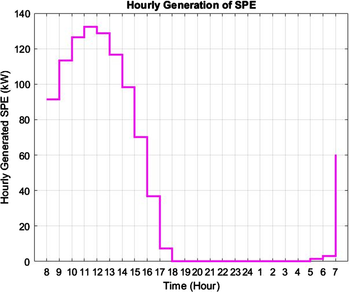
$P_{SPE} = {\begin{matrix} P_{r} (\frac{G_{s}^{2}}{G_{std} * X_{c}}), for 0 < G_{s} > X_{c} \\ P_{r} (\frac{G_{s}}{G_{std}}), for X_{c} < G_{s} > G_{std} \\ P_{r}, for G_{s} > G_{std} \end{matrix}$ (17)

Here, G_s and G_std is the solar irradiance and standard solar irradiance in W/m². X_c is the certain solar irradiance point at considered location. In this article, to show the effect on cost of energy reduction the two different solar profile has been considered. Depending on the solar irradiance data taken from PVGIS, the hourly solar generated power has been evaluated by Equation (17) for SPE-cloudy day and SPE-sunny day. The hourly generated SPE is given in Figs. 1 and 2.

Fig. 1

Hourly generated SPE on SPE-cloudy day.

Fig. 2

Hourly generated SPE on SPE-sunny day.

Here, a 300-kW solar photovoltaic panel has been considered with the assumption of generating 60 percent of its rated power. The hourly SPE generation has been evaluated from Equation (17) by considering the solar irradiance data on earth surface by PVGIS.

The appliance scheduling of different areas is being performed utilizing the flowchart given in Fig. 3. The devices of residential, commercial, and industrial areas use the same flowchart steps to schedule the respective devices. First, the parameters of ACO are initialized and the parameters of ACO are listed in Table 2. After ACO parameters initialization, ants are created that is rand ON/OFF schedule of all available devices are generated with consideration of various constraints. After the creation of ants, the power consumption of each type of device is estimated in different hours of the day. Now, algorithm checks the availability of SPE in each hour and forecasted load is evaluated over the given time span. Now, fitness of all generated schedule is evaluated by using Equation (12). Fitness values corresponds to peak load in each time slot and pheromone matrix is constructed using Equation (13). Evaporation of pheromone is 10 % and Equation (15) is used to evaluate updated pheromone matrix. The algorithm determines the fitness function minimization while updating pheromone matrix. After checking the iteration count algorithm repeats until maximum iteration is reached. Final scheduling of appliances is displayed after completion of all the iterations.

Fig. 3

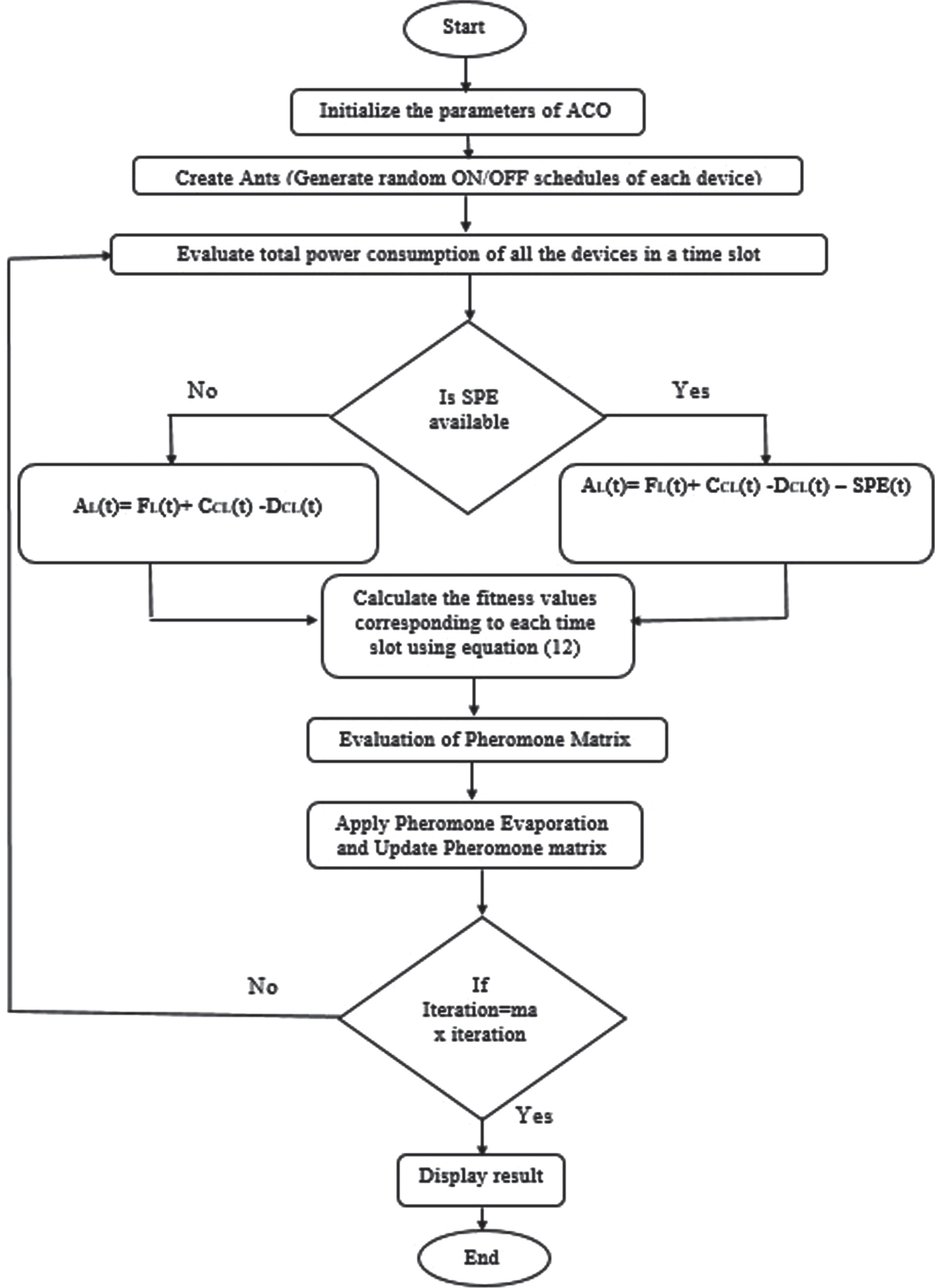
ACO flowchart for Appliance Scheduling.

Table 2

Utility Peak Load (UPL) before and after DSM

Type of loads	UPL before	EA [27]	MFO [28]	BFOA [26]	UPL After DSM with proposed ACO
	DSM				Without SPE	SPE-Cloudy	SPE-Sunny
Residential	1363.6	1114.4	1067.15	1106.3	1042.5	1045.2	1041.5
Commercial	1818.2	1485.2	1459.09	1462.5	1440.7	1425.1	1434.2
Industrial	2727.3	2343.6	2372.75	2338.6	2301.6	2230	2252.8

Here, one point must be noted that the calculation of probability is not required as beta has been assumed to be zero and probability matrix is same as pheromone matrix. So, Equation (18) is used to calculate the probability matrix when beta is non-zero. The number of populations, initial pheromone exponential weight, heuristic exponential weight, and Evaporation Rate are 30, 0.1, 0.02, 0.1 respectively considered in simulation.

5 Result analysis

5.1 Case-1 residential consumers

The non-critical devices in the residential area were sourced from [3]. There are a total of 14 different types of devices, amounting to 2604 devices available for scheduling. For the ACO algorithm used in residential appliance scheduling, the initial population size is set to 30, and the maximum number of iterations is set to 300. The scheduling of residential devices was conducted both with and without the integration of SPE in SG. The forecasted load data in kilowatts (kW) was estimated based on the initial operating time of manageable devices and the base load of the residential area. The ACO algorithm generates random ON and OFF schedules of non-critical devices for their shifting to new operating time slot and evaluates the UPL in the end of each iteration. After comparing this UPL data with desired condition it proceeds for next iteration. To demonstrate the importance and saving in CCE with SPE integrated smart grid, two different solar photovoltaic energy profiles were considered as SPE-cloudy and SPE-cloudy day.

The DSM results for the residential area with SPE- cloudy and SPE-sunny day are shown in Figs. 4 and 5 respectively. The load curves can be clearly seen to follow the desired load curves closely which depicts the effectiveness of proposed ACO algorithm for DSM. Table 2 shows the UPL prior to DSM implementation was 1363.6 kW and reduces to 1042.5, 1045.2 kW and 1041.5 without SPE, with SPE-cloudy day and with SPE-sunny day respectively.

Fig. 4

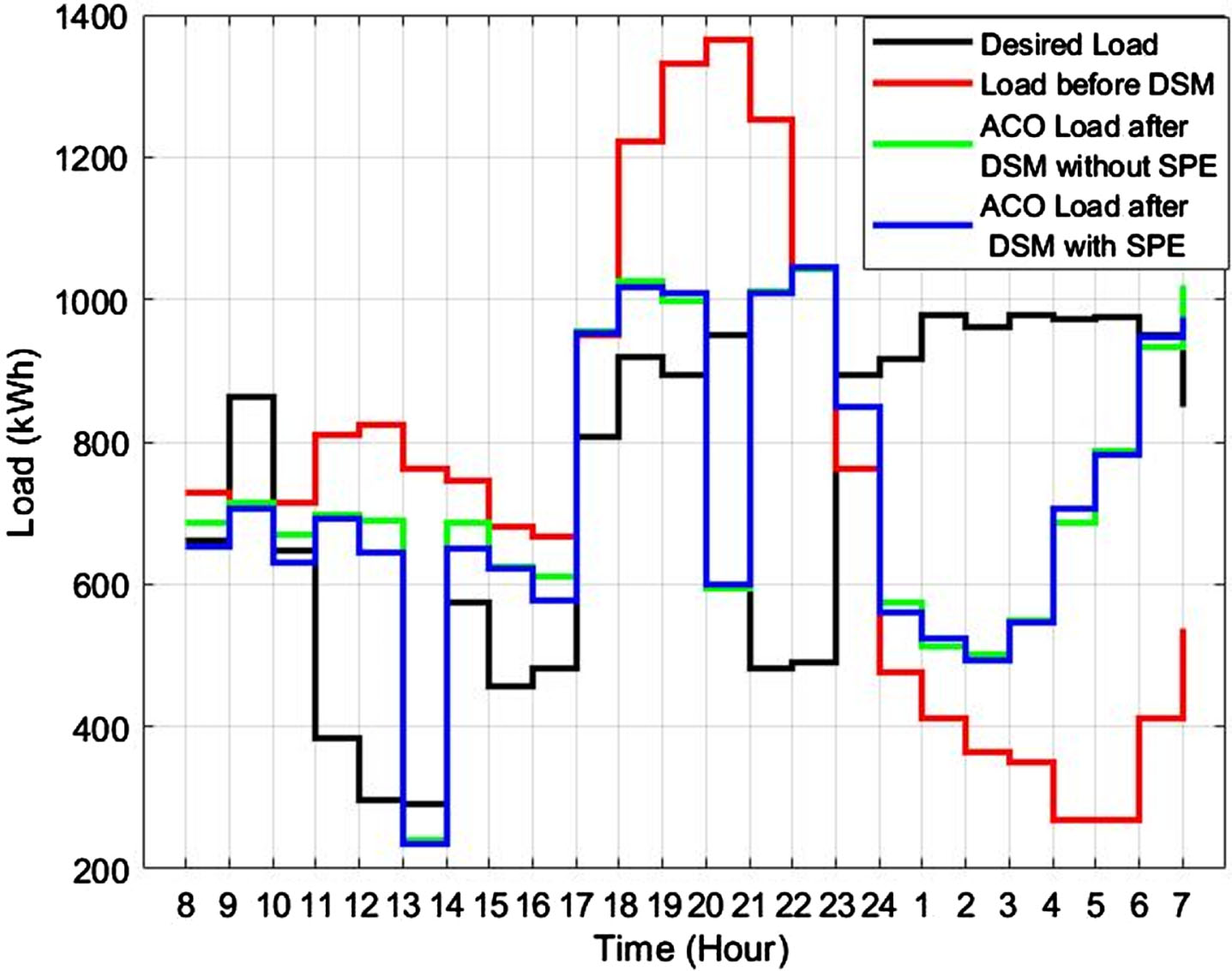
Load curves after DSM in residential area on SPE-cloudy day.

Fig. 5

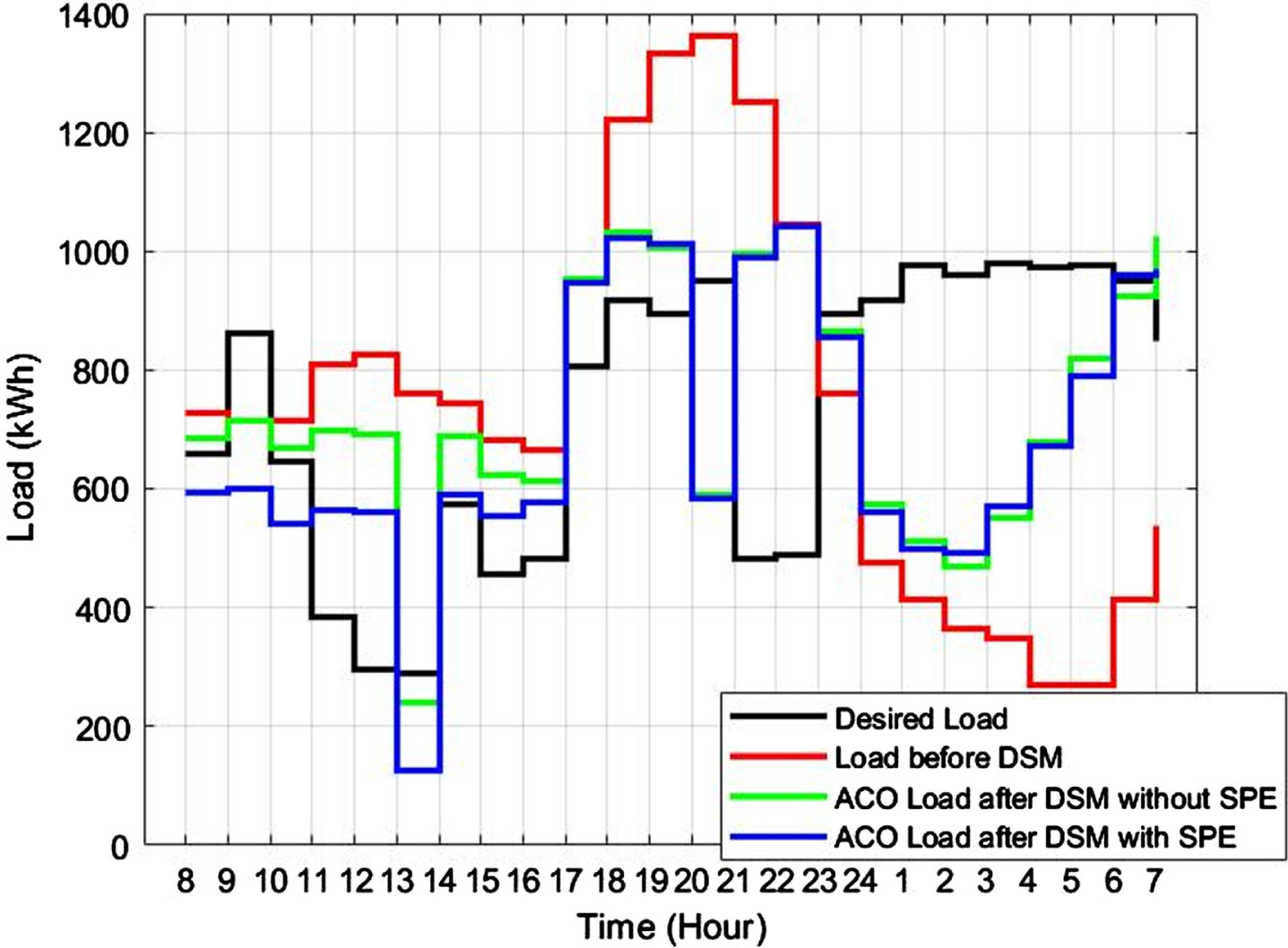
Load curves after DSM in residential area on SPE-sunny day.

The corresponding UPL percentage reductions in the above cases are 23.6%, 23.35%, and 23.6% respectively as shown in Fig. 6. Here, it is also clear that the proposed ACO algorithm gives better results than previously published optimization methods named as EA [27], MFO [28], BFO [26], as shown in Fig. 6. Here, the reduction in peak load is almost the same in without SPE, SPE-cloudy and SPE-sunny cases as the peak occurs in between 22 Hrs-23 Hrs. in which SPE is not available. A greater reduction in UPL is expected to be achieved if SPE availability is there.

Fig. 6

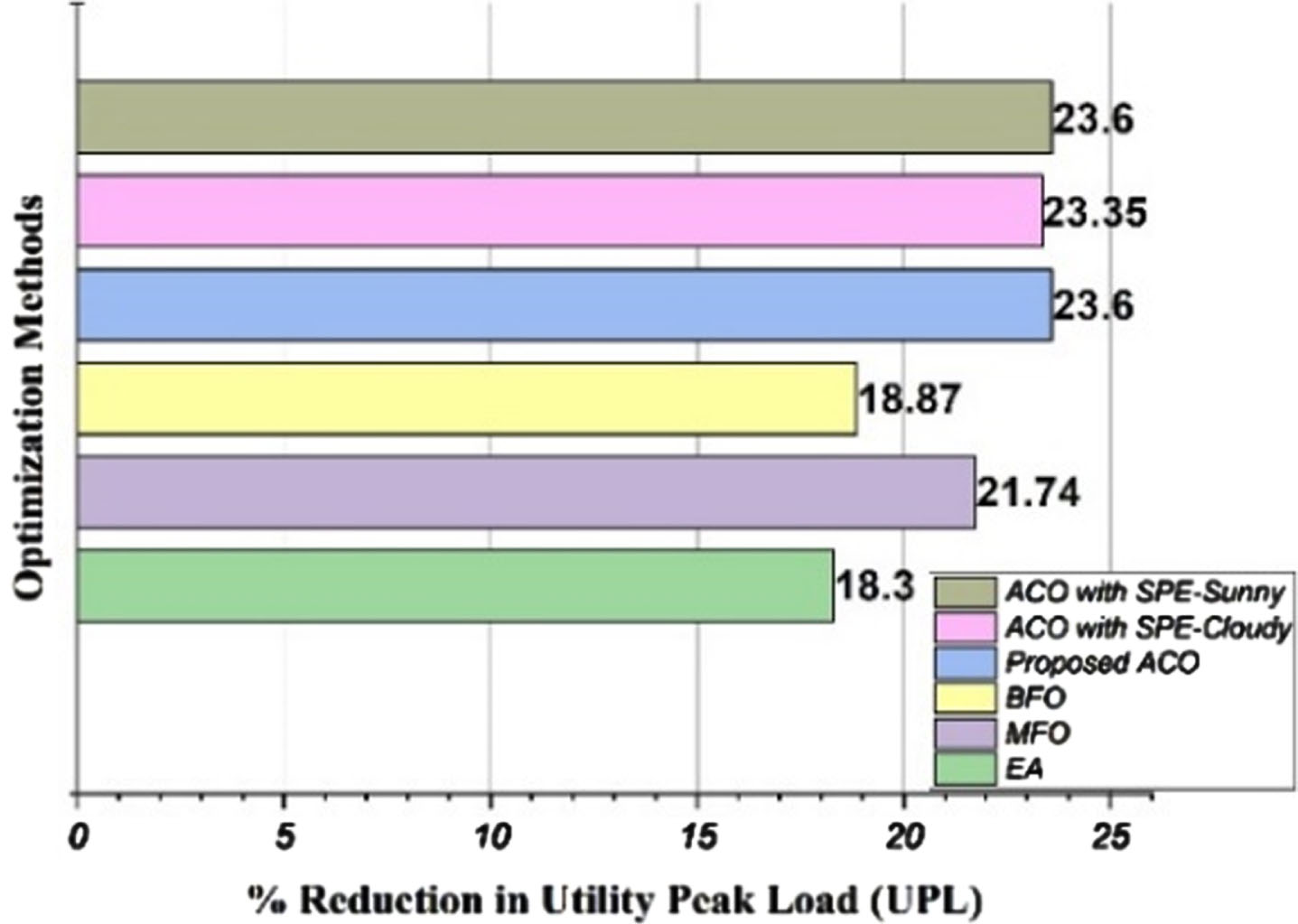
Residential area percentage reduction in UPL.

Similarly, the DSM results shown in Table 3 demonstrate that CCE prior to DSM in residential area was 2302.9 $ and reduces to 2113.8$, 2091.6$ and 1959.3$ in DSM without SPE, with SPE-Cloudy and SPE-sunny respectively. The percentage reductions in CCE are 8.21%, 9.17% and 14.92% respectively as shown in Fig. 7. The 8.21% reduction in CCE thus achieved is better than already published research utilizing EA [27], MFO [28] and BFO [26] optimization methods as clearly seen in Fig. 7. A greater reduction in CCE with SPE-cloudy and SPE-sunny demonstrates that this saving will increase with improvement in SPE profile.

Fig. 7

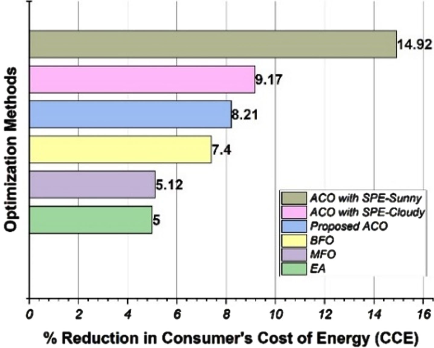
Residential area percentage reduction in CCE.

Table 3

Consumer’s Cost of Energy (CCE) before and after DSM

Type of Loads	CCE Before	EA [27]	MFO [28]	BFOA [26]	CCE After DSM with Proposed ACO
	DSM				Without SPE	SPE-Cloudy	SPE-Sunny
Residential	2302.9	2188.3	2185	2132.5	2113.8	2091.6	1959.3
Commercial	3636	3424.3	3470	3366.9	3289.5	3256.7	3061.5
Industrial	5712	5141.6	5414.98	5135	4599.2	4587.9	4430.6

In this context, it is important to note that the fitness function used in the algorithm is inversely proportional to the objective function described in this article. Therefore, as the number of iterations increases, the fitness function tends towards a maximum value, leading to minimized objective function values. The convergence characteristics of residential area is shown in Figs. 8 and 9 shows that the algorithm converges to its final fitness value in almost 20 iterations.

Fig. 8

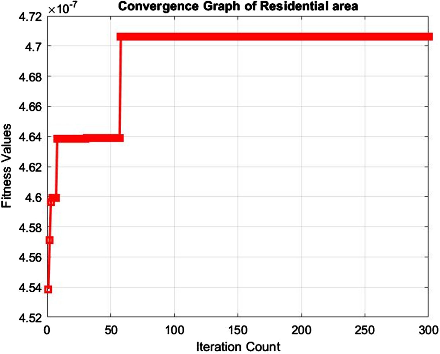
Convergence Curve of residential area with SPE-cloudy day.

Fig. 9

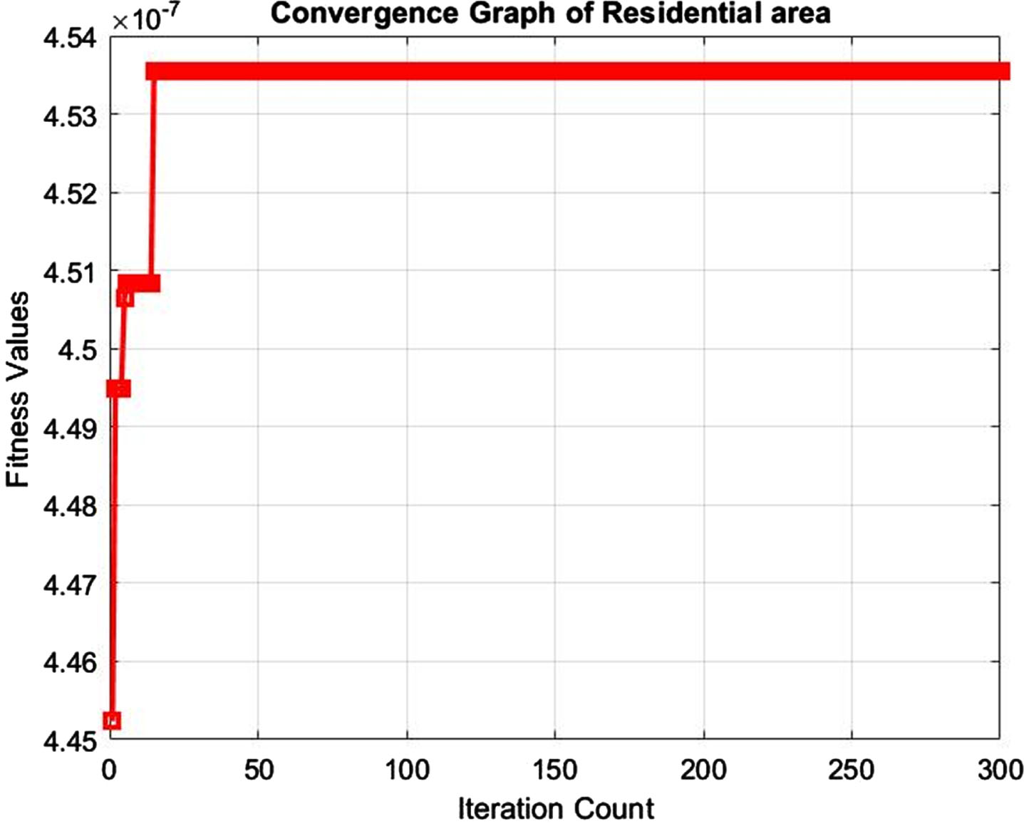
Convergence Curve of residential area with SPE-sunny day.

5.2 Case-2 commercial consumers

The non-critical appliances in the commercial area consist of 808 appliances of 8 different types, with variable operation times and power consumption, as obtained from [3]. The DSM results for the commercial area on both a SPE-cloudy day and a SPE-sunny day are illustrated in Figs. 10 and 11, respectively. The results clearly demonstrate significant reductions in UPL achieved through DSM implementation. The forecasted load curve represents the UPL attributed to the commercial area before the implementation of DSM.

Fig. 10

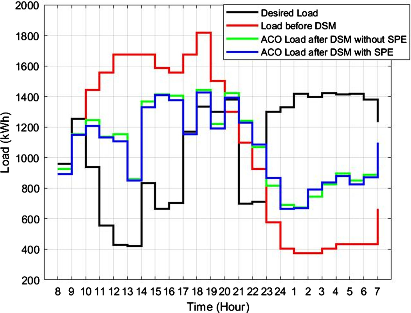
Load curves after DSM in commercial area on SPE-cloudy day.

Fig. 11

Load curves after DSM in Commercial area on SPE-sunny day.

Table 2 presents the DSM results that the UPL was initially 1818.2 kW and reduces to 1440.7 kW without SPE and 1425.1 kW with SPE-cloudy day. On a SPE-sunny day, the UPL decreases to 1434.7 kW from 1440.7 kW.

Figure 12 further highlights a significant reduction of 21.64% without SPE and 21.62% with SPE-cloudy day in UPL, and a reduction of 21.09% with SPE-sunny day. Also, these improvements in UPL is more than the results obtained by other already published optimization methods EA [27], MFO [28], and BFO [26]. The peak occurs in between 18 Hrs.-19 Hrs. in SPE-cloudy and SPE-sunny both the cases. Here it is required to mention that a small amount of SPE is available in SPE-cloudy, but SPE is zero in SPE-sunny, which is clearly mentioned in Figs. 2 and 3.

Fig. 12

Commercial area percentage reduction in UPL.

Moreover, the CCE decreases by 9.81% without SPE and 10.43% with SPE-cloudy day, while the CCE reduces by 15.8% with SPE-sunny day as shown in Fig. 13. Comparing with [26 –28], ACO algorithm gives highest reduction in CCE. The CCE before and after DSM is given in US$ in Table 3. It is evident that the ACO algorithm achieves the highest reduction in both UPL and CCE. The population size and number of iterations used in this study are set at 30 and 300, respectively. The convergence curves are shown in Figs. 14 and 15 reveals that algorithm achieves final fitness in almost 50 and 20 iterations in SPE-cloudy and SPE-sunny respectively.

Fig. 13

Commercial area percentage reduction in CCE.

Fig. 14

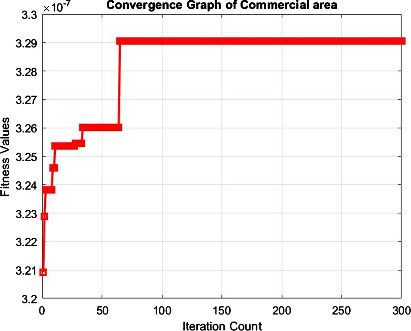
Convergence Curve of commercial area with SPE-cloudy day.

Fig. 15

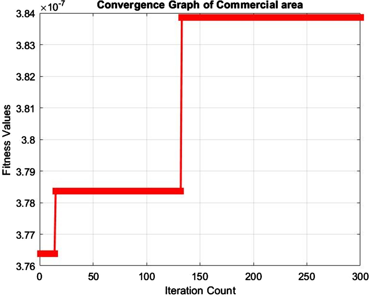
Convergence Curve of commercial area with SPE-sunny day.

5.3 Case-3 industrial consumers

The non-critical appliances of industrial area with different power consumption and different operation time have been considered from [3]. Although these shiftable appliances are the smallest in number as compared with other areas but having large power consumption. The load curves before and after DSM in industrial areas on SPE- cloudy day and SPE-sunny day are shown in Figs. 16 and 17 respectively. Industrial devices’ operation time very high as compared to residential or commercial loads. Figure 16 provides a clear visualization of the reduction in UPL with SPE-cloudy day, while Fig. 17 illustrates the UPL reduction with SPE-sunny day when compared to the load before DSM. The significant decrease in UPL on both days is evident in these figures, particularly when considering the availability of SPE.

Fig. 16

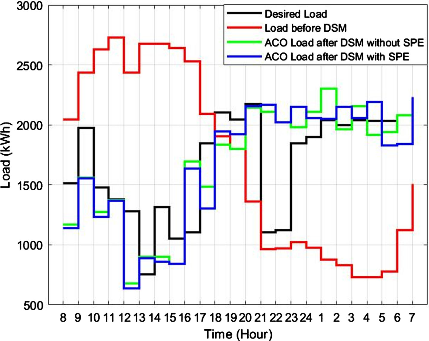
Load curves after DSM in Industrial area on SPE-cloudy day.

Fig. 17

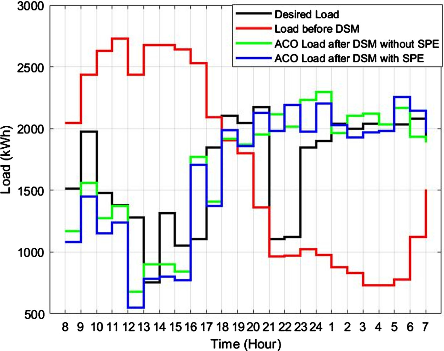
Load curves after DSM in Industrial area on SPE-sunny day.

Table 2 presents the reduction in UPL without SPE and with SPE on the two considered days, along with the corresponding UPL reductions for each case. Prior to DSM implementation, the UPL was recorded as 2727.3 kW. On a cloudy day, it decreases to 2230 kW and on SPE-sunny day UPL is reduced to 2252.8 kW. Notably, Fig. 18 indicates a significant reduction of 15.70% without SPE and 18.23% with SPE-cloudy day, and a reduction of 17.39% with SPE-sunny day. Moreover, the CCE reduction amounts to 19.55% without SPE and 19.67% with SPE-cloudy day, and 22.43% with SPE- sunny day as shown in Fig. 19. The proposed ACO algorithm demonstrates superior performance in terms of achieving maximum reductions in both UPL and CCE, surpassing the results presented in [26 –28]. For the industrial area, the population size in the ACO algorithm is set to 30, with a maximum iteration limit of 300, like the residential and commercial areas. It is worth noting that the industrial area exhibits the highest reduction in CCE when compared to the residential and commercial areas, given its larger power consumption requirements. Also, simulation converges in 150 iterations with SPE-cloudy and in 100 iterations in SPE-sunny day as shown in Figs. 20 and 21 respectively.

Fig. 18

Industrial area percentage reduction in UPL.

Fig. 19

Industrial area percentage reduction in CCE.

Fig. 20

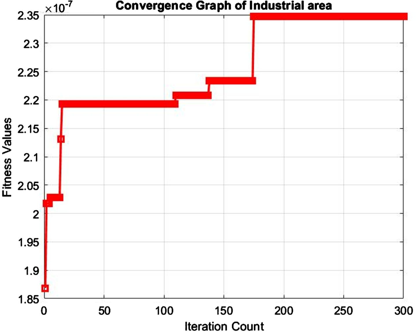
Convergence Curve of Industrial area with SPE-cloudy day.

Fig. 21

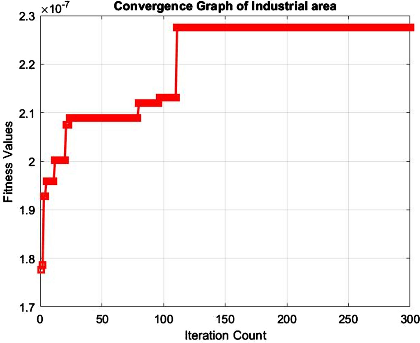
Convergence Curve of Industrial area with SPE-sunny day.

6 Conclusions

The Ant Colony Optimization algorithm has been employed in this study to address the single objective DSM minimization function. Simulations has been carried out in three different areas: residential, commercial, and industrial having appliances of diverse power consumption and operating time. In this study, the reduction in CCE and UPL has been observed in all the areas considered without and with SPE.

After a consolidated analysis of all the considered areas, it has been observed that maximum reduction in UPL occurs in residential areas having maximum number and types of devices. The maximum reduction in CCE was observed in the industrial area with highest kW of total load. This observation shows that higher saving in CCE and more reduction in UPL can be achieved when this algorithm is used for the area having large number of devices of various types with higher kW of total load.

The use of multi-objective approach considering UPL and CCE as minimization function with latest optimization techniques may result more reduction in UPL and CCE. The utilization of different renewable energy sources, such as Solar Photovoltaic Energy (SPE), presents a promising avenue for future integration among residential, commercial, and industrial stakeholders. Notably, even without the integration of SPE, the DSM results demonstrate a reduction in Utility Peak Load (UPL) and a decrease in Consumer’s Cost of Energy (CCE). By implementing this DSM framework for grouped loads, the need for load shedding can be minimized, thereby improving the overall power supply reliability. The reduction in CCE has been observed across all areas, with greater reductions achieved as the penetration of renewable energy increases. To fully capitalize on the cost savings potential, implementing this approach on a large-scale network within a smart grid environment would yield manifold benefits.

References

Vashishtha

and Ramachandran

, Multicriteria evaluation of demand side management (DSM) implementation strategies in the Indian power sector, Energy 31(12) (2006), 2210–2225. doi: 10.1016/j.energy.2005.10.005.

Yadav

R.K.

, Bhadoria

V.S.

, Hrisheekesha

P.N.

Technical and Financial Assessment of a Grid Connected SolarPVNet Metering System for Residential Community, in 2019 2nd International Conference on Power Energy Environment and Intelligent Control, PEEIC 2019, 2019. doi: 10.1109/PEEIC47157.2019.8976657.

Yadav

R.K.

, Hrisheekesha

P.N.

and Bhadoria

V.S.

, Grey Wolf Optimization Based Demand Side Management in Solar PV Integrated Smart Grid Environment, IEEE Access 11 (2023), 11827–11839. doi: 10.1109/ACCESS.2023.3241856.

Ramesh

, Saini

R.P.

DemandSide Management based techno-economic performance analysis for a stand-alone hybrid renewable energy system of India, Energy Sources, Part A: Recovery, Utilization and Environmental Effects, 2020, doi:10.1080/15567036.2020.1851820.

Zehir

M.A.

, Bagriyanik

Demand Side Management by controlling refrigerators and its effects on consumers, in Energy Conversion and Management (2012), 238–244. doi: 10.1016/j.enconman.2012.05.012.

Niharika and Mukherjee

, Day-ahead demand side management using symbiotic organisms search algorithm, IET Generation, Transmission and Distribution 12(14) (2018), 3487–3494. doi: 10.1049/iet-gtd.2018.0106.

Rahman

, Rinaldy , An efficient load model for analyzing demand side management impacts, in IEEE Transactions on Power Systems, 8(3) (1993), 1219–1226. doi: 10.1109/59.260874.

Kirschen

D.S.

, Demand-side view of electricity markets, IEEE Transactions on Power Systems 18(2) (2003), 520–527. doi: 10.1109/TPWRS.2003.810692.

K.-H.

and Sheble

G.B.

, Direct load control-A profit-based load management using linear programming, in IEEE Transactions on Power Systems 13(2) (1998), 688–694. doi: 10.1109/59.667401.

10.

Deh-Chang Wei , Nanming Chen , Air conditioner direct load control by multi-pass dynamic programming, in IEEE Transactions on Power Systems 10(1) (1995), 307–313. doi: 10.1109/59.373916.

11.

Cohen

A.I.

and Wang

C.C.

, An optimization method for load management scheduling Power Systems, IEEE Transactions on 3(2) (1988), 612–618.

12.

Yao

, Chang

W.C.

and Yen

R.L.

, An iterative deepening genetic algorithm for scheduling of direct load control, IEEE Transactions on Power Systems 20(3) (2005), 1414–1421. doi: 10.1109/TPWRS.2005.852151.

13.

Faranda

, Pievatolo

and Tironi

, Load shedding: A new proposal, IEEE Transactions on Power Systems 22(4) (2007), 2086–2093. doi: 10.1109/TPWRS.2007.907390.

14.

Yadav

R.K.

, Hrishikesha

P.N.

and Bhadoria

V.S.

, Lowest Tariff Load Shifting Demand Side Management Technique in Smart Grid Environment, International Journal of Social Ecology and Sustainable Development 13(2) (2022). doi: 10.4018/IJSESD.302468.

15.

Yadav

R.K.

, Hrishikesha

P.N.

, Bhadoria

V.S.

A nature inspired strategy for demand side management in residential sector with smart grid environment, in Proceedings of the 2020 9th International Conference on System Modeling and Advancement in Research Trends, SMART 2020, Institute of Electrical and Electronics Engineers Inc. (2020), 235–239. doi: 10.1109/SMART50582.2020.9337101

16.

Tsagarakis

, Camilla Thomson

, Collin

A.J.

, Harrison

G.P.

, Kiprakis

A.E.

and McLaughlin

, Assessment of the Cost and Environmental Impact of Residential Demand-Side Management, IEEE Trans Ind Appl 52(3) (2016), 2486–2495. doi: 10.1109/TIA.2016.2516478.

17.

Althaher

, Mancarella

and Mutale

, Automated Demand Response from Home Energy Management System Under Dynamic Pricing and Power and Comfort Constraints, IEEE Trans Smart Grid 6(4) (2015), 1874–1883. doi: 10.1109/TSG.2014.2388357.

18.

Conejo

A.J.

, Morales

J.M.

and Baringo

, Real-time demand response model, IEEE Trans Smart Grid 1(3) (2010), 236–242. doi: 10.1109/TSG.2010.2078843.

19.

Zhao

, Lee

W.C.

, Shin

and Bin Song

, An optimal power scheduling method for demand response in home energy management system, IEEE Trans Smart Grid 4(3) (2013), 1391–1400. doi: 10.1109/TSG.2013.2251018.

20.

IEEE, 2012 IEEE PES Innovative Smart Grid Technologies. DOI: 10.1109/ISGT19241.2012.

21.

IEEE Robotics and Automation Society, Annual IEEEComputer Conference, C. Annual IEEE International Conference on CYBER Technology in Automation, IEEE-CYBER 5 2015.06.08-12 Shenyang, and IEEE CYBER 5 2015.06.08-12 Shenyang, 2015 IEEE International Conference on CYBER Technology in Automation, Control, and Intelligent Systems (CYBER) 8-12 June 2015, Shenyang, China.

22.

Setlhaolo

, Xia

and Zhang

, Optimal scheduling of household appliances for demand response, Electric Power Systems Research 116 (2014), 24–28. doi: 10.1016/j.epsr.2014.04.012.

23.

Remani

, Jasmin

E.A.

, Ahamed

T.P.I.

Residential load scheduling considering maximum demand using binary particle swarm optimization, International Journal of Advanced Intelligent Paradigms 17, pp 29–43, DOI: 10.1504/IJAIP.2020.10028510.

24.

Rahim

et al. Exploiting heuristic algorithms to efficiently utilize energy management controllers with renewable energy sources, Energy Build 129 (2016), 452–470. doi: 10.1016/j.enbuild.2016.08.008.

25.

Javaid

et al. An Intelligent Load Management System with Renewable Energy Integration for Smart Homes, IEEE Access 5 (2017), 13587–13600. doi: 10.1109/ACCESS.2017.2715225.

26.

Priya Esther

, Shivarama Krishna

, Sathish Kumar

, Ravi

Demand side management using bacterial foraging optimization algorithm, in Advances in Intelligent Systems and Computing, Springer Verlag (2016), 657–666. doi: 10.1007/978-81-322-2755-7_68.

27.

Logenthiran

, Srinivasan

and Shun

T.Z.

, Demand side management in smart grid using heuristic optimization, IEEE Trans Smart Grid 3(3) (2012), 1244–1252. doi: 10.1109/TSG.2012.2195686.

28.

Zeeshan

and Jamil

, Adaptive Moth Flame Optimization based Load Shifting Technique for Demand Side Management in Smart Grid, IETE J Res 68(1) (2022), 778–789. doi: 10.1080/03772063.2021.1886607.

29.

, Tazvinga

and Xia

, Demand side management of photovoltaic-battery hybrid system, Appl Energy 148 (2015), 294–304. doi: 10.1016/j.apenergy.2015.03.109.

30.

Chiu

T.C.

, Shih

Y.Y.

, Pang

A.C.

and Pai

C.W.

, Optimized Day-Ahead Pricing with Renewable Energy Demand-Side Management for Smart Grids, IEEE Internet Things J 4(2) (2017), 374–383. doi: 10.1109/JIOT.2016.2556006.

31.

Remani

, Jasmin

E.A.

and Ahamed

T.P.I.

, Residential Load Scheduling with Renewable Generation in the Smart Grid: A Reinforcement Learning Approach, IEEE Syst J 13(3) (2019), 3283–3294. doi: 10.1109/JSYST.2018.2855689.

32.

Puttamadappa

, Parameshachari

B.D.

Demand side management of small-scale loads in a smart grid using glowworm swarm optimization technique, Microprocessors and Microsystems,Volume 71, 2019, 102886, ISSN 0141-9331, ttps://doi.org/10.1016/j.micpro.2019.102886.

33.

Arumugham

et al. An Artificial-Intelligence-Based Renewable Energy Prediction Program for Demand-Side Management in Smart Grids, Sustainability (Switzerland) 15(6) (2023). doi: 10.3390/su15065453.

34.

M. IEEE Systems and Institute of Electrical and Electronics Engineers, Intelligent Systems Design and Applications (ISDA), 2014 14th International Conference on: date, 28-30 Nov. 2014.

35.

Merkle

, Middendorf

and Schmeck

, Ant colony optimization for resource-constrained project scheduling, IEEE Transactions on Evolutionary Computation 6(4) (2002), 333–346. doi: 10.1109/TEVC.2002.802450.

36.

Preisler

, Renz

, Dethlefs

Ant-Colony based Self-Optimization for Demand-Side-Management Ant-Colony based Self-Optimization for Demand-Side-Management. [Online]. Available: https://www.researchgate.net/publication/272173725.

37.

Abualigah

, Yousri

, Abd Elaziz

, Ewees

A.A.

, Al-qaness

M.A.A.

and Gandomi

A.H.

, Aquila Optimizer: A novel meta-heuristic optimization algorithm, Comput Ind Eng 157, Jul. 2021. doi: 10.1016/j.cie.2021.107250.

38.

Abualigah

, Diabat

, Mirjalili

, Abd Elaziz

and Gandomi

A.H..

, The Arithmetic Optimization Algorithm, Comput Methods Appl Mech Eng 376 (2021). doi: 10.1016/j.cma.2020.113609.

39.

Dorigo

, Birattari

and Stutzle

, Ant colony optimization, in IEEE Computational Intelligence Magazine, 1(4) (2006), 28–39. doi: 10.1109/MCI.2006.329691.

40.

Maniezzo

, Carbonaro

Ant Colony Optimization: An Overview. In: Essays and Surveys in Metaheuristics. Operations Research/Computer Science Interfaces Series, vol 15. Springer, Boston, MA. (2002) https://doi.org/10.1007/978-1-4615-1507-4_21.

41.

Rahim

et al. Ant colony optimization-based energy management controller for smart grid, in Proceedings - International Conference on Advanced Information Networking and Applications, AINA, Institute of Electrical and Electronics Engineers Inc. (2016), 1154–1159. doi: 10.1109/AINA.2016.163.

42.

Blum

, Ant colony optimization: Introduction and recent trends, (4), Physics of Life Reviews 2 (2005), 353–373. doi: 10.1016/j.plrev.2005.10.001.

43.

Laitsos

V.M.

, Bargiotas

, Daskalopulu

, Arvanitidis

A.I.

and Tsoukalas

L.H.

, An incentive-based implementation of demand side management in power systems, Energies (Basel) 14(23) (2021). doi: 10.3390/en14237994.

44.

Oda

E.S.

, El Hamed

A.M.A.

, Ali

, Elbaset

A.A.

, El Sattar

M.A.

and Ebeed

, Stochastic optimal planning of distribution system considering integrated photovoltaic-based dg and dstatcom under uncertainties of loads and solar irradiance, IEEE Access 9 (2021), 26541–26555. doi: 10.1109/ACCESS.2021.3058589.

Parameter	Parameter
Name	Description
D_L(t)	Desired load at time t
F_L(t)	Forecasted load at time t
A_L (t)	Actual load at time t
O_FN(t)	Objective function
L_BDSM(t)	Load before DSM at time t
L_ADSM(t)	Load after DSM at time t
B_L (t)	Base Load
C_CL (t)	Load connected at time t
D_CL (t)	Load Disconnected at time t
TOUP	Time of Use Pricing
CCE	Consumer’s Cost of Energy
UPL	Utility Peak Load
PAR	Peak to Average Ratio
$δ T_{a, b}^{c}$	Amount of Pheromone deposited on path a,b by cth ant
P_a,b	Probability of path a, b
$T_{a, b}^{c}$	level of pheromone on a path
φ _a,b	Represents the heuristic information
G_S	solar irradiance
G_STD	standard solar irradiance in W/m²
P_R	SPE availability profile
X_C	certain solar irradiance points at considered location