
Abstract
In order to solve the problem of discrete manufacturing customization and personalized production scheduling, considering the influence of manual labor on processing time, we propose a multi-objective Hybrid Job-shop Scheduling with Multiprocessor Task(HJSMT) problem with cooperative effect model. Based on the actual production, two optimization objectives are set, i. e. minimizing the maximum completion time and the total tardiness. Firstly, considering the situation where workers’ cooperation reduces job processing time, the cooperative effect of workers co-processing is considered by referring to the learning effect curve in the model. Subsequently, we develop an Improved Non-dominated Sorting Genetic Algorithm-II (INSGA-II) to solve the multi-objective HJSMT problem by improving Precedence Operation Crossover (POX) and Multiple Mutations (MM) operations. Finally, the scheduling results and the C values are compared with other algorithms to verify the effectiveness of the algorithm. Simultaneously, the multi-objective HJSMT problem with the cooperative effect is solved by the INSGA-II algorithm, and the experimental results also demonstrate the superior performance of the algorithm.
Keywords
Introduction
With all kinds of manufacturing enterprises have been transformed and upgraded to intelligence, informatization and digitalization, this has led to a trend of intelligent scheduling in workshops. Many large, single-piece discrete manufacturing workshops no longer rely on mass production modes and instead produce personalized and customized products. Unlike small batch manufacturing, which cannot use flow line or robot production, discrete enterprise workshops now have features that allow for parallel processing, processing upgrades, multi-processor tasks, etc. In many cases, the job requires at least one (≥1) machine or worker to process simultaneously, making the original single-processor model of workshop scheduling no longer applicable.
The Job-shop Scheduling Problem (JSP) and Flow-shop Scheduling Problem (FSP) are the most common types of shop scheduling problems, which have been extensively researched with respect to machines, time and various objective functions. To better address modern production needs, hybrid scheduling types such as the Flexible Flow-shop Scheduling (FFS), Flexible Job-shop Scheduling (FJS), Flexible Open-shop Scheduling (FOS), Hybrid Flow-shop Scheduling with multiprocessor task (HFSMT) and Hybrid Job-shop Scheduling with Multiprocessor Task (HJSMT) problem have emerged [16]. One of these models, HJSMT problem [22], is a combination of the classical Job Shop Scheduling (JSP) problem and Multiprocessor Task Scheduling (MTS), where several jobs to be processed have several different operations and an operation for a job requires a set of processors instead of a single processor. However, relatively little research has been done on this problem. In their research, Wang et al. addressed the challenge of hybrid scheduling in network parallel computing, where both multi-step and multi-processor tasks are present [21]. To solve this problem, they combined the PSO algorithm with simulated annealing. Similarly, Fan et al. established a hybrid HJSMT problem model and designed a hybrid genetic algorithm for simulation experiments for the workshop production problem in modern steel manufacturing enterprises [17]. Wang et al. proposed and implemented an improved brainstorming algorithm to solve the non-hybrid multi-processor combined production batch scheduling model discussed in the article [23].
In real manufacturing plants, not all operations are done by machines, workers also process or even cooperate in processing. When workers collaborate on a job, the time spent on processing decreases, resulting in a cooperative effect that can reduce workers’ working time, decrease shop floor energy consumption and improve overall efficiency.
Traditional job-shop scheduling problems typically focus on a single optimization objective. However, with increasing market competition, multi-objective optimization studies of job-shop scheduling have become more important over the last decade. Researchers consider objectives such as minimizing maximum completion time, reducing energy consumption, minimizing total tardiness, and managing machine workload. Wang et al. investigated the Flexible Job-shop Scheduling Problem (FJSP) model to reduce energy consumption [19], while Wang et al. considered completion time, total energy consumption, total tardiness, and total machine load as objectives in their FJSP model [23]. Li et al. included machine workload in addition to total work time in the FJSP model [12], and Amiri et al. considered the maximum completion time, number of delayed jobs, and total flow time for the automated flexible job-shop [9]. To address these problems, researchers such as Deb et al. [14], Coello et al. [4], and Zitzler et al. [34] proposed classical solution algorithms like NSGA-II, MOPSO, and SPEA2. Moreover, many scholars have used improved intelligent algorithms to solve the job-shop scheduling problem. For instance, Erfan et al. used a hybrid NSGA-II and local search algorithm to solve the dynamic facility layout and job-shop scheduling problems, simultaneously [8]. Moslehi and Mahnam developed the MOPSO+LS algorithm by adding a local search algorithm to PSO to solve the multi-objective FJSP model [11]. Sun used the grey wolf optimization algorithm along with a non-dominated ranking genetic algorithm to solve a FJSP problem with three objectives [29]. Leo et al. proposed three multi-objective scatter search hybrid algorithms to solve the multi-objective JSP problem [18]. Xu et al. used the flower pollination algorithm to solve a multi-objective model for flexible job-shop scheduling that used triangular fuzzy number representation [27]. Aghajani and Fouladi proposed a bi-objective mathematical model of the FJSP problem and used an improved NSGA-II to find the Pareto optimal solution [3]. Additionally, An et al. designed two modified precedence operation crossover (named MPOX1 and MPOX2) strategies to inherit and maintain more information from the parent to the child in algorithm to deal with integrated optimization of real-time order acceptance and FJSP rescheduling with multi-level imperfect maintenance constraints [30], and designed an enhanced precedence operation crossover (EPOX) to deal with joint optimization of preventive maintenance and FJSP rescheduling with processing speed selection [31].
The current shift and upgrade of production methods in discrete manufacturing companies favor the use of the HJSMT problem model, which is best suited for the new discrete manufacturing shop. The cooperative effect needs to be considered when simulating actual production as it can reduce workers’ working time, decrease job-shop energy consumption, and improve overall efficiency. Additionally, with the increase of the production-to-order model, delivery time requirements are increasing, and companies need to focus on production goals beyond minimizing maximum completion time. This paper innovates on the research problem by considering the influence of worker cooperative effect on scheduling production, taking the HJSMT problem with cooperative effect as the research object, and minimizing both total tardiness and maximum completion time as the scheduling objectives.
The paper is organized as follows. In the next section, the multi-objective HJSMT problem and the cooperative effect are defined, and a mathematical model is constructed. In Section 3, a suitable optimization algorithm based on the original classical algorithm NSGA-II is designed by improving operations such as POX crossover and multi-round variation. In Section 4, simulation experiments compare the proposed algorithm to verify its effectiveness and analyze the impact of the cooperative effect at different levels of cooperation ratio (70%, 80%, and 90%). Finally, conclusions are given in Section 5.
Model construction of multi-objective HJSMT problem with cooperative effect
Multi-objective HJSMT problem description
According to the HJSMT problem characteristics, it’s defined as: processing a set of jobs J ={ J1, J2, …, J n } on m processors with q i operations J i ={ O ij |j = 1, 2, …, q i } for each job that must be processed in a certain sequence and with fixed processing times, and each operation requires processing by multiple (≥1) designated processors simultaneously. This paper aims to develop a suitable scheduling plan that adheres strictly to the process route and processing time of each operation.
The problem has several conditions: Only one operation can be processed at a time on a processor; Each processor is unique and cannot be mixed; No sequential order exists between operations of different jobs; The process cannot be interrupted once it has started; There are no unexpected situations like raw material shortages, orders insertion or machine damage.
This paper sets the objectives of minimizing maximum completion time and minimizing total tardiness. In practical applications, objectives can be tailored to suit the importance of orders, machine loads, delivery requirements, etc.
Cooperative effect
During the actual production process, repeated cooperation among two or more workers can lead to a reduction in actual working time due to improvements in coordination and cooperation proficiency. This phenomenon is defined as the cooperative effect in this paper. In HJSMT problem, each operation of the job is not necessarily processed by one processor; it may be processed by several processors simultaneously. In this case, the processor processing can be considered equivalent to worker processing.
In this scenario, assume that there is an original processing te T. The cooperative effect hypothesis suggests that when the same worker combinations reappear for combined processing, the cooperation proficiency increases, leading to increased processing efficiency and a reduction in actual processing time below T. For example, as shown in Table 1, the worker combinations required in the first step of job J3 are M1 and M3, and the same worker combination appears again in step 2 of job J2. As a result of this repetition, the actual processing time will be smaller than the original processing time.
Examples of cooperative effect in HJSMT problem
Examples of cooperative effect in HJSMT problem
Previous scholars have conducted limited research on the cooperative effect. However, some scholars have studied the learning effect in job-shop scheduling problems, which implies that workers become more familiar with equipment or operations through continuous work, leading to an increase in proficiency and a reduction in processing time [1, 26]. Due to its similarity with the cooperative effect, this paper refers to the position-based learning effect curve [7, 10] and uses it to express the actual processing time while considering the cooperative effect in the Equation (1):
Here, y
k
represents the original processing time of the job processed at the k-th position, while y1 represents the processing time of the job processed at the first position,
In summary, this paper considers the cooperative effect in HJSMT problem processing, resulting ian actual processing time of t q = y q × r α, y q set as the original processing time of operation q; r is the number of repeated combinations of workers. For instance, in Table 1, for step 1 of job J3, the same combination of workers is required as for step 2 of job J2. Therefore, if step 1 of J3 is completed first, when step 2 of J2 is processed again, it becomes the second occurrence of the same worker combination, which leads to a value of r = 2.
Referring to the literature [13], the symbols in the model are defined as shown in Table 2.
Symbol definition
Symbol definition
Based on the previous equation (4), when l takes the values of 90%, 80%, and 70%, the corresponding values α are -0.15, -0.32, and -0.51, respectively. For any task J i ∈ S in the set S consisting of q i operations, there is J i = {O ij |j = 1, 2, …, q i } and J i ∈ I. Moreover, for the start and finish dummy operations, m σ = m μ = ∅ , t σ = t μ = 0, x μ denotes the maximum completion time. Additionally, the notation A = {{a, b} : a, b ∈ J, anda < b, {a, b} ∈ A} means terations a and b belong to the same job and that operation a must be finished before operation b begins. The notation B = {{a, b} : a ∈ J, b ∈ J′withJ, J′ ∈ S, J ≠ J′ and C a ∩ C b ≠ ∅} , {a, b} ∈ B signies that operations a and b belong to different jobs but require at least one common processor for processing.
The mathematical model that addresses the multi-objective HJSMT problem is defined below.
Objective function:
Constraints:
In Equation (5), the function f1 represents the objective ominimizing the maximum completion time, while f2 represents the objective of minimizing the total tardiness. Equation (6) represents the operation sequence constraint; Equation (7) corresponds to the processor resource constraint; and Equation (8) denotes the “start and finish dummy operation” constraint.
Based on the characteristics of multi-objective job-shop scheduling problem, scholars have proposed many classical algorithms to solve it, among which the fast non-dominated sorting genetic algorithm NSGA-II [14] is widely used. However, this algorithm cannot be directly applied to the HJSMT problem in this paper, and has defects such as easily falling into local optimality. Therefore, this paper improved the NSGA-II algorithm to retain its original advantages and achieve better performance in solving the problem at hand.
Code mechanism
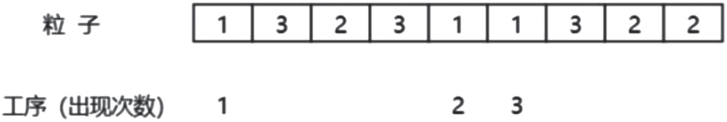
Coding is the key to the success of particle swarm algorithm optimization. This paper utilizes a commonly used operation-based coding method for particle swarm algorithm optimization. The encoded particle represents a scheduling, where the number of operations for job i is denoted by |J
i
|. The particle is a vector of length equal to the total number of operations, that is
Example of encode and decode.
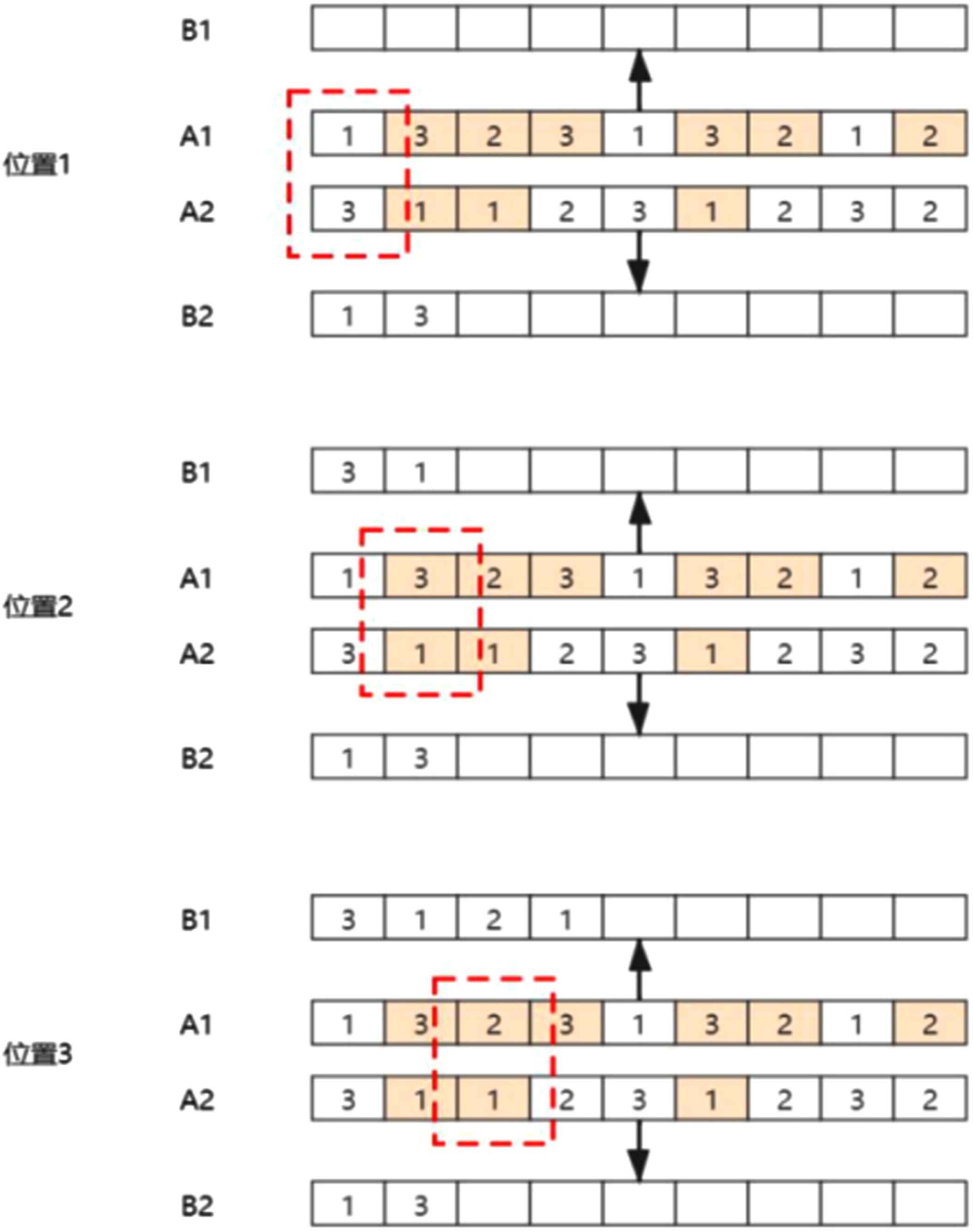
This paper uses the Improved Priority Operation Crossover (IPOX) algorithm [5] depicted in Figs. 2 and 3. A1 and A2 represent the two particles tbe crossed, while B1 and B2 represent the resulting new particles. The algorithm proceeds as follows and runs as Algorithm 2:
Example of IPOX.

Example of IPOX.
Step 1: Randomly divide the task set S ={ J i |i = 1, 2, …, n } into two subsets, S1 and S2.
Step 2: Place the elements belonging to S1 in A1 and the elements belonging to S2 in A2 into B1 without changing their positions.
Step 3: Place the element belonging to S2 in A1 and the element belonging to S1 in A2 into B2 without changing their positions.
Step 4: Calculate the adaptation values for B1 and B2 and select the Pareto dominant particles. If they are not dominated by each other, randomly select one of them.
This paper implements a swap operation for particle variation, where two random integers within the range of the particle length are generated and the numbers at those positions are exchanged. For instance, if particle p is (2, 1, 3, 1, 3, 1, 1, 2, 3, 2) and the particle length is 9, two random integers in the range [1, 9] are generated. Assuming the random numbers are 2 and 5, the numbers at position 2 are swapped with those asition 5 to generate the new particle (2, 3, 3, 1, 1, 1, 1, 2, 3, 2).
In this paper’s particle update process, particles are not ted according to the mutation probability b instead replaced by mutation 20 times using Multiple Mutations (MM), as shown in Algorithm 3 the initial particle dominates the particle after each mutation, it is not replaced.f the new particle Pareto dominates, it replaces the old one. When they do not dominate eother, one is randomly chosen.
Fast non-dominated sorting
The Pareto finding step of NSGA-II, designed by Deb [14], uses the fast non-dominated sort algorithm. Given a population P and individuals p in the population, the algorithm computes the number of individuals n p in the population that are dominated by individuals p and the set S p of individuals in the population dominated by individuals p. The main steps of the algorithm are as follows [6] and are implemented according to Algorithm 4:
Step 1: Save all individuals n p = 0 in the population in the set F i ;
Step 2: For each individual i in F1, let s i be the set of individuals dominated by i, iterate through the individuals l in n l = n l - 1, and store the individuals l of n l = 0 in the set N;
Step 3: Record the stratum of individuals in F1 as the first non-dominated stratum, set N as the current set, and repeat the above steps until the population completes the hierarchy.
Congestion distance and elite retention strategy
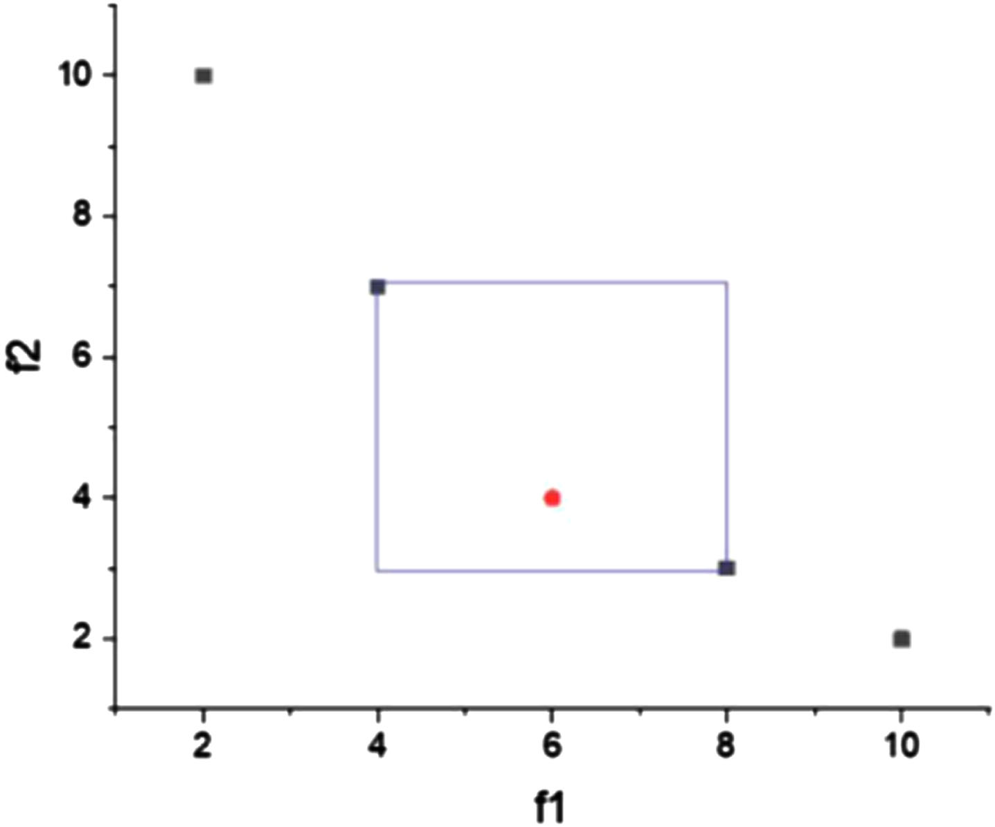
In the case of two objective functions, the crowding dtance can be calculated as the perimeter of the rectangle formed by the adjacent solutions on both sides, with these two solutions as vertices of the diagonal. Figure 4 illustrates tconcept with five points representing t solutions at the same level, where the cwding distance of the third solution iequal to the perimeter of the rectangle with the second and fourth points as diagonals. A larger crowding distance indicates a more dispersed current solution and greater differences between it and surrounding solutions.
Crowding-distance icon.
Conversely, a smaller crowding distance represents a denser current solution and higher similarity to surrounding solutions. The crowding distance of boundary particles in the same layer is recorded as infinity, and every other particle receives a crowding distance by running Algorithm 5. Following the elite retention strategy, particles with smaller layers are preferred for the next generation. When solutions are in the same layer, those with larger crowding distances should be selected first for better diversity of solutions
The improved multi-objective genetic algorithm can be summarized into the following steps:
Step 1: Set the parameters, including population size (popsize), maximum number of iterations (N), and crossover probability (Pm).
Step 2: Initialize the population using process-based encoding. Generate particles twice the size of the population and select popsize particles as the initial particles to enter the iterative process.
Step 3: Select parent particles. Generate two random positive integers, rand1 and rand2, select particles A and B from these positions, and choose the particle with superior Pareto dominance in A and B to put into the parent particle set. If they are not dominated by each other, choose the particle with a greater crowding distance. If A and B are not dominated by each other and have the same crowding distance, choose one of them randomly to put into the parent particle set.
Step 4: Perform crossover operation on the parent particles. Take out two parent particles at a time and perform the Improved Priority Operation Crossover (IPOX) operation to generate two new particles. Calculate their fitness values and add them to the child particle set.
Step 5: Apply a modified Multiple Mutations (MM) operation to the particles in the child particle set to generate new particles.
Step 6: Merge the parent and child generations and optimize the particle set. Sort the particles using fast non-dominated sorting and select popsize particles for the next iteration using a combination of the crowding distance and the elite retention strategy.
Step 7: Check if the termination condition is met. If it is, output the final selection of Pareto non-dominated solutions. Otherwise, go back to step 3.
Experimental simulation and result analysis
Experimental simulation of INSGA-II algorithm
In this paper, the delivery time is determined based on the standard problem of job-shop scheduling proposed by scholars [20, 32]. For a problem with 10 jobs, the processing times of the 2nd and 3rd jobs are added together,nd their sum is multiplied by 1.5 to set their delivery times. The delivery time for the 10th job is set as the sum of its processing time, while t delivery time for the remaining jobs is set aice the sum of their corresponding processing time. For a problem with 5 jobs, the sum of the processing times of all jobs is defined as the standard delivery times. The delivery time for the 2nd job is set at 1.5 times the standard time, the delivery time for the 5th job is set at 1 time the standard time, and the delivery times for the remaining jobs is set at 2 times the standard times.
Since there are no common standard instances for HJSMT problem, we generate instances for problems with 10 jobs each having 5 operations (10-Job problem) and problems with 5 jobs each having 5 operations (5-Job problem) [21]. Specific instances are shown in Tables 3 and 4.
Instance of 5-Job problem
Instance of 5-Job problem
Note: In the case of operation 1 of job J1, M6, M21 (68) represents the processor (worker) that requires numbers 6 and 21 and takes time 68.
Instance of 10-Job problem
As it is not possible to measure the performance of multi-objective algorithms solely in terms of optimal solutions and operation speed, the metric C [28] is used to evaluate the comparison algorithms. The set of non-inferior solutions obtained by any two algorithms are denoted as X and Y. C (X, Y) represents the ratio of the number of particles in X that has at least one solution dominating Y to the sum of the number of particles in Y, i.e.
C (X, Y) = 1 shows that the set X always has particles that are better than any of the particles in the set Y; if C (X, Y) = C (Y, X) = 0, then the sets X, Y are not dominated by each other.
In this paper, using Windows10 operating system, CPU i7-8550U, processor frequency 1.80GHz and 8G memory, and Java language (Eclipse 4.21.0) to implement algorithm programming, compare the INSGA-II algorithm with both the NSGA-II algorithm and the IMOPSO algorithm [33] in solving 5-Job and 10-Job optimization problems. Each algorithm is run 20 times with separately and randomly, and the solutions produced by each run are recorded for comparison. The final fitness values of each algorithm are also compared.
The IMOPSO algorithm is configured with 20 external populations, 100 internal populations, and 200 iterations. Both the NSGA-II algorithm and the INSGA-II algorithm are set with a variation probability of 0.4, a crossover probability of 0.9, 100 populations, and 200 iterations.
For the 5-Job problem, as shown in Table 5, the NSGA-II algorithm obtains five sets of fitness values, while both the IMOPSO and INSGA-II algorithms obtains only one set of fitness values each, which are the same. As shown in Table 6, C (IN, N) is equal to 1, indicating that the solution sets obtained by INSGA-II dominates the solution sets obtained by NSGA-II. The rest of the C values are 0. Therefore, the solution set obtained by IMOPSO and INSGA-II do not dominate each other, and both algorithms are capable of generating better solutions. Additionally, the INSGA-II algorithm generates a larger number of scheduling solutions compared to the IMOPSO algorithm. The grant chart of the best solution for instance 5-job obtained by INSGA-II is shown in Fig. 5.

The grant chart of the best solution for instance 5-job obtained by INSGA-II.
5-Job problem Comparison results of fitness
5-Job problem Comparison between the C values
Note: IM: IMOPSO, N: NSGA-II, IN: INSGA-II.
In conclusion, the INSGA-II algorithm performs better in solving the 5-Job problem.
For the 10-Job problem, as shown in Table 7, both NSGA-II and INSGA-II algorithms obtains three sets of fitness values, while the IMOPSO algorithm generates relatively fewer results. The number of different scheduling schemes generated by NSGA-II and INSGA-II significantly exceeds that of the IMOPSO algorithm.
10-Job problem Comparison results of fitness
As shown in Table 8, the solution sets obtained by INSGA-II is not dominated by the solution sets obtained by either IMOPSO or NSGA-II. Moreover, C (IN, IM) is 0.5, indicating that the results generated by the INSGA-II algorithm are superior to those produced by the IMOPSO algorithm. Additionally, C (IN, N) is equal to 1, suggesting that the solution sets obtained by the INSGA-II algorithm dominates the solution sets obtained by the NSGA-II algorithm.The grant chart of the best solution for instance 10-job obtained by INSGA-II is shown in Fig. 6.
10-Job problem Comparison between the C values
Note: IM: IMOPSO, N: NSGA-II, IN: INSGA-II.
The grant chart of the best solution for instance 10-job obtained by INSGA-II.
In summary, the INSGA-II algorithm still performs better for the 10-Job problem.
The experimental running environment and parameter settings in this subsection are the same as those described in subsection 4.1. The processing times required for each operation, as well as the processor combination needed, is set according to Table 9. The delivery time is also defined as outlined in subsection 4.1.
Cooperative effect example
Cooperative effect example
Tables 10 through 12 present the combination of fitness values and the number of different scheduling solutions generate by the INSGA-II and IMOPSO algorithms under cooperation ratios of 90%, 80%, and 70%. Although the processing time and time window settings are set the same as in subsection 4.1, the number of processors is smaller, resulting in longer overall processing time and tardiness.
As shown in the tables, the IMOPSO algorithm obtains two sets of fitness values at a cooperation ratio of 90% and 80%, and only one set of fitness values at a cooperation ratio of 70%. Meanwhile, the INSGA-II algorithm generates three sets of fitness values at a cooperation ratio of 90% and two sets of fitness values at both 80% and 70% cooperation ratios. Overall, the INSGA-II algorithm achieves a relatively higher number of diverse fitness combinations than the IMOPSO algorithm. The number of scheduling solutions generate by IMOPSO are relatively small, while the INSGA-II algorithm generate over a hundred scheduling solutions in many cases, with multiple sets of fitness values generating numerous scheduling solutions at each cooperation ratio setting. This indicates that the INSGA-II algorithm generates more comprehensive results.
Comparison of fitness value when the cooperation ratio is 90%
Comparison of fitness value when the cooperation ratio is 80%
Comparison of fitness value when the cooperation ratio is 70%
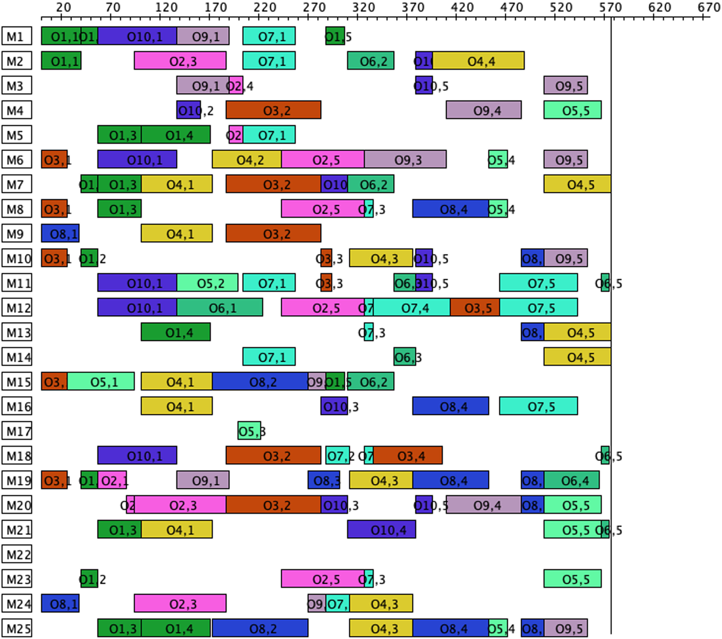
Furthermore, comparing the fitness value results obtained by the same algorithm for the three cooperation ratios, can observe a gradual decrease in the value from a cooperation ratio of 90% to 70%. As per the previous formula, when the cooperative effect is larger, the actual processing time of the job increases, leading to longer completion time and total tardiness, which means that with more skilled worker combinations, the processing time becomes shorter.The grant chart of the best solutions with cooperation ratios of 90%, 80%, and 70% obtained by INSGA-II is shown in Figs. 7 to 9.
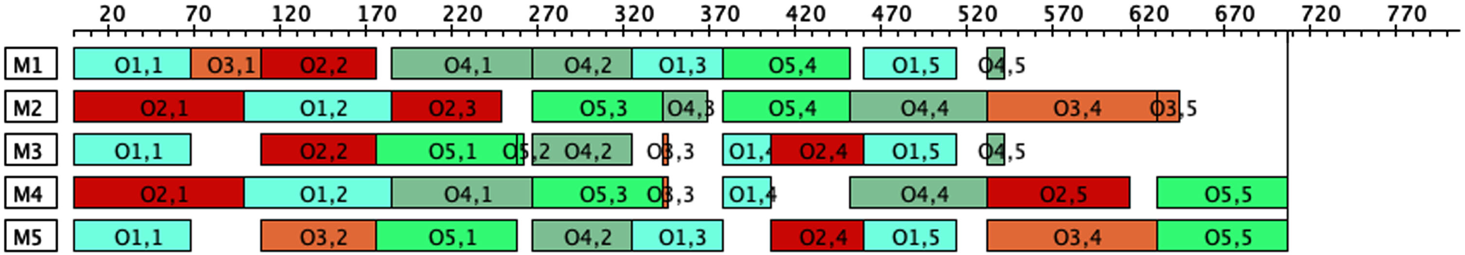
The grant chart of the best solution obtained by INSGA-II when the cooperation ratio is 90%.
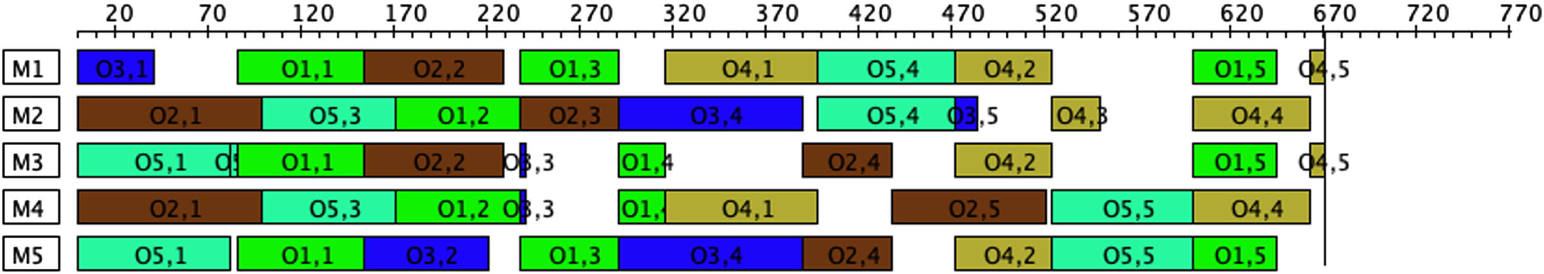
The grant chart of the best solution obtained by INSGA-II when the cooperation ratio is 80%.
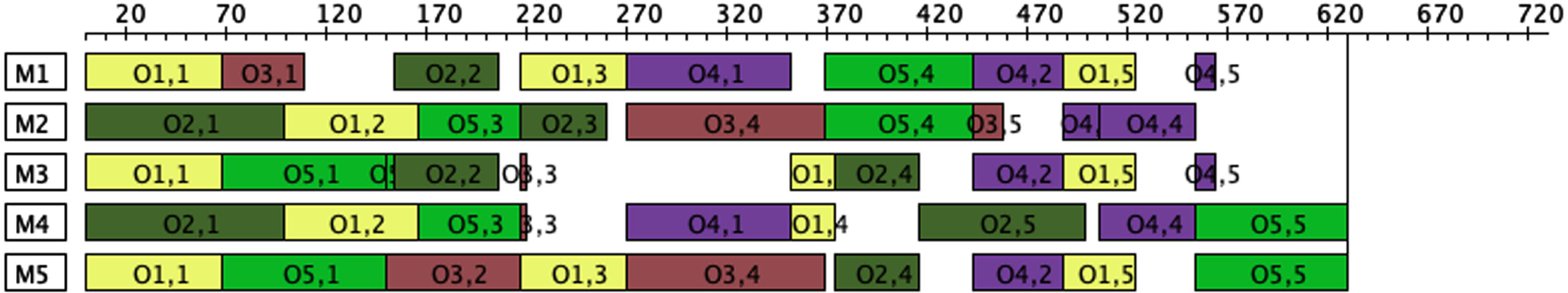
The grant chart of the best solution obtained by INSGA-II when the cooperation ratio is 70%.
Table 13 indicates that at a cooperation ratio of 90%, none of the sets of fitness values obtained by the INSGA-II algorithm are dominated by those obtained by IMOPSO, but all sets of fitness values generate by IMOPSO can be dominated by at least one set of fitness values produced by the INSGA-II algorithm. At a cooperation ratio of 80%, C (IM, IN) and C (IN, IM) are both 0.5, indicating that while both algorithms have one set of fitness value combinations that can be dominated by each other, the INSGA-II algorithm generates significantly more scheduling solutions. Similarly, the effectiveness of the INSGA-II algorithm is demonstrated for a cooperation ratio of 70%.
Comparison between the C values
Note: IM: IMOPSO, IN: INSGA-II.
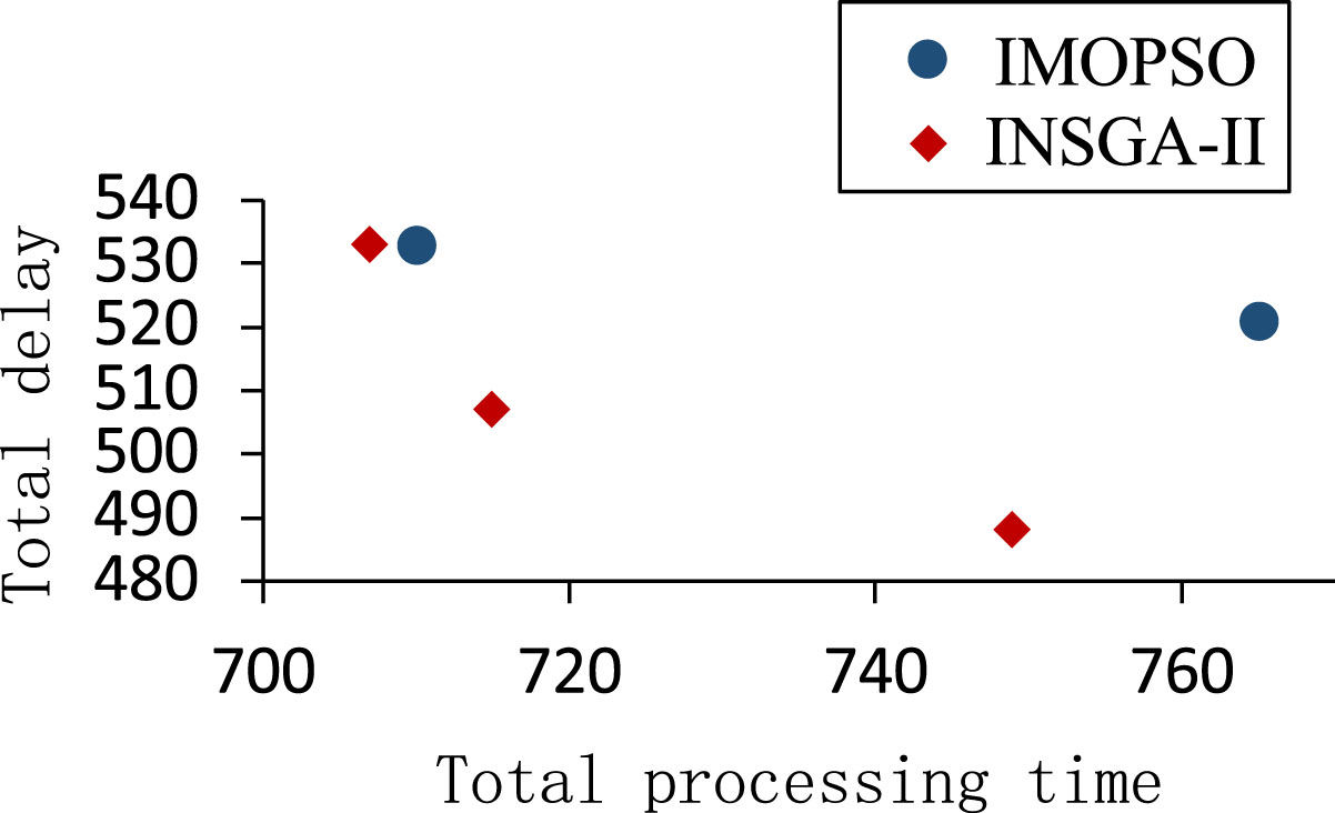
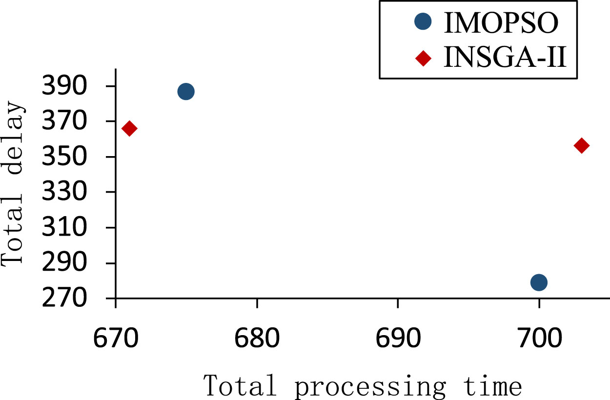
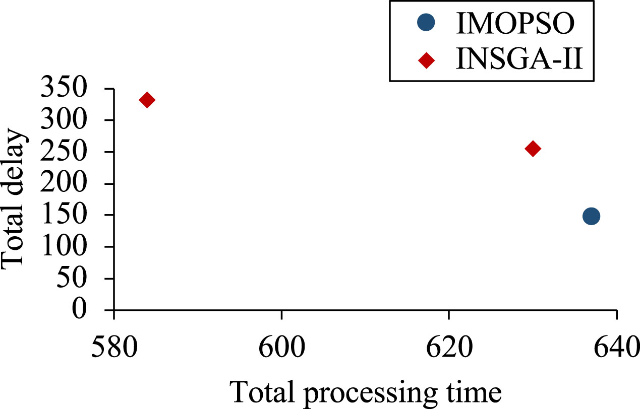
Figures 10 to 12 present scatter plots of the fitness values generated by IMOPSO and INSGA-II at cooperation ratios of 90%, 80%, and 70%, respectively. The plots show that the points representing the INSGA-II algorithm are closer to the bottom left corner of the plot, indicating that the INSGA-II algorithm is more effective and capable of generating relatively better results.
Scatter plots of particle fitness values for IMOPSO and INSGA-II (cooperation ratio is 90%).
Scatter plots of particle fitness values for IMOPSO and INSGA-II (cooperation ratio is 80%).
Scatter plots of particle fitness values for IMOPSO and INSGA-II (cooperation ratio is 70%).
Based on the experimental results, it can be observed that the IMOPSO algorithm generates a relatively small number of scheduling solutions, while the INSGA-II algorithm is capable of generating more solutions. One possible reason for this discrepancy is that the IMOPSO algorithm employs an external population to record better particles, which is currently set to 20 references from previous studies. It is possible that this value may affect the number of particles obtained in the end. On the other hand, the INSGA-II algorithm keeps a certain number of particles in each iteration to enter the next cycle. During the experimental process, it is found that the particles gradually approach the Pareto front during the iteration. However, the final result converges to the same set of fitness values after 200 iterations. When this set of fitness values happens to be the non-dominated solution, a large number of scheduling solutions can be generated.
This paper innovatively considers the cooperative effect into the Multi-objective Hybrid Job-shop Scheduling with Multiprocessor Task problem, proposes a suitable algorithm INSGA-II, and proves the effectiveness of the algorithm as well as the influence of the cooperative effect on the scheduling through simulation experiments, which provides a new perspective and idea for the research of scheduling problems.
We establish a mathematical planning model tailored to this problem and solve it using the improve NSGA-II algorithm, which selects the improved priority operation crossover and adds multiple mutations operation to improve the global search capability and addresses the particle trapped in local optimum problem. Meanwhile, the NSGA-II fast non-dominated sorting and elite retention strategy features are also retained to diversify the optimal solutions obtained.
In the experiments, the INSGA-II algorithm, NSGA-II algorithm, and IMOPSO algorithm are applied to the 5-Job and 10-Job problem cases. When considering cooperation ratios of 90%, 80%, and 70%, the INSGA-II algorithm and IMOPSO algorithm are applied to solve the 5-Job cases, demonstrating the superiority of the INSGA-II algorithm in solving problem with both objectives and calculating multiple efficient scheduling solutions.
In future research, alternative solution objectives will be considered based on realistic conditions to better match the current operational requirements of discrete manufacturing enterprises. Additionally, further algorithm improvements will be explored to address the research problem more effectively and efficiently, and generate diverse and satisfactory scheduling solutions that enhance enterprise efficiency.
Footnotes
Acknowledgment
This work was supported by Humanities and Social Sciences Foundation of the Ministry of Education of China (No. 21YJA630012), the Fundamental Research Funds for the Central Universities (No. 2023SKY06).