Chaotic fuzzy iterated function systems

Abstract

It is observed that IFSs are defined based on the concept that the iterates take only an integer number of times. This work studies the dynamics of functions, where a function can iterate r times for every r ∈ R. Utilizing concepts from fuzzy sets, r-times iterates of a function are defined for r ∈ R. The study demonstrates that the chaotic property can be generalized to this new iterative concept. The chaotic behavior of a function is then extended using this iterative concept.

Keywords

Iterated function systems fuzzy functions chaotic functions

1 Introduction

John Hutchinson [13] set up a theory of Iterated Function System(IFS) in 1981. Benoit Mandelbrot [18] popularized the theory by introducing fractals as an attractor of an IFS. Michael Barnsley and others [4] showed that if the contraction of an IFS depends continuously on parameters, then the corresponding attractor also depends continuously on the respective parameter with respect to the Hausdorff metric. The theory of Infinite Iterated Function systems(IIFS) of a countably infinite number of contractive mappings was developed by H.Fernau [12]. Hausdorff and packing measures of the Conformal Iterated Function System(CIFS) were discussed in [6]. The topological pressure of the limit set of parabolic IFS (PIFS) was studied in [7]. Alexandru Mihail [20] generalized IFS to Recurrent IFS(RIFS). Generalized countable IFS (GCIFS) are contractions from X × X to X instead of contractions on the metric space X to itself. It was proved [1] that if all the contractions of GCIFS are Lipschitz with respect to a parameter then the associated attractor depends continuously on the respective parameter. Real Projective IFS(RPIFS) was studied by Barnsley and A. Vince [5]. A topological Version of IFS was studied by Alexandru Mihail [19]. A study of the Topological Version of IIFS was initiated by Dan Dumitru et. al[10]. A. Vince characterized Mobius IFS that possessing an attractor. Another approach to the study of the Topological Version of IFS is due to K. Lesnaik [16, 17]. Detailed discussion on IFS can be seen in, [9, 21].

An Iterated function system is viewed as a dynamical system when the set of function become singleton. Generally, a dynamical system is a tuple (T, X, f), where T is a monoid, X is a nonempty empty set and f is a function, f : T × X → X . In 1965 Zedech [23] introduced Fuzzy sets. And the fuzzy dynamical system was systematically introduced in 1973 by Nazaroff [22]. But the time-dependent dynamical system was explicitly defined by Kloeden in 1980 [14]. He defined a Fuzzy dynamical system(FDS) on a state space X, axiomatically in terms of a fuzzy attainability set mapping $F : X \times T \to C$ . Where $C$ denotes the collection of nonempty compact fuzzy subsets of X. A study of the Fuzzy version of IFS was initiated by Alexandru Mihail [19] by considering the attractor of an IFS as a certain fuzzy set. A Different approach to fuzzy IFS was carried out in [11]. The Fuzzy iterated Function System is defined so far in [2] as ${(D^{n}, d_{\infty}); f_{i} : D^{n} \to D^{n}, i = 1, 2, . . ., m}$ where $D^{n}$ is the space of fuzzy sets of $R^{n}$ .The concept of Fuzzy Chaotic Systems was first introduced by Zhong Li in 2006 [24]. Nevertheless, our approach to constructing a Fuzzy Iterated Function System and exploring chaotic properties differs significantly, especially in the context of function iterates

As it is known that a function defined on a set can compose itself many times, The resulting function is called an Iterated function. But the arising question is " Why do we take the composition only n times, where n is an integer?" And we know that fⁿ denotes the function obtained by taking n times the composition of the function f. Then how can we define f^r, when r is a non-integer number? In this paper, we define iterated functions got by iterating a function not merely n times but also r times, where n is an integer and r is a real number. Then we study the chaotic behavior of a function using these distorted Iterated functions in support of evidently defined fⁿs. This approach generalizes IFS in terms of iterations.

Consider that non-integer time iterations often encompass the utilization of advanced mathematical principles and techniques, encompassing fractal calculus, special functions, and complex analysis. These notions hold particular relevance within scenarios characterized by the existence of continuous or fractional patterns, in contrast to discrete steps. Such concepts play a role in enhancing the depth of understanding of complex systems and phenomena.

2 Preliminaries

Definition 2.1. [IFS][19] An Iterated Function System on a metric space (X, d) consists in a family of contractions $(f_{k})_{k = \bar{1, n}}$ on X and it is denoted by $S = ((X, d), (f_{k})_{k = \bar{1, n}})$

Definition 2.2. [Topological Transitivity][8] A function f : S → S is said to be topological Transitive if for any pair of nonempty open sets U and V in S there is an integer k > 0 such that f^k (U) ∩ V is nonempty.

Definition 2.3. [Periodic Points][8]A point x ∈ X is a periodic point with prime period n of a function f : X → X if n is the least integer such that fⁿ (x) = x.

Definition 2.4. [Sensitive dependence on initial conditions][8] f : J → J has sensitive dependence on initial conditions if there exists a δ > 0 such that, for any x ∈ J and any neighbourhood N of x, there exists y ∈ N and n ≥ 0 such that |fⁿ (x) - fⁿ (y) | > δ.

Definition 2.5. [Fuzzy Set][15]If X is a collection of objects denoted by x, then a fuzzy set A in X is a set of ordered pairs: A= {(x, M_A (x)) : x ∈ X}. M_A (x)is called the membership function or grade of membership of x in A that maps X to the closed interval [0, 1].

Definition 2.6. [Support of a Fuzzy Set][15]The support of a fuzzy set A, S (A) = {x ∈ X : M_A (x) >0}

Fuzzy functions can be classified into the following three, according to which aspect of the crisp function the fuzzy concept was applied.

Crisp functions with fuzzy constraints

Crisp function which propagates the fuzziness of independent variable.

function that is itself fuzzy, the fuzzifying function blurs the image of the crisp independent variable.

Using the Third type of fuzziness define the fuzzy function as,

Definition 2.7. [Fuzzy Functions][15]Let X, and Y are two non-empty sets. Then $f : X \to F (Y)$ is called a Fuzzy function from X to Y.

3 Fuzzy Iterated Function System

Consider a function f from a set X to the set of fuzzy sets on X, denoted as $F (X)$ . In this context, the images of the elements under f, represented as f (x), are fuzzy sets defined on the set X. This concept of a "fuzzy function" is employed to define an iterated function that is applied a number of times corresponding to each real number r in the set R. To ensure the completeness of this process, it is imperative that every element in X has a corresponding image.

In the scenario where the membership value of the fuzzy set representing the image of an element is non-zero, we have the flexibility to select an element from the support of that fuzzy set as an image, if deemed necessary. As such, we designate a function as a "fuzzy function" if it adheres to the property outlined in the following definition.

Definition 3.1. [Fuzzy Function on X] Let X be a nonempty set and $F (X)$ be the fuzzy power set of X. Then $f : X \to F (X)$ is called a fuzzy function if for every x ∈ X the support of f (x), S (f (x)) ≠ φ.

3.1 Fuzzy Iteration of a function

Typically, the concept of iterating a function is applied for integer values of time. However, instead of restricting the iteration of the function f to integer values of time, we propose to define the iteration of f for real values of time, denoted as r.

Definition 3.2. [r^th iterate of f] Consider a non-empty set X, and let f : X → X be a bijection on X. Then, for every r ∈ R, the r^th iterate of f, denoted as f^r, is a fuzzy function defined on X, which complies with the following conditions:

If ∃y ∈ Xsuch that, the membership value of y in the fuzzy set f^r (x), M_f^r(x) (y) =1 then M_f^r(x) (p) ≠1 for every p ≠ y, p ∈ X

The membership value of the element f^k (x) in the fuzzy set f^k (x), M_f^k(x) (f^k (x)) =1 for every k ∈ Z.

The values of f^k (x) are known for all k in the set of integers Z. The following example represents one of the r^th iterations of f, defining f^r (x) using the known values f^k (x).

Throughout this paper, we use the notation f^r (x, y) to denote the membership value of the element y ∈ X in the fuzzy set f^r (x).

Example 3.1. Let f : R → R is a bijective function. Define r^th iterate of f as, $f^{r} (x, y) = \frac{1}{e^{d (f^{⌊ r ⌋} (x), y)}} (∣ \cos (2 π r) ∣) .$

Example 3.2. Let (X, d) be a metric space and f : X → X is a bijection on X. Define r^th iterates of f as, $f^{r} (x, y) = \frac{(\frac{1}{e^{d (f^{⌊ r ⌋} (x), y)}} + \frac{1}{e^{d (f^{⌈ r ⌉} (x), y)}})}{2} .$

Definition 3.3. [Fuzzy Iterated Function System(FIFS)] A Fuzzy iterated Function System on a metric space (X, d) consists a bijective function f defined on X and an iterative method f^r, r ∈ R. And it is denoted by S = (X, f, f^r)

From the definition, it is clear that we can define more than one type of r-times iteration method for the same function and space.

Example 3.3. Consider R with the usual metric d on it, and f : R → R defined as f (x) =2x. Then,

fⁿ (x) =2ⁿx.

Define $f^{r} (x, y) = \frac{(\frac{1}{e^{d (f^{⌊ r ⌋} (x), y)}} + \frac{1}{e^{d (f^{⌈ r ⌉} (x), y)}})}{2} .$ Then (X, f, f^r) is a FIFS.

In this example the membership value of f^r (x) is highest for the points that are nearest to the points f^m (x) and fⁿ (x), where m =⌊ r ⌋, the largest integer less than or equal to r and n =⌈ r ⌉, the smallest integer greater than or equal to r. Graph of the images of 3 under the functions f³, f^2.64, f^3.7 and f^0.7 are given in Fig. 1.

Fig. 1

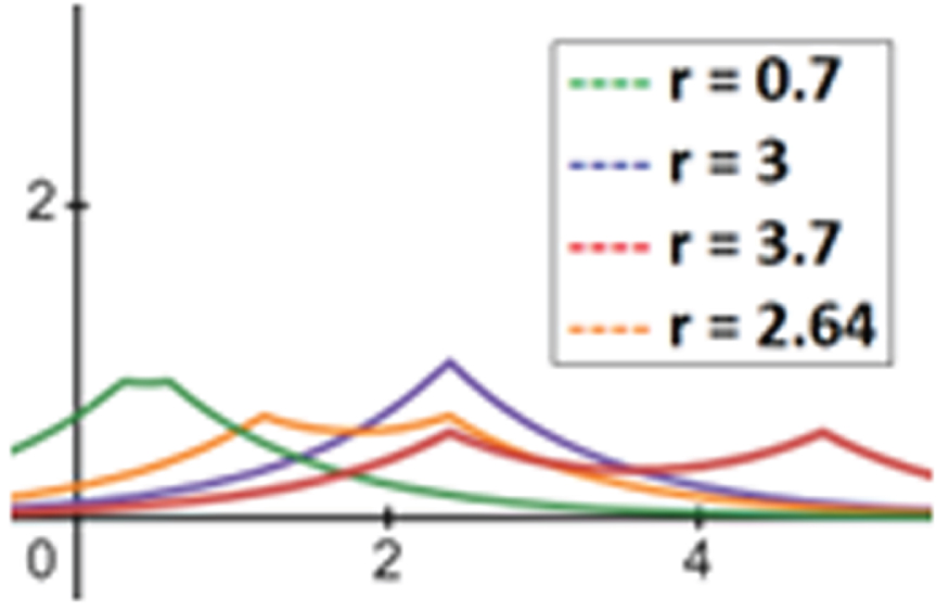
f^r (3) for different values of r

Example 3.4. Let X = [0, 1] with usual metric on it, and g : X → X defined as g (x) = x² define $g^{r} (x, y) = \frac{1}{e^{d (g^{⌊ r ⌋} (x), y)}} (∣ \cos (2 π r) ∣)$ . Then (X, g, g^r) is an FIFS.

Graph of the images of 0.5 under the functions g³, g^2.64, g^3.7 and g^0.7 are given in Fig. 2.

Fig. 2

g^r (3) for different values of r

Fig. 3

Original image

Example 3.5. Let $X = C^{\infty} [R]$ , the set of all infinitely differentiable functions on R, with $d (f, g) = sup_{x \in R} | f (x) - g (x) |$ defining the supremum metric on X. Additionally, let D : X → X be defined as $D (f) = \frac{df}{dx}$ . Now, we define D^r (f) as a fuzzy function on X: the membership value of g ∈ X in the fuzzy set D^r (f) is given by $D^{r} (f, g) = \frac{\frac{1}{e^{d (D^{⌊ r ⌋} (f), g)}} + \frac{1}{e^{d (D^{⌈ r ⌉} (f), g)}}}{2}$ . Therefore, (X, D, D^r) forms a Fuzzy Iterated Function System.

Note that when we defuzzify the fuzzy set D^r (f) using the height method(defuzzify f^r (x) to the point y with maximum membership value(If there is more than one such point, choose one of them randomly.), we obtain a single function defined on R. This can be interpreted as a fractional derivative of f.

Fig. 4

Iterations of the image up to 10th iteration

Example 3.6. Let X be the space of all m × m pixel images, where each pixel represents a single point in the image. The pixel values in a grayscale image typically range from 0 to 255, where 0 represents black, 255 represents white, and values in between represent varying shades of gray. Define f : X → X as the ij^th pixels value of image f (A), of an image A is

f (A) _ij = ${\begin{matrix} (A)_{ij}^{2} & if \sqrt{{(\frac{\partial I}{\partial x})}^{2} + {(\frac{\partial I}{\partial y})}^{2}} > \frac{225}{n + 1} \\ (A)_{ij} & otherwise \end{matrix}$ .

I (x, y) is the gray scale value. function. Now, define $f^{r} (A, B) = \frac{\frac{1}{e^{d (f^{⌊ r ⌋} (A), B)}} + \frac{1}{e^{d (f^{⌈ r ⌉} (A), B)}}}{2}$ . Then (X, f, f^r) is a Fuzzy Iterated Function System.

We are transforming an image by detecting its edges through the computation of intensity gradients. The process involves identifying areas where the intensity undergoes rapid changes, effectively highlighting edges within the image. The reference to "Fig. 3" signifies the original image under consideration. Despite the inherent challenge posed by the low contrast in the original image, the iterative application of the edge detection process consistently improves the delineation of edges. But, applying the Canny edge detection method to low-contrast images often leads to a complete blackout, where the entire image appears dark.

Examine Figure4. With each round of the process, the edges become clearer, but at the same time, the noise also increases. To tackle this, our fuzzy iteration method helps by incorporating intermediate steps. This helps strike a good balance between making the edges stand out and controlling unwanted noise in the image processing. Fig. 5 displays the result after the 9.5th iteration.

Fig. 5

Iteration 9.5

This scenario is an example of a situation where fuzzy iterations prove advantageous.

The algorithm for find the r^th iterated image is given in algorithm 1

Agorithm 1 Compute r^th iterated image

Initialize m1 = floor (r) and m2 = ceil (r) based on r

Create an empty final _ image matrix with the same shape as images [m1]

for x in range(final_image.shape[0]) do

for y in range(final_image.shape[1]) do

Compute gradient _ image using compute_gradient on images [m1]

Check if gradient magnitude at (x, y) is $\geq \frac{225}{r}$

if gradient magnitude condition is met them

Create s _ values ranging from 0 to 225 with step 1

for each s in s _ values do

Calculate

$ir = \frac{\frac{1}{e^{d (f^{⌊ r ⌋} (A), B)}} + \frac{1}{e^{d (f^{⌈ r ⌉} (A), B)}}}{2}$

end for

Assign intensity value corresponding to the maximum ir to final _ image [x, y]

else

Assign pixel value from images [m1] to final _ image [x, y]

end if

end for

Return final _ image

3.2 Chaos in FIFS

In the study of the dynamics of a function, various conditions exist to determine when a function can be considered chaotic.

Definition 3.4. [Chaotic function][5] Let (X,d) be a metric space. A continuous function f : X → X is said to be chaotic if

f is Topologically transitive. and,

Set of periodic points of f is dense in X.

Both of these aspects rely on the iteration of the specified function. Therefore, in accordance with the newly introduced iterative method in definition 3.2, we establish an alternative perspective for defining chaotic functions.

Suppose we have a function f defined on a metric space X that exhibits topological transitivity. In such a case, for any open sets U and V within X, there exists an n in the set of natural numbers N such that the intersection of fⁿ (U) and V is non-empty (i.e., fⁿ (U) ∩ V ≠ φ). This implies the existence of u in U and v inV, such that fⁿ (u) = v, and we can express this relationship as fⁿ (u, v) =1. Consequently, we can introduce the concept of ϵ-Topological Transitivity as described below.

Definition 3.5. [ϵ-Topological transitivity] Let X be a metric space, f : X → X is a bijection, and ϵ ∈ (0, 1]. Then f is considered ϵ-topologically transitive in the system (X, f, f^r) if, for every pair of open sets U and V in X, there exists r ∈ R (the set of real numbers), u ∈ U, and v ∈ V such that f^r (u, v) ≥ ϵ .

Example 3.7. Let S¹ denote the unit circle in the plane. We denote a point in S¹ by its angle measured in radians in the standard manner. Hence a point is determined by any angle of the form θ + 2kπ for an integer k. Thus we can consider S¹ = {θ|0 < θ ≤ 2π} and define metric d (θ₁, θ₂) = |θ₁ - θ₂|.

Now let f (θ) = ${\begin{matrix} 2 θ & 0 < θ \leq π \\ 2 π - 2 θ & π < θ < 2 π \end{matrix}$ defined on S¹. Define $f^{r} (θ, φ) = \frac{(\frac{1}{e^{d (f^{⌊ r ⌋} (θ), φ)}} + \frac{1}{e^{d (f^{⌈ r ⌉} (θ), φ)}})}{2} .$ Then f is ϵ- topological transitive ∀ϵ ∈ (0, 1]

We know that f is topologically transitive. This implies that for any pair of open sets U and V in the space S¹, there exists an integer n such that fⁿ (U)∩ V ≠ ∅. This condition implies the existence of elements φ in U and θ in V such that fⁿ (φ) = θ

⇒fⁿ (φ, θ) =1. Consequently, for every ϵ in the interval (0, 1], we have fⁿ (φ, θ) ≥ ϵ.

Hence, in the dynamical system (S¹, 2θ, f^r), it follows that f is ϵ-topologically transitive for every ϵ ∈ (0, 1].

We promptly obtain a result that,

Theorem 3.1. If a bijective function f : X → X, defined on a metric space X, is topologically transitive, then f is ϵ-topologically transitive for every ϵ ∈ (0, 1] in every FIFS (X, f, f^r), but not vice versa. Proof. Let U and V be two arbitrary open sets of X. Since f is topologically transitive ∃k ∈ Z such that f^k (U) ∩ V ≠ φ .

⇒ ∃ u ∈ U, v ∈ V such that f^k (u) = v⇒f^k (u, v) =1⇒f^k (u, v) ≥ ϵ, ∀ ϵ ∈ [0, 1]

⇒f is ϵ-topologically transitive.

Example 3.8. Let f : S¹ → S¹ be defined by

$f (θ) = θ + \frac{π}{8}$ . Using the same iterative method f^r as described in example 3.7, we can conclude that f^r is $\frac{1}{2}$ -topologically transitive but not topologically transitive. The distance between any two open sets U and V is at least 2π, and the distance between any f^k (φ) and f^k+1 (φ) is $\frac{π}{8}$ for every k in Z. This implies that there exists an r in R such that . If we choose $ϵ = \frac{1}{2}$ , then f^r (φ, θ) ≥ ϵ for an r in the interval (k, k + 1). This implies that f is ϵ-topologically transitive.

This is an example of functions that are ϵ-topologically transitive but not topologically transitive.

In this example, we can see that the value ϵ of an ϵ-topologically transitive function depends on the distance between the sets fⁿ (U) and the set V. The distance is equal to 0 for an n means ϵ = 1, that is, f is 1- topological transitive. As per the distance increase ϵ decreases.

Example 3.9. The function f (x) = x (1 - x) defined on [0, 1] is $\frac{1}{e} -$ Topologically transitive in the system ([0, 1] , f, f^r), where

$f^{r} (x, y) = \frac{(\frac{1}{e^{d (f^{⌊ r ⌋} (x), y)}} + \frac{1}{e^{d (f^{⌈ r ⌉} (x), y)}})}{2}$ Here it is clear that the distance between any subset of [0, 1] and the range of f is at most 1. There fore f is $\frac{1}{e} -$ Topologically transitive.

Theorem 3.2. In the system (X, f, f^r) where $f^{r} (x, y) = \frac{(\frac{1}{e^{d (f^{⌊ r ⌋} (x), y)}} + \frac{1}{e^{d (f^{⌈ r ⌉} (x), y)}})}{2},$ f is topologically transitive iff f is ϵ-topologically transitive, when ϵ = 1. Proof. f is topologically transitive implies for any pair of open sets U and V, ∃k ∈ Z such that

f^k (U) ∩ (V) ≠ φ

⇒ ∃ u ∈ U and v ∈ V such that $f^{k} (u) = v \Rightarrow f^{k} (u, v) = \frac{(\frac{1}{e^{d (f^{⌊ k ⌋} (u), v)}} + \frac{1}{e^{d (f^{⌈ k ⌉} (u), v)}})}{2} = 1$

⇒ f^k (u, v) =1 for a u ∈ U and v ∈ V

⇒ f is 1-topologically transitive.

Conversely, assume that f is 1-topologically transitive. This implies that for every pair of open sets U and V, there exists r ∈ R, u ∈ U, and v ∈ V such that f^r (u, v) =1. Let k be the integer such that r ∈ [k, k + 1]. There are two cases:

r ∈ (k, k + 1).r ∈ I

r ∈ I

case 1: r ∈ (k, k + 1). Then f^r (u, v) =1

$\Rightarrow \frac{\frac{1}{e^{d (f^{k} (u), v)}} + \frac{1}{e^{d (f^{k + 1} (u), v)}})}{2} = 1$ .

$\Rightarrow \frac{1}{e^{d (f^{k} (u), v)}} = 1$ and $\frac{1}{e^{d (f^{k + 1} (u), v)}} = 1$ , since the maximum value for $\frac{1}{e^{| x |}}$ is 1.

case 2: r ∈ I. then ⌊r ⌋ = ⌈ r ⌉ = r. Then f^r (u, v) =1

$\Rightarrow \frac{\frac{1}{e^{d (f^{r} (u), v)}} + \frac{1}{e^{d (f^{r} (u), v)}})}{2} = 1 \Rightarrow \frac{1}{e^{d (f^{r} (u), v)}} = 1$ .

In either case we get, $\frac{1}{e^{d (f^{k} (u), v)}} = 1 .$ Which implies d (f^k (u) , v) =0 ⇒f^k (u) = v .

(If k is a negative integer, act f^-k on both sides.) So we get that ∃ k ∈ Z such that f^k (U) ∩ V ≠ φ.

Hence the proof.

Next, we define periodic points from the perspective of the r-times iterations.

Definition 3.6. [ϵ-Periodic Point] A point x ∈ X is said to be an ϵ-periodic point of a bijective function, f : X → X in the system (X, f, f^r) if there exist r ∈ R such that f^r (x, x) = ϵ .

Example 3.10. Let (X, f, f^r) be the system defined as X = [0, 1], f : X → X defined as f (x) = x² and $f^{r} (x, y) = \frac{(\frac{1}{e^{d (f^{⌊ r ⌋} (x), y)}} + \frac{1}{e^{d (f^{⌈ r ⌉} (x), y)}})}{2} .$ . Then every point in X is α- periodic points, for $α > \frac{1}{e}$ . Here, the distance between x and fⁿ (x) is 1 at the maximum. Thus the membership value $f^{r} (x, y) > \frac{1}{e}$ ∀x, y ∈ X. Therefore every point is an α- periodic points, for $α > \frac{1}{e}$ .

In this example, it is evident that as the distance between x and fⁿ (x) diminishes, the point x transforms into an ϵ-periodic point, with ϵ approaching closer to 1.

Proposition 3.1. In the system (X, f, f^r), x is a 1-periodic point ⇔ x is a periodic point.

Definition 3.7. [ϵ-Chaotic Functions] Let X be a metric space and ϵ ∈ [0, 1] , f : X → X is said to be an ϵ-chaotic function in the system(X, f, f^r) if,

f is ϵ-Topologically transitive.

Set of α-Periodic point, α ≥ ϵ is dense in X.

Example 3.11. Let f : S¹ → S¹ defined by

$f (θ) = θ + \frac{π}{8}$ is $\frac{1}{2} -$ Chaotic in (S¹, f, f^r), where $f^{r} (x, y) = \frac{(\frac{1}{e^{d (f^{⌊ r ⌋} (x), y)}} + \frac{1}{e^{d (f^{⌈ r ⌉} (x), y)}})}{2}$

Example 3.12. Consider R with discrete metric and for f : R → R let $f^{r} (x, y) = \frac{(\frac{1}{a^{d (f^{⌊ r ⌋} (x), y)}} + \frac{1}{a^{d (f^{⌈ r ⌉} (x), y)}})}{2}$ , a ≠ 0 . Then, f is $\frac{1 + a}{2 a} -$ chaotic if a ∈ (0, 1] and $\frac{1}{a} -$ topologically transitive if a ∈ (- ∞ , 0) ∪ (1, ∞) . in the system(X, f, f^r)

Example 3.13. Consider R with discrete metric, let $f^{r} (x, y) = \frac{(\frac{1}{e^{d (f^{⌊ r ⌋} (x), y)}} + \frac{1}{e^{d (f^{⌈ r ⌉} (x), y)}})}{2} .$ Then the identity function f (x) = x is $\frac{1}{e} -$ chaotic.

We get that in some FIFSs the chaotic and 1-chaotic properties are equivalent. What are the common characteristics of such systems? In order to determine this, we require the following definitions.

Definition 3.8. [(x, y) _α] Let (X, f, f^r) be an FIFS and (x, y) ∈ X × X. Then for α ∈ [0, 1] define, (x, y) _α = {r ∈ R∣f^r (x, y) = α} .

Proposition 3.2. Let x, y ∈ X then

(x, y) _p ∩ (x, y) _q = φ, ∀p ≠ q ∈ [0, 1].

Proof. Suppose that ∃ (x, y) ∈ X × X and p ≠ q ∈ [0, 1] such that (x, y) _p ∩ (x, y) _q = φ . Which implies ∃r ∈ (x, y) _p ∩ (x, y) _q⇒f^r (x, y) = q and f^r (x, y) = p⇒p = q it is a contradiction.

Proposition 3.3. (u, v) ₁ ∩ (v, w) ₁ = φ, ∀v ≠ w .

Theorem 3.3. If for an FIFS (X, f, f^r) the (u, v) ₁s are subsets of Z for every pair (u, v) ∈ X × X then, f is 1-chaotic if and only if f is chaotic.

Proof. Assume that f is Chaotic. Then f is Topologically transitive and periodic points of f are dense in X.

⇒f is 1-topologically transitive and 1-periodic points are dense in X.

⇒f is 1-topologically transitive and 1-periodic points are dense in X

⇒ f is 1-chaotic.

Conversely, assume that f is 1-chaotic. This implies f is 1-topological transitive and 1-periodic points are dense in X.

Let U,V be two arbitrary open sets in X.

f is 1-topological transitive

⇒ ∃ r ∈ R, u ∈ U and v ∈ V such that f^r (u, v) =1⇒r ∈ (u, v) ₁.

(u, v) ₁ ⊂ Z for every (u,v) ⇒r = k ∈ Z.

By the properties of f^r, f^k (u, f^k (u)) =1 and f^k (u, v) =1. Which implies f^k (u) = v . ⇒f^k (U) ∩ V ≠ φ⇒ f is topologically transitive.

Now, let x be a 1-periodic point. This ⇒ ∃r ∈ R such that f^r (x, x) =1⇒r ∈ (x, x) ₁⇒r = k ∈ I. f^k (x, f^k (x)) =1, f^k (x, x) =1⇒f^k (x) = x⇒x is a periodic point. Hence periodic points are dense in X. So, the proof is here.

Theorem 3.4. In the system (X, f, f^r) where $f^{r} (x, y) = \frac{1}{e^{d (f^{⌊ r ⌋} (x), y)}} ∣ \cos π r ∣,$ f is topologically transitive iff f is ϵ-topologically transitive, for ϵ = 1.

Proof. Suppose that f is topologically transitive.

⇒ for every pair of open sets U and V

∃k ∈ Z, u ∈ U and v ∈ V such that f^k (u) = v. Then $f^{k} (u, v) = \frac{1}{e^{d (f^{⌊ k ⌋} (u), v)}} ∣ \cos π r ∣ = 1$

⇒ f is 1-topologically transitive.

Conversely, assume that f is 1-topologically transitive.

⇒ for every open sets U and V ∃r ∈ R, u ∈ U and v ∈ V, such that f^r (u, v) =1

$\Rightarrow \frac{1}{e^{d (f^{⌊ r ⌋} (u), v)}} | \cos π r ∣ = 1$

⇔|cosπr∣ = e^{d(f^⌊r⌋(u),v)} ⇔ ∣cosπr∣ = e^{d(f^⌊r⌋(u),v)} = 1

⇔r ∈ I and f^⌊r⌋ (u) = f^r (u) = v ⇒f^r (U) ∩ V ≠ φ

⇒f is topologically transitive.

Theorem 3.5. Let (X, d) be a metric space and

$f^{r} (x, y) = \frac{(\frac{1}{e^{d (f^{⌊ r ⌋} (x), y)}} + \frac{1}{e^{d (f^{⌈ r ⌉} (x), y)}})}{2},$ Then f is 1-chaotic in the system (X, f, f^r) iff f is chaotic.

Proof. Suppose that f is chaotic. Then f is topologically transitive and the set of periodic points of f is dense in X.

From theorem 3.2 we get, f is 1-topologically transitive

⇔ f is topologically transitive. (1)

Now we will prove that x is a 1-periodic point if and only if x is a periodic point.

Let x be a periodic point of f. Which implies that

∃k ∈ Z such that f^k (x) = x. Let r = k then, $f^{r} (x, x) = \frac{(\frac{1}{e^{d (f^{⌊ r ⌋} (x), x)}} + \frac{1}{e^{d (f^{⌈ r ⌉} (x), x)}})}{2} = 1$

⇒ x is a 1-periodic point.

Conversely, Let x be a 1-periodic point. Then ∃r ∈ R such that f^r (x, x) =1.

case 1: r ∉ Z, then

$f^{r} (x, x) = \frac{(\frac{1}{e^{d (f^{⌊ r ⌋} (x), x)}} + \frac{1}{e^{d (f^{⌈ r ⌉} (x), x)}})}{2}$ = 1

⇒ $\frac{(\frac{1}{e^{d (f^{k} (x), x)}} + \frac{1}{e^{d (f^{k + 1} (x), x)}})}{2} = 1,$ where k =⌊ r ⌋, and k+ 1 = ⌈ r ⌉.

⇒ d (f^k (x) , x) and d (f^k+1 (x) , x) are equal to 0

⇒f^k (x) = f^k+1 (x) = x

⇒x is a fixed point.

case 2: r ∈ Z, then

$f^{r} (x, x) = \frac{(\frac{1}{e^{d (f^{r} (x), x)}} + \frac{1}{e^{d (f^{r} (x), x)}})}{2}$ = 1

⇒f^r (x) = x . r ∈ Z ⇒ x is a periodic point.

So, in either case, x is a 1-periodic point if and only if x is a periodic point.(2)

Now (1) and (2) give the proof.

4 Sensitive dependence on initial conditions

Sensitive dependence on initial conditions is a concept in chaos theory that describes how small differences in the initial conditions of a dynamical system can lead to significantly different outcomes over time. In chaotic systems, even a tiny change in the starting point can result in a vastly different trajectory. Here we generalize the definition of sensitive dependence on initial conditions to the existence of a real number r such that images of x and y, obtained by defuzzifying the f^r (x) and f^r (y), are separated by at least the distance δ.

In this section, we use η_x to denote the collection of all neighborhoods of x in the metric space X.

Definition 4.1. Let (X, f, f^r) be a FIFS. f has sensitive dependence on initial conditions in FIFS if ∃δ > 0 such that for every x ∈ x and a neighborhood N_x of x, ∃y ∈ N_x and r ∈ R such that $d (p_{x}^{r}, p_{y}^{r}) \geq δ$ , where $p_{x}^{r}, p_{y}^{r} inX$ such that $f^{r} (x, p_{x}^{r}) = h (f^{r} (x))$ and $f^{r} (y, p_{y}^{r}) = h (f^{r} (y))$ . Where h (f^r (x)) denotes the height of the fuzzy set f^r (x).

Proposition 4.1. If f has sensitive dependence on initial conditions then f has sensitive dependence on initial conditions on FIFS.

Proof. Suppose that ∃δ > 0 such that ∀x ∈ X and neighborhood N_x of x, ∃y ∈ N_x and k ∈ I such that d (f^k (x) , f^k (y)) > δ.

Let x ∈ X arbitrary and N_x is an arbitrary neighborhood of x. Then ∃y ∈ N_x and k ∈ I such that d (f^k (x) , f^k (y)) > δ.

We have f^k (x, f^k (x)) =1 and f^k (y, f^k (y)) =1. Take $p_{x}^{k} = f^{k} (x)$ and $p_{y}^{k} = f^{k} (y)$ .

Then $d (p_{x}^{k}, p_{y}^{k}) = d (f^{k} (x), f^{k} (y)) > δ$

Hence the proof.

Proposition 4.2. The converse of the above result is not true.

Example 4.1. Consider the system (S¹, f, f^r) where f : S¹ → S¹ defined as f (θ) = θ + 2πλ, λ ∈ Q^c. Then f does not satisfy the condition of sensitive dependence on initial conditions. But it satisfies the condition of sensitive dependence on initial conditions in (S¹, f, f^r). Where f^r (x, y) is defined as $f^{r} (x, y) = {\begin{matrix} \frac{1}{e^{d (f^{⌊ r ⌋} (x), y)}} | \cos 2 π r ∣, & r \in I \\ \frac{1}{e^{d (f^{⌊ rx ⌋} (x), y)}} ∣ \cos 2 π r ∣, & r \in I^{c} \end{matrix}$

Proof. Let x ∈ X, N ∈ η_x and y ∈ N. And let d (x, y) = ϵ. Choose r ∈ I^c very large such that ⌊rx⌋ and ⌊ry⌋ are not equal so that

∣2πλ (⌊ rx ⌋ - ⌊ ry ⌋) ∣ ≥ δ + ϵ . $f^{r} (x, z) = \frac{1}{e^{d (f^{⌊ rx ⌋} (x), z)}} ∣ \cos 2 π r ∣$ and

$f^{r} (y, z) = \frac{1}{e^{d (f^{⌊ ry ⌋} (y), z)}} ∣ \cos 2 π r ∣$ .

Supremum of f^r (x, z) and f^r (y, z) attains at f^⌊rx⌋ (x) and f^⌊ry⌋ (y) respectively.

⇒ $\begin{matrix} ∣ p_{x}^{r} - p_{y}^{r} ∣ & = ∣ f^{⌊ rx ⌋} (x) - f^{⌊ ry ⌋} (y) ∣ \\ = ∣ x + ⌊ rx ⌋ 2 π λ - y - ⌊ ry ⌋ 2 π λ ∣ \\ \geq - ∣ x - y ∣ + ∣ 2 π λ (⌊ rx ⌋ - ⌊ ry ⌋) ∣ \\ = ∣ 2 π λ (⌊ rx ⌋ - ⌊ ry ⌋) ∣ - ϵ \\ \geq δ + ϵ - ϵ \\ \geq δ \end{matrix}$

Hence the proof.

Theorem 4.1. A function f defined on the FIFS S has sensitive dependence on initial conditions. If the S satisfies the conditions

The functions h_x : R → [0, 1] defined as h_x (r) = h (f^r (x)) is an increasing onto map, ∀x ∈ X

∀r ∈ R, the functions g_r : X → X defined as $g_{r} (x) = p_{x}^{r}$ is metric differentiable and H_x : R → R defined by $H_{x} (r) = g_{r}^{'} (x)$ is an increasing function.

Then f satisfies the condition of sensitive dependence on initial conditions.

Proof. Assume that f has sensitive dependence on initial conditions on S.Thus ∃δ > 0 such that ∀x ∈ X and N ∈ η_x, ∃ y ∈ N and r ∈ R such that $d (p_{x}^{r}, p_{y}^{r}) > δ$ where $p_{x}^{r} \in X$ such that $h (f^{r} (x)) = f^{r} (x, p_{x}^{r})$ and $p_{y}^{r} \in X$ such that $h (p_{y}^{r}) = f^{r} (y, p_{y}^{r})$ .

We have h_x and h_y are continuous and increasing onto map. Which implies ∃r_x, r_y ∈ R, such that h_x (r_x) = h_y (r_y) =1 . Let r = max(r_x, r_y) and let k =⌊ r ⌋. Then $h_{x} (k) = h_{y} (k) = 1 \Rightarrow h (f^{k} (x)) = h (f^{k} (y)) = 1 \Rightarrow \exists p_{x}^{k}$ and $p_{y}^{k}$ in X such that $f^{k} (x, p_{x}^{k}) = 1$ and $f^{k} (y, p_{y}^{k}) = 1 \Rightarrow p_{x}^{k} = f^{k} (x)$ and $p_{y}^{k} = f^{k} (y)$ .

Now, we have $r < k \Rightarrow H_{x} (r) \leq H_{x} (k) \Rightarrow g_{r}^{'} (x) \leq g_{k}^{'} (x) \Rightarrow lim_{y^{'} \to x} \frac{d (g_{r} (x), g_{r} (y^{'}))}{d (x, y^{'})} \leq lim_{y^{'} \to x} \frac{d (g_{k} (x), g_{k} (y^{'}))}{d (x, y^{'})} \Rightarrow \exists$ an N ∈ η_x such that

$\frac{d (g_{r} (x), g_{r} (y^{'}))}{d (x, y^{'})} \leq \frac{d (g_{k} (x), g_{k} (y^{'}))}{d (x, y^{'})}$ , ∀y′ ∈ N⇒ d (g_k (x) , g_k (y)) > δ $\Rightarrow d (p_{x}^{k}, p_{y}^{k}) > δ$ ⇒d (f^k (x) , f^k (y)) > δ.

Hence the proof.

Footnotes

Acknowledgment

We express our sincere gratitude to the reviewers for their valuable comments.

The first author acknowledges the financial support provided by the Council of Scientific and Industrial Research, India through this research

References

Adrian Secelean

, Generalized countable iterated function systems, In: Filomat 25(1) (2011), pp21–36.

Andres

and Rypka

, Fuzzy fractals and hyperfrls, In: Fuzzy Sets and Systems 300 (2016), 40–56.

Bandt

, Graf

, Zähle

, et al. Fractal geometry and stochastics. Vol. 1. Springer, 1995.

Barnsley

M.F.

Fractals Everywhere. Academic Press Professional. In: Boston, MA 1993.

Barnsley

M.F.

and Vince

, Real projective iterated function systems, In: Journal of Geometric Analysis 22 (2012), pp. 1137–1172.

Daniel Mauldin

and Urbánski

, Dimensions and measures in infinite iterated function systems, In: Proceedings of the London Mathematical Society 3(1) (1996), pp. 105–154.

Daniel Mauldin

and Urbánski

, Parabolic iterated function systems, In: Ergodic Theory and Dynamical Systems 20(5) (2000), pp. 1423–1447.

Devaney

R.L.

An introduction to chaotic dynamical systems. CRC press, 2021.

Dumitru

, Topological properties of the attractors of iterated function systems., In: An. St. Univ. Ovidius Constanta 19(3) (2011), pp. 117–126.

10.

Dumitru

, et al. Topological version of generalized (infinite) iterated function systems, In: Chaos, Solitons & Fractals 71 (2015), pp. 78–90.

11.

Dumitrescu

, Entropy of fuzzy dynamical systems, In: Fuzzy sets and Systems 70(1) (1995), pp. 45–57.

12.

Fernau

, Infinite iterated function systems., In: Mathematische Nachrichten 170(1) (1994), pp. 79–91.

13.

Hutchinson

J.E.

, Fractals and self similarity, In: Indiana University Mathematics Journal 30(5) (1981), pp. 713–747.

14.

Kloeden

P.E.

, Fuzzy dynamical systems., In: Fuzzy Sets and Systems 7(3) (1982), pp. 275–296.

15.

Lee

K.H.

First course on fuzzy theory and applications.Vol. 27. Springer Science & Business Media, 2004.

16.

Le'sniak

Iterated Function Systems—A Topological Approach. Attractors. In: Topological Dynamics and Topological Data Analysis: IWCTA 2018,

17.

Le'sniak

, et al. Transition phenomena for the attractor of an iterated function system., In: Nonlinearity 35(10) (2022), pp. 5396.

18.

Mandelbrot

B.B.

The fractal geometry of nature. Vol. 1. WH freeman New York, 1982.

19.

Mihail

, A topological version of iterated function systems., In: An. Stiint. Univ. Al. I. Cuza, Ia si,(SN), Matematica 58(1) (2012), pp. 105–120.

20.

Mihail

, Recurrent iterated function systems., In: Revue Roumaine de Mathematiques Pures et Appliquees 53(1) (2008), pp. 43–54.

21.

Mihail

and Miculescu

, The shift space for an infinite iterated function system., In: Math. Rep.(Bucur.) 11(61) (2009), pp. 1.

22.

Nazaroff

G.J.

, Fuzzy topological polysystems, In: Journal of Mathematical Analysis and Applications 41(2) (1973), pp. 478–485.

23.

Zadeh

L.A.

, Fuzzy sets, In: Information and Control 8(3) (1965), pp. 338–353.

24.

Zhong

Fuzzy chaotic systems. Netherlands: Springer-Verlag Berlin Heidelberg, 2006.