Research on flexible job-shop scheduling problem based on variation-reinforcement learning

Abstract

The main focus of this paper is to solve the optimization problem of minimizing the maximum completion time in the flexible job-shop scheduling problem. In order to optimize this objective, random sampling is employed to extract a subset of states, and the mutation operator of the genetic algorithm is used to increase the diversity of sample chromosomes. Additionally, 5-tuple are defined as the state space, and a 4-tuple is designed as the action space. A suitable reward function is also developed. To solve the problem, four reinforcement learning algorithms (Double-Q-learning algorithm, Q-learning algorithm, SARS algorithm, and SARSA(λ) algorithm) are utilized. This approach effectively extracts states and avoids the curse of dimensionality problem that occurs when using reinforcement learning algorithms. Finally, experimental results using an international benchmark demonstrate the effectiveness of the proposed solution model.

Keywords

Reinforcement learning flexible job-shop scheduling maximum completion time Variation

1 Introduction

The scheduling problem is defined as follows:

Job-shop scheduling is a problem that involves allocating limited resources to multiple tasks within a specified timeframe in order to optimize performance indicators. The concept was initially introduced by Johnson in 1954 [17], and since then, it has been extensively studied by researchers. Job scheduling can be categorized into five types: single machine scheduling, parallel machine scheduling, open shop scheduling, flow-shop scheduling, and job-shop scheduling. Among these, the classic job-shop scheduling problem (JSP) has received significant attention in research. In JSP, each operation can only be performed on one machine, and each machine can process only one operation at a time, with predetermined processing times.

Researchers have conducted many researches on job-shop scheduling:

Initially, researchers utilized operational research methods to investigate scheduling problems. For instance, Duan Yi et al. [6] introduced a scheduling algorithm based on the branch-and-bound method and phased array radar events. However, with the growing popularity of simulation software, researchers have started to employ tools like Arena and E-Plant to construct three-dimensional models of logistics systems. By utilizing these simulation models, they can acquire various element information required by users. For instance, Wang Minghua [39] identified the bottleneck process in the production line by establishing the Flexsim simulation and analysis model and proposed the corresponding improvement plan. The feasibility of the scheme was verified using Flexsim modeling. Subsequently, the heuristic algorithm gained significant attention. Researchers applied the heuristic algorithm to job-shop scheduling problems. For example, in recent literature, Zhang L et al. [44] presented a rescheduling method based on a hybrid genetic algorithm and tabu search to address the dynamic job-shop scheduling problem involving random job arrival and machine failure. Zhang Z et al. [45] combined particle swarm optimization and neural network to solve the JSP, addressing the issue of the neural network getting trapped in local optimal solutions. They demonstrated that this approach outperforms other scheduling methods in achieving optimization objectives. Zhang W et al. [46] employed a mixed selection mechanism to classify particles into three subgroups, aiming to optimize multi-particle composite particles with minimum maximum completion time and total processing time. Each subgroup tends to converge in a specific direction, with two subgroups close to the marginal regions of the Pareto front and serving both goals, while the other subgroup is close to the central region of the Pareto front and simultaneously prefers both goals. Nowadays, machine learning, particularly reinforcement learning, is increasingly being applied to JSP. The use of reinforcement learning for production scheduling problems can be traced back to 1995 [40], and since then, researchers have been actively studying this area. For instance, R. S. Williem [32] employed a reinforcement learning method based on time differential learning.

With the emergence of flexible production systems like flexible manufacturing systems and numerical control machining centers, the applicability of previous research results of JSP has been limited. As a result, the Flexible Job-Shop Scheduling Problem (FJSP) has become a prominent research focus. FJSP is an extension of JSP, where each operation of a job can be processed on multiple machines, and there can be variations in processing times between machines.

Although FJSP is an extension of JSP, it exhibits several unique characteristics such as complex computation, multi-objective nature, uncertainty, and dynamism. Based on these characteristics, FJSP can be categorized into different types of scheduling, including deterministic scheduling, multi-objective scheduling, uncertain scheduling, multi-objective uncertain scheduling, and real-time dynamic scheduling.

In recent years, there has been a continuous emergence of achievements in the field of FJSP research. These achievements mainly focus on intelligent algorithms and machine learning algorithms, with a larger number of contributions in the former category. One notable achievement in the area of intelligent algorithms is the hybrid genetic algorithm proposed by Ma, W. et al. [27]. This algorithm explores the search space and utilizes two effective local searchers to leverage information in the search area. Another novel algorithm, developed by A. Türkylmaz et al. [2], combines genetic algorithm and variable neighborhood search to minimize total delay in FJSP. Ren H et al. [33] investigated multi-objective FJSP by integrating artificial immune mechanisms with genetic algorithm. Jalilvand-Nejad A [18] proposed a framework for decomposing the infinite programming scope into smaller cycles and solved FJSP with cyclic jobs using an integer linear programming model for short-term job scheduling. Zhang M et al. [47] presented an improved genetic algorithm with a comprehensive search mechanism to solve a class of complex JSP with reentrant job and flexibility. H.C. Chang et al. [11] proposed a hybrid genetic algorithm (HGA) to optimize the parameters of the genetic algorithm. In comparison to previous studies on HGAs, the HGA approach proposed in this study utilizes the Taguchi method to optimize the parameters of a genetic algorithm. Ultimately, the distributed FJSP is successfully solved. Wang L et al. [41] introduced a dynamic rescheduling method based on a variable interval rescheduling policy and an improved genetic algorithm. The objective is to minimize the maximum completion time, addressing the challenges posed by machine failure, urgent job arrival, and job damage. Azzouz A et al. [1] developed a hybrid algorithm combining genetic algorithm and variable neighborhood search to address the problem of FJSP with sequential set up time. The algorithm aims to minimize the maximum completion time and the dual-standard objective function. Phu-ang A et al. [30] presents a novel memetic algorithm for solving the FJSP. This algorithm draws inspiration from the marriage behavior observed in honey bees optimization algorithm. By incorporating insights from it, the proposed memetic algorithm aims to efficiently handle the complexities and uncertainties inherent in FJSP. Wang et al. [36] proposed an improved ant colony optimization algorithm to optimize the duration of FJSP. This algorithm addresses the limitations of low computational efficiency and local optimality found in the basic ant colony algorithm. Buddala et al. [3] introduced a teaching and learning optimization method to minimize the maximum completion time in FJSP. Gaham et al. [10] proposed a discrete harmonious search method based on efficient operational performance for FJSP with the makespan criteria. Zeng et al. [48] integrated the particle swarm optimization algorithm into the artificial immunity algorithm, resulting in an improved artificial immunity approach for minimizing the maximum completion time in FJSP. Meng et al. [28] developed a dynamic algorithm that adaptively adjusts the search range and improved the migratory bird optimization algorithm to address the limited development ability of the artificial bee colony algorithm, ultimately achieving better results in solving FJSP. Wang et al. [37] proposed a hybrid algorithm combining genetic algorithm and Tabu search to minimize the maximum completion time in FJSP with series dependent set time and post-job time. Li et al. [20] presented a rescheduling method based on the Monte Carlo tree search algorithm for dynamic FJSP, aiming to minimize the maximum completion time. The results demonstrate the effectiveness of this method in terms of solution quality and computational efficiency. Lim et al. [25] introduced a metaheuristic algorithm based on simulated annealing and applied it to the study of FJSP in the semiconductor industry. Zhu et al. [49] proposed a memetic algorithm to solve FJSP, with objectives including minimizing the makespan.

There are many achievements on solving FJSP with intelligent algorithms. Every researcher has contributed his own strength to the development of the problem.

In the field of machine learning, particularly reinforcement learning, several advancements have been made, primarily focused on single-machine scheduling, parallel machine scheduling, and JSP. Since 2019, an increasing number of researchers have started utilizing reinforcement learning to address FJSP. For example, Li J et al. [23] conducted a study on flexible scheduling of virtual network functions and proposed a Q-learning based algorithm to minimize the maximum completion time. The results demonstrated that their approach outperformed traditional intelligent algorithms. Chen R et al. [4] introduced a self-learning genetic algorithm that utilizes reinforcement learning to intelligently adjust key parameters while employing a genetic algorithm as the fundamental method. Luo S et al. [26] investigated the dynamic FJSP with new inserts, learned the most suitable operations at rescheduling points, and successfully solved this problem using a deep Q-network. Han BA et al. [13] put forward an end-to-end deep learning framework. Experimental results indicate that this method exhibits superior performance compared to classical heuristic rules. Zeng Z et al. [50] proposed a deep reinforcement learning method for the Flexible Job Shop Problem (FJSP). They described FJSP as a Markov decision process and used a disjunctive graph to represent the state. Their goal was to maximize the completion time. The use of the disjunctive graph helped avoid the problem of curse of dimensionality. Du Y et al. [7] introduced a Deep Q Network model for FJSP. They designed 12 state features and 7 actions to describe FJSP. Their model was optimized for both maximum completion time and total energy consumption. Numerous calculation tests and comparisons demonstrated the effectiveness and superiority of their method in solving FJSP. Long X et al. [22] improved the self-learning artificial bee colony algorithm using the Q-learning algorithm. They focused on addressing the slow convergence and difficulty in achieving local optimization of the artificial bee colony algorithm. Their study aimed to achieve the shortest time for FJSP. Chang J et al. [5] proposed a dual-depth Q network structure for solving dynamic FJSP with random task arrival. They designed the state space, action space, and rewards for their model. Compared to static FJSP, their method better adapted to the dynamic changes in the production environment of FJSP. Zhang J-D et al. [51] integrated deep reinforcement learning with multi-agents and proposed a deep reinforcement learning FJSP model based on a multi-agent graph.

To address the FJSP, many researchers have turned to deep learning approaches, employing reinforcement learning algorithms to approximate solutions. However, it is worth noting that the number of studies dedicated to FJSP is comparatively limited compared to those focusing on JSP. Furthermore, when it comes to resolving static FJSP with the objective of minimizing the maximum completion time, researchers tend to favor intelligent algorithms rather than reinforcement learning methods. This paper introduces a novel approach that involves defining the state space and action space, and training a reinforcement learning algorithm specifically for FJSP.

The main contributions of this paper can be summarized as follows:

1.
The paper utilizes random sampling to extract a subset of states and employs the mutation operator of a genetic algorithm to increase the diversity of sample chromosomes.
2.
The paper defines 5 features as the state space and designs a 4-tuple as the action space. A reward function is designed in a way that the direction of reward accumulation aligns with the optimization direction of the objective function.
3.
The paper establishes a FJSP model with the objective of minimizing the maximum completion time using the Double-Q-learning algorithm, Q-learning algorithm, SARS algorithm, and SARSA(λ) algorithm.

2 Problem description and formulation

2.1 Problem description

The FJSP [9, 43], is a complex scheduling problem that involves completing n jobs using m machines. Each job consists of at least one operation, with the order of these operations predetermined. Different machines can be used for different operations, and the processing time for each operation may vary depending on the chosen machine. The main objective of solving the FJSP is to determine the appropriate machine for each operation, establish the sequence of operations, and calculate the corresponding start time for each operation on each machine. Therefore, the critical aspects of solving this problem include determining the machine selection for each operation and establishing the proper processing sequence for each operation on its designated machine.

In order to process the jobs successfully, six constraints must be met:

1.
A machine can only process one operation at a time.
2.
Only one machine can process a specific operation of a job at any given time.
3.
Operations cannot be interrupted once they have begun.
4.
Different jobs have the same priority.
5.
Operations within a single job must be processed in a specific sequence, while there are no sequence constraints between operation-s of different jobs.
6.
All jobs are available at the start.

The FJSP can be divided into two categories based on the level of flexibility and restrictions on resource selection: Total-FJSP and Partial-FJSP. In Total-FJSP, all operations of each job can be scheduled on any machine, while in Partial-FJSP, certain operations can only be performed on a specific subset of machines. Since Partial-FJSP aligns more closely with real-world production scheduling scenarios, it holds greater practical significance.

Table 1 presents an instance of Partial -FJSP.

Table 1
Partial -FJSP

Job Operation Optional machine

M₁ M₂ M₃

J₁ O₁₁ 3 – 4

O₁₂ – 1 2

J₂ O₂₁ 9 8 –

O₂₂ – 4 5

O₂₃ 10 – 10

2.2 Problem formulation

Job	Operation	Optional machine
J₁	O₁₁	3	–	4
	O₁₂	–	1	2
J₂	O₂₁	9	8	–
	O₂₂	–	4	5
	O₂₃	10	–	10

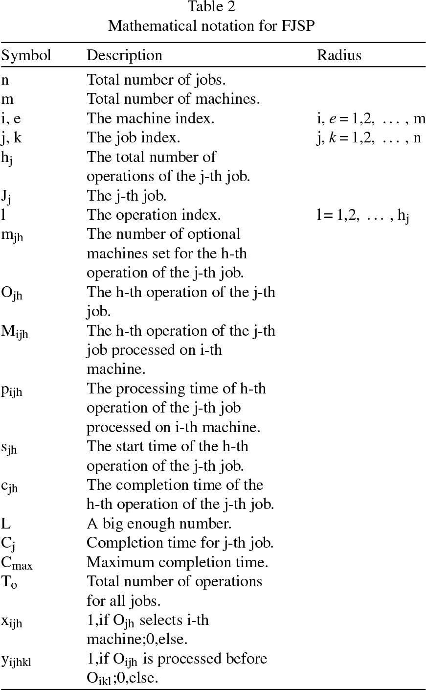
The mathematical notation for FJSP is as follows in Table 2:

{\begin{matrix} S_{jh} + x_{ijh} \cdot p_{ijh} ⩽ c_{jh} (a) \\ c_{jh} ⩽ s_{j (h + 1)} (b) \\ c_{{jh}_{j}} ⩽ C_{max} (c) \\ s_{jh} + p_{ijh} ⩽ s_{kl} + L (1 - y_{ijhkl}) (d) \\ c_{jh} ⩽ s_{j (h + 1)} + L (1 - y_{{ikl}_{j} (h + 1)}) (e) \\ \sum_{i = 1}^{m_{jh}} x_{ijh} = 1 (f) \\ \sum_{j = 1}^{n} \sum_{h = 1}^{h_{j}} y_{ijhkl} = x_{ikl} (g) \\ \sum_{k = 1}^{n} \sum_{l = 1}^{h_{k}} y_{ijhkl} = x_{ijh} (h) \\ s_{jh} ⩾ 0, c_{jh} ⩾ 0 (i) \end{matrix}

(1)

Table 2

Mathematical notation for FJSP

Symbol	Description	Radius
n	Total number of jobs.
m	Total number of machines.
i, e	The machine index.	i, e = 1,2, ... , m
j, k	The job index.	j, k = 1,2, ... , n
h_j	The total number of operations of the j-th job.
J_j	The j-th job.
l	The operation index.	l = 1,2, ... , h_j
m_jh	The number of optional machines set for the h-th operation of the j-th job.
O_jh	The h-th operation of the j-th job.
M_ijh	The h-th operation of the j-th job processed on i-th machine.
p_ijh	The processing time of h-th operation of the j-th job processed on i-th machine.
s_jh	The start time of the h-th operation of the j-th job.
c_jh	The completion time of the h-th operation of the j-th job.
L	A big enough number.
C_j	Completion time for j-th job.
C_max	Maximum completion time.
T_o	Total number of operations for all jobs.
x_ijh	1,if O_jh selects i-th machine;0,else.
y_ijhkl	1,if O_ijh is processed before O_ikl;0,else.

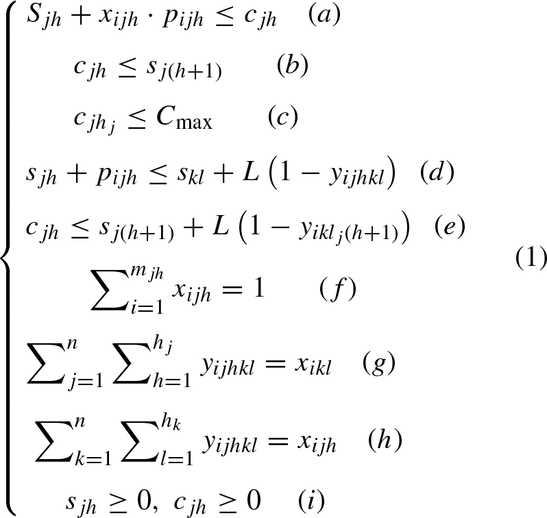
In Equation (1), (a) and (b) represent a process sequence constraint for each job; (c)represents a constraint on the completion time of the job; (d) and (e) represent that only one operation can be processed by a given operation at a given time; (f) represents that the same operation at the same time can only be processed by one machine; (g) and (h) represent that each machine has cyclic operations; (i) represents that each variable must be positive.

Evaluation: The makespan is a crucial metric that measures the time taken for all jobs to complete within a workshop. It serves as an indicator of resource utilization, production efficiency, throughput, delivery commitments, and aids in planning and coordination of operations. The makespan is determined by finding the completion time, which is the time when the last operation of each job is completed. The maximum completion time among all jobs is considered the makespan. This metric also helps in identifying bottlenecks in the production process. As is shown in Equation (2).

f = \min (max_{1 ⩽ j ⩽ n} (C_{j}))

(2)

3 Basic theory

3.1 Reinforcement learning

1. Definition

Reinforcement Learning (RL) is a significant branch of machine learning [34]. RL involves interactive learning, where agents interact with the environment through trial and error, accumulating experience and receiving feedback. This feedback is then used to learn and develop the optimal policy. The mathematical foundation of RL is built upon the Markov Decision Process, as illustrated in Fig. 1.

Fig. 1

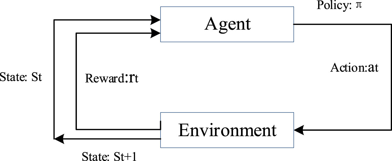
Basic reinforcement learning model.

2. Markov Decision Process

RL, also known as memoryless, exhibits the Markov property, where the feedback from the environment is solely determined by the previous state and action.The agent samples from the environment to learn an optimal action policy π^* that maximizes the cumulative reward r obtained by taking an action a at any given time step. In practical scenarios, the discounted future reward G_t is commonly employed to represent the cumulative reward in the future within time step t. G_t is shown in Equation (3).

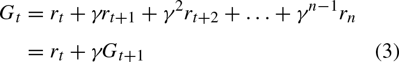
\begin{matrix} G_{t} & = r_{t} + γ r_{t + 1} + γ^{2} r_{t + 2} + \dots + γ^{n - 1} r_{n} \\ = r_{t} + γ G_{t + 1} \end{matrix}

(3)

where, γ is the discount factor.

In Equation (4), State value function v (s) represents the reward expectation obtained by performing action a under state s:

v (s) = E [r_{t + 1} + γ G_{t + 1} | s_{t} = s]

(4)

Action value function is shown in Equation (5).

q (s, a) = E [r_{t + 1} + γ G_{t + 1} | s_{t} = s, a_{t} = a]

(5)

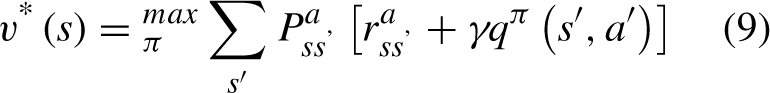
In Equation (6), The optimal value function is the value function whose value is greater than that of other functions in each state:

v^{*} (s) =_{π}^{m a x} v^{*} (s)

(6)

The Behrman equation of the value function is:

υ^{π} (s) = \sum_{a}^{} π (s, a) \sum_{s'}^{} p_{s s'}^{a} [r_{s s'}^{a} + γ υ^{π} (s')]

(7)

q^{π} (s, a) = \sum_{s'}^{} p_{s s'}^{a} [r_{s s'}^{a} + γ q^{π} (s', a')]

(8)

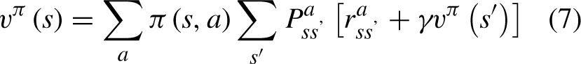
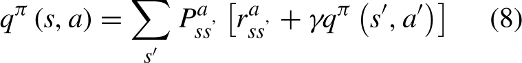
So, the most Behrmann equation can be obtained: represents the transition probability from state s to s after executing action a, represents the reward from state s to s after executing action a. v^π (s)represents the value function after executing the policy π. q^π (s, a) represents the action value function after executing the policy π.

υ^{*} (s) =_{π}^{\max} \sum_{s'}^{} p_{s s'}^{a} [r_{s s'}^{a} + γ q^{π} (s', a')]

(9)

The above process is the process of generating the optimal policy.

3.2 Policy making based on four reinforcement learning algorithms

There are several influential algorithms in RL that have been widely studied. These algorithms include the dynamic programming method, sequential difference method, Q-learning algorithm, Double-Q-learning algorithm, Sarsa algorithm, policy gradient algorithm, DQN algorithm, and PPO algorithm. In our study, we focus on using the Double-Q-learning [12], Q-learning [42], State-Action-Reward-State-Action (SARSA) [8], and State-Action-Reward-State-Action (λ) (SARSA (λ)) [19] algorithms to train the agent. In the next section, we will provide a detailed introduction to these four algorithms.

To effectively apply RL in solving practical problems, it is crucial to convert the optimization problem into a decision problem. A decision problem necessitates the existence of a policy. In this paper, four algorithm decision methods have been chosen, including the greedy policy and the ɛ-greedy policy. The greedy policy entails selecting the best solution at each step based on the current state, with the aim of eventually reaching the global best solution. On the other hand, the ɛ-greedy policy is an extension of the greedy policy. While it also selects the best solution under the current state, it also has a certain probability (ɛ) of choosing a suboptimal solution to prevent getting stuck in a local optimal solution. The Equation (10) for the ɛ-greedy policy is as follows:

\begin{matrix} π (a | s) = \\ {\begin{matrix} 1 - ɛ + \frac{ɛ}{| A (s) |}, a = \underset{a^{'}}{argmax} q (s, a^{'}) \\ \frac{ɛ}{| A (s) |}, a \neq \underset{a^{'}}{argmax} q (s, a^{'}) \end{matrix} s ɛ S, a^{'} ɛ A \end{matrix}

(10)

The policy type can be either On-Policy or Off-Policy. The policy π serves two roles in the algorithm: generating experience and improving policy. The policy that generates experience is referred to as the behavior policy, while the policy that promotes policy improvement is known as the goal policy. On-Policy refers to the scenario where the behavior policy is the same as the target policy, whereas Off-Policy refers to the scenario where the behavior policy differs from the target policy.

The SARSA algorithm is an On-Policy method with an iterative expression in Equation (11).

\begin{matrix} q (s_{t}, a_{t}) \leftarrow q (s_{t}, a_{t}) \\ + α [r_{t + 1} + γ q (s_{t + 1}, a_{t + 1}) - q (s_{t}, a_{t})] \end{matrix}

(11)

where, a_t and a_t+1 are chosen using the ɛ-greedy policy, which is determined by the estimated q values. The q values are continuously updated based on the behavior policy π, while also allowing π to approach the greedy policy based on q.

The Q-learning algorithm is a sequential difference algorithm used to solve the optimal action value. It is currently the most widely used RL algorithm. Unlike the SARSA algorithm, which requires policy improvement steps to achieve the optimal policy, Q-learning can directly estimate the optimal action value.

Q-learning algorithm is an Off-Policy method, and the iterative expression is shown in Equation (12).

\begin{matrix} q (s_{t}, a_{t}) \leftarrow q (s_{t}, a_{t}) \\ + α [r_{t + 1} + γ max_{a \in A (s_{t + 1})} q (s_{t + 1}, a) - q (s_{t}, a)] \end{matrix}

(12)

where, a_t is obtained by sampling with ɛ-greedy method based on q, but a is selected with greedy method, which is different from SARSA, namely: the behavior policy is ɛ-greedy method, and the target policy is greedy policy.

The decision-making process in the SARSA algorithm is similar to that of the Q-Learning algorithm, where the Q-table is used to determine the action to be taken based on the highest Q-value. However, the key difference between the two lies in their action update criteria. While Q-Learning selects the maximum estimated Q-value, SARSA directly selects the estimated Q-value without seeking the maximum.

When optimizing policies, the Q-Learning algorithm utilizes a q function to estimate the next state, which may lead to an overestimation problem. In contrast, the Double-Q-learning algorithm employs two q function estimation policies. Each q function updates the next state based on the value of the other q function. Both q functions must be learned from different sets of experiences, but both can be used to select actions. During the update, only one of the q functions is updated while the other is used to select the optimal action. By adopting this approach, the overestimation problem inherent in traditional Q-learning can be avoided, and the overall stability and performance of the algorithm can be significantly improved.

The iterative expression of Double-Q-learning algorithm is shown in Equation (13).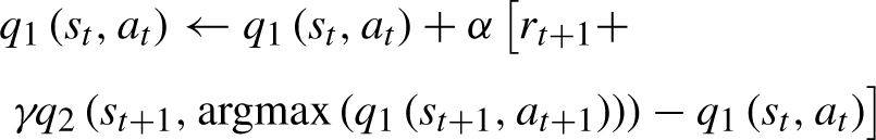

\begin{matrix} q_{1} (s_{t}, a_{t}) \leftarrow q_{1} (s_{t}, a_{t}) + α [r_{t + 1} + \\ γ q_{2} (s_{t + 1}, argmax (q_{1} (s_{t + 1}, a_{t + 1}))) - q_{1} (s_{t}, a_{t})] \end{matrix}

\begin{matrix} q_{2} (s_{t}, a_{t}) \leftarrow q_{2} (s_{t}, a_{t}) + α [r_{t + 1} + γ q_{1} (s_{t + 1}, \\ argmax (q_{2} (s_{t + 1}, a_{t + 1}))) - q_{2} (s_{t}, a_{t})] \end{matrix}

(13)

SARSA is a single-step update, referred to as SARSA(0), or n-step update, referred to as SARSA(n). To generalize these processes, we introduce the λ value to represent the number of steps, resulting in SARSA(λ). While both SARSA and Q-learning update the reward only after receiving it, SARSA(λ) updates the reward before receiving it. The λ value can range between 0 and 1.

The iterative expression of SARSA algorithm is shown in Equation (14).

\begin{matrix} q (s_{t}, a_{t}) \leftarrow q (s_{t}, a_{t}) \\ + α [r_{t + 1} + γ q (s_{t + 1}, a_{t + 1}) - q (s_{t}, a_{t})] \end{matrix}

(14)

The iterative expression of SRASR(λ)algorithm is shown in Equation (15).

\begin{matrix} q (s_{t}, a_{t}) \leftarrow q (s_{t}, a_{t}) + α δ_{t} E_{t} (s_{t}, a_{t}) \end{matrix}

E_{t} (s, a) = {\begin{matrix} γ λ E_{t - 1} (s, a) + 1 {ifs}_{t} = s, a_{t} = a \\ γ λ E_{t - 1} (s, a) otherwise \end{matrix}

(15)

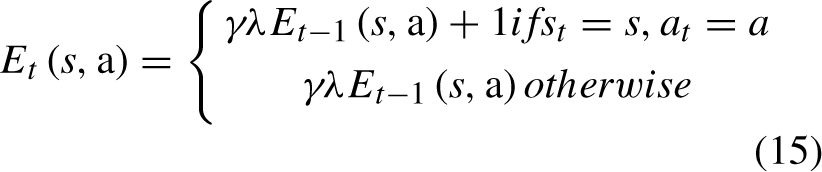
Where,δ_t epresents the Temporal Difference Error of time step t, E_t (s, a) is the eligibility trace of a certain state-action pair in time step t, λ is the parameter, 0 ⩽ λ ⩽ 1.

3.3 Variation operator of genetic algorithm

The Genetic Algorithm (GA) is an optimization search algorithm that mimics the process of natural evolution. It represents candidate solutions using genetic encoding and employs genetic operations such as selection, crossover, and variation to explore potential optimal solutions. GA is particularly useful for solving complex and challenging optimization problems.

Variation operator is one of the genetic operations in GA and is used to introduce random fluctuations into candidate solutions. This is done to increase the diversity of the search space. Commonly used variation operators include bit variation, insertion variation, and reversal variation. Bit variation is the most frequently used type of variation operation, where one or several genes of an individual are randomly assigned or flipped with a certain probability. This process helps in discovering better solutions. The role of variation operation in GA is to enhance the exploration of the solution space through random perturbations. This, in turn, helps in avoiding being trapped in local optima. Variation operation also plays a crucial role in maintaining the diversity of the population and improving the global search capability of the algorithm. To maintain the fundamental characteristics of individuals and avoid excessive disturbances, the probability of variation is usually kept low.

To represent the FJSP using the variation operator, we need to consider the encoding of operations and machines. This paper adopts an encoding method inspired by the method described in reference [52], with some improvements. It utilizes a coding method that is based on the index of the job and the index of the operation. To illustrate, let’s consider the specific example provided in Table 1.

In Table 1, the operations of Job J₁ and J₂ are listed. One possible encoding is shown in Fig. 2.

Fig. 2

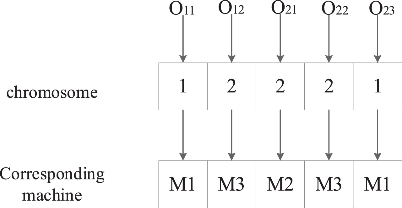
Chromosome encoding.

This encoding method organizes the operations in ascending order based on the index of the job and the index of the operation, forming a chromosome. For instance, operation O₁₁ presents two machine options: M₁ and M₃. The code ’1’ signifies selecting the first machine, which is M₁. Similarly, operation O₁₂ offers two machine choices: M₂ and M₃. The code ’2’ represents choosing the second machine, which is M₃.

Using bit variation, a specific position in the chromosome is mutated. In Fig. 2, the operation O₂₁ corresponds to the number ’2’ in the chromosome. After the bit variation, the number ’2’ changes to ’1’, indicating a change from processing on the second machine to processing on the first machine. This is illustrated in Fig. 3.

Fig. 3

Variation.

4 Transformation of scheduling problem

The key of using RL algorithm to solve FJSP is to transform the problem into a decision problem, which involves determining state space, action space, and reward function.

4.1 State space

In FJSP, the state space can easily suffer from the ‘curse of dimensionality’ due to the multiple operations and machines involved in each job. This paper proposes an approach for selecting the state space, which is outlined as follows: 1) Randomly generate a subset of the FJSP and encode them using the methods described in Section 3.3. 2) Introduce variations to the sampled instances based on a given variation rate. 3) Decode the mutated chromosomes, along with the original chromosomes, to determine the completion time of each chromosome. This completion time represents the maximum completion time in this state.

The chromosome with the minimum maximum completion time is selected to extract the state. the states obtained from the sampling on the optimal chromosome are put into memory bank D for reinforcement learning algorithm training.

Five state characteristic values, ranging from 0 to 1, are defined to represent the current states at each scheduling time point. The state can be represented as a 5-tuple in Equation (16).

s_{t} = (U_{a}, U_{s}, U_{O}, U_{Oa}, U_{Os})

(16)

An explanation of each parameter in Equation (17).

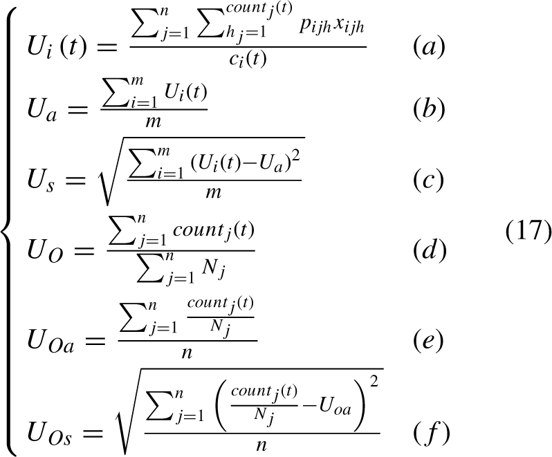
{\begin{matrix} U_{i} (t) = \frac{\sum_{j = 1}^{n} \sum_{h_{j} = 1}^{{count}_{j} (t)} p_{ijh} x_{ijh}}{c_{i} (t)} & (a) \\ U_{a} = \frac{\sum_{i = 1}^{m} U_{i} (t)}{m} & (b) \\ U_{s} = \sqrt{\frac{\sum_{i = 1}^{m} {(U_{i} (t) - U_{a})}^{2}}{m}} & (c) \\ U_{O} = \frac{\sum_{j = 1}^{n} {count}_{j} (t)}{\sum_{j = 1}^{n} N_{j}} & (d) \\ U_{Oa} = \frac{\sum_{j = 1}^{n} \frac{{count}_{j} (t)}{N_{j}}}{n} & (e) \\ U_{Os} = \sqrt{\frac{\sum_{j = 1}^{n} {(\frac{{count}_{j} (t)}{N_{j}} - U_{oa})}^{2}}{n}} & (f) \end{matrix}

(17)

Where,

C_i (t) represents the completion time of the last operation on i-th machine at time t.

count_j (t) represents the number of completed operations for j-th job at time t.

N_j represents the number of operations in j-th job.

(a) represents the utilization rate of i-th machine at scheduling time t.

(b) represents the average utilization of machines.

(d) represents the total completion rate of the operation.

(e) represents the average completion rate of job.

(f) represents the standard deviation of job completion rate.

This method extracts the state space from an optimal solution and defines 5 variables as reinforcement learning to solve the FJSP state. This approach makes it easier to obtain the final optimal solution.

4.2 Action space

When studying action space scheduling rules, many researchers have adopted traditional scheduling rules and achieved excellent results. For example, Liu C et al. [21] proposed a parallel training method that utilized the scheduling rule of selecting the job with the shortest processing time. Lin C-C [24] et al. introduced an intelligent manufacturing plant framework based on edge computing and further investigated the JSP under this framework, employing the selection of the job with the longest processing time as the scheduling rule. Shiue, Y. R. et al. [35] proposed an RTS based on RL that utilized the MDRs mechanism and selected the job with the shortest remaining processing time as the scheduling rule. Han, B.A et al. [14] proposed a deep reinforcement learning framework based on disjunctive graph scheduling, where the scheduling rule was to select the job with the longest processing time. Wang Y C et al. [38] conducted a factorial experiment design to study the application of Q-learning to the setting of the single-machine scheduling rule selection problem, using first-come-first-served as the scheduling rule.

Due to the complexity of FJSP, there are two decisions to choose the process, traditional scheduling rules are not suitable for solving this problem. To address this, this paper proposes a 4-tuple representation for the action space. The 4-tuple includes the job, the operation of the job, the selected machining machine for the operation, and the processing time of the operation on the selected machine. This representation can be expressed as Equation (18).

a (s) = (J_{j}, O_{jh}, M_{ijh}, p_{ijh})

(18)

For example, the expression of action space in Table 1 is shown in Fig. 4.

Fig. 4

An action.

4.3 Reward

When studying FJSP, the agent receives a reward from the environment, which serves as a continuous motivation for the agent’s learning process. As a result, the reward function should aim to maximize the immediate impact of each action taken by the agent, while also ensuring that the cumulative reward aligns with the optimization of the objective function. Currently, the most commonly used method for the reward function in solving FJSP is the single-step transfer time. This particular reward function incentivizes the algorithm to efficiently complete all the jobs as quickly as possible, and it is mathematically represented by Equation (19).

r = - (C_{\max}^{n + 1} - C_{\max}^{n})

(19)

Where, $C_{\max}^{n}$ is the maximum completion time of round n.

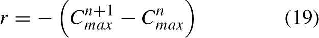
4.4 Technical route

The Technical route is shown in Fig. 5.

Fig. 5

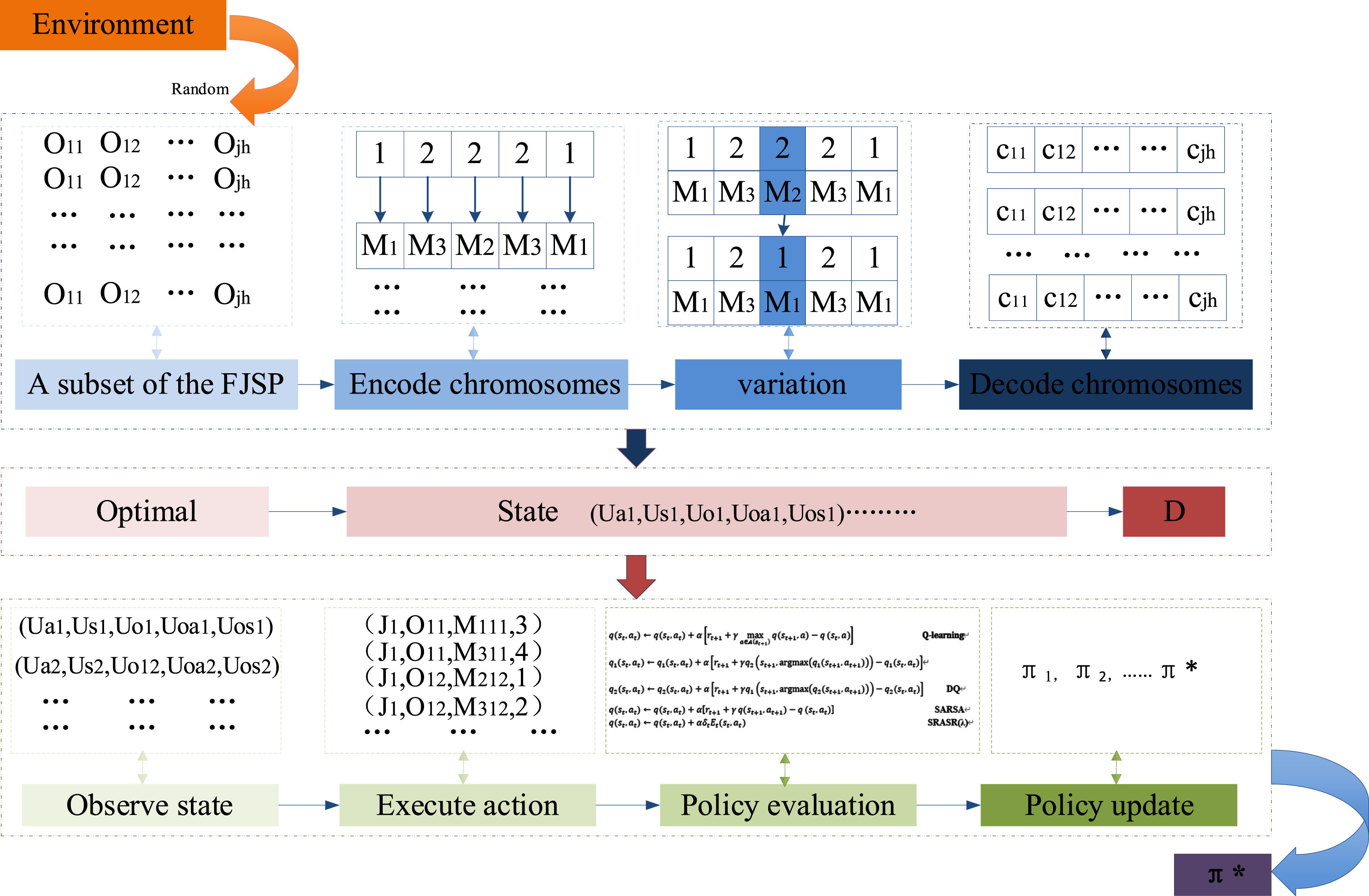
Technical route.

4.5 Training Algorithm

5 Simulation experiment results

This paper first selected the widely used Mk series of FJSP classic examples to verify the effectiveness of the four algorithms. The Mk data Brandimarte [31] is randomly generated using a uniform distribution within a given range. The data includes the number of jobs, the number of machines, the minimum and maximum number of processes per job, the maximum number of machines that can be selected before the process, and the maximum and minimum processing time of each process. Both the training and testing sets in this study used ten instances of the Mk01 to Mk10, which constitute a publicly available dataset. The problem size ranges from 10×5 to 30×10.

The algorithm program in this paper was implemented in Pycharm using the Python 3.8 programming language. The experimental platform consisted of an Intel Core i5-10600KF CPU and NVIDIA GeForce GTX 1050 Ti GPU, running on a 64-bit Windows 10 system.

After multiple parameter adjustments, the following training parameters were set: Iteration number L: 100000; Random factor ɛ: 0.95; Discount factor γ: 0.95; Learning rate α: 0.03; Qualified trace attenuation factor λ: 0.95; Sampling size: 200; Variation rate: 0.55, D size: 100.

After 10 control parameter experiments, it was found that the convergence of this method is slow, with an average convergence of ten tests at around 80,000 iterations. Therefore, the number of iterations L is chosen. The choice of ɛ for preserving some of the exploratory nature is based on the need to retain the return from the previous state. The value of α changes with the number of iterations. overall, this parameter has shown a positive impact.

5.1 Comparison between the proposed algorithm and other reinforcement learning algorithms

This study utilized a random sampling technique to select FJSP instances and encode them. To introduce diversity to the instances, the genetic algorithm variation operator was employed. After decoding, the chromosome with the smallest maximum completion time was chosen for state extraction. The state space was constructed using five features at time t, and the FJSP model was solved using four RL algorithms mentioned earlier. The performance of different examples in minimizing the maximum completion time optimization goal varied. Comparison algorithms, GA-Q and GA-SARSA, adopted from the literature [4], were used in this study. The makespan results are presented in Table 3.

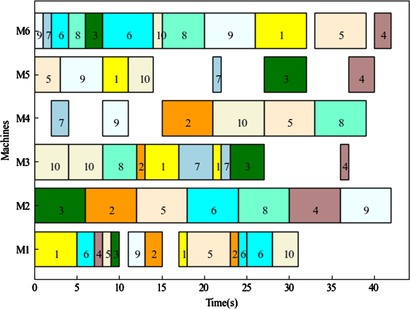
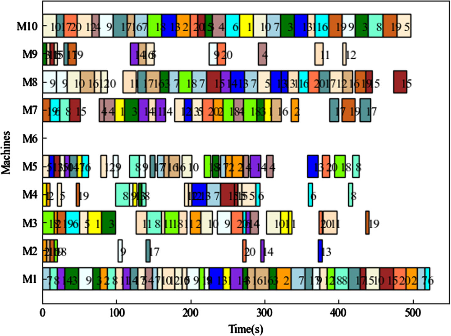
BKS represents the theoretical optimal solution. Based on the findings presented in Table 3, the proposed model showcases significant optimization effects for examples mk01, mk03, mk04, mk05, mk08, mk09, and mk10. However, it shows slightly lower performance on other examples. Notably, the Q-learning achieves the theoretical optimal solution for mk03 and mk08. The Gantt charts for mk01, mk08, and mk10 scheduling are illustrated in Fig. 6, Fig. 7, and Fig. 8, respectively.

Table 3
Compared with some reinforcement learning algorithms

Algorithm BKS GA-Q GA-SARSA DQ Q SARSA SARSA(λ)

mk01(106) 36 44.1 43.2 42 42* 44 48

mk02(106) 24 32.3 31.8 38 41 39 44

mk03(158) 204 214.9 211.7 207 204 216 211

mk04(158) 48 78.1 73.1 74 73 75 85

mk05(154) 168 187.4 185.8 182 185 195 194

mk06(1010) 33 82.3 80.3 93 94 95 99

mk07(205) 133 159.9 156.7* 206 206 211 211

mk08(2010) 523 529.6 539.4 524 523 540 557

mk09(2010) 299 354.6 331.8 339 329 349 349

mk10(2015) 165 287.2 281.2 269 261 294 298

Algorithm	BKS	GA-Q	GA-SARSA	DQ	Q	SARSA	SARSA(λ)
mk01(10*6)	36	44.1	43.2	42*	42*	44	48
mk02(10*6)	24	32.3	31.8*	38	41	39	44
mk03(15*8)	204	214.9	211.7	207	204*	216	211
mk04(15*8)	48	78.1	73.1	74	73*	75	85
mk05(15*4)	168	187.4	185.8	182*	185	195	194
mk06(10*10)	33	82.3	80.3	93	94	95	99
mk07(20*5)	133	159.9	156.7*	206	206	211	211
mk08(20*10)	523	529.6	539.4	524	523*	540	557
mk09(20*10)	299	354.6	331.8	339	329*	349	349
mk10(20*15)	165	287.2	281.2	269	261*	294	298

Fig. 6

A Gantt chart of mk01.

Fig. 7

A Gantt chart of mk08.

Fig. 8

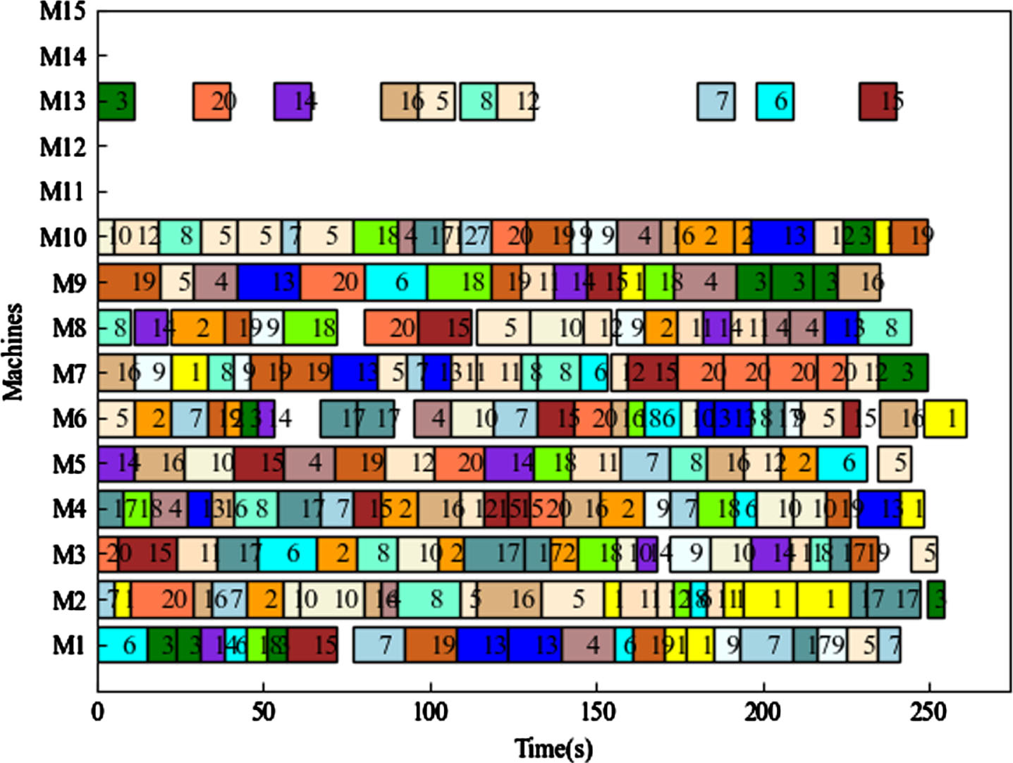
A Gantt chart of mk10.

The figure above demonstrates that the arrangement of Mk01, using the method described in this article, outperforms other algorithms. This indicates that the method is effective for small-scale production scheduling. However, it should be noted that Mk08 does not have any processes arranged on M6, and Mk10 does not have any processes arranged on M11, M12, M14, and M15. This is because these machines either cannot process all the operations or take too long to process them. The Gantt charts visually represent the distribution of tasks on a timeline for completing a job, allowing you to observe the start time and completion time of each job. By implementing the algorithm proposed in this article, a better task allocation strategy can be achieved, resulting in an improved maximum completion time.

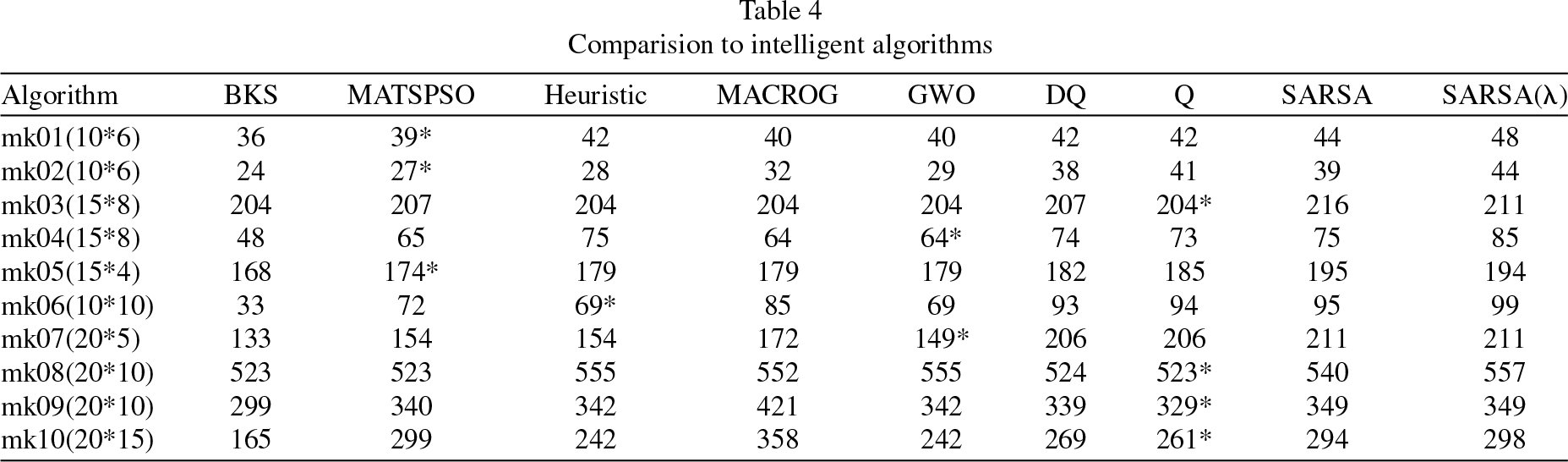
This article compares an established model with several intelligent algorithms, including a hybrid algorithm of tabu search and particle swarm optimization (MATSPSO) [15], a heuristic algorithm based on construction scheduling rules (Heuristic) [53], a multi-agent model algorithm based on chemical reaction optimization and greedy meta-heuristics (MACROG) [29], and the Gray Wolf Optimization Algorithm (GWO) [16]. The experimental results are presented in Table 4. From Table 4, it can be observed that the framework proposed in this article, when using the Q-learning algorithm, outperforms all other algorithms on mk03, mk08, mk09, and mk10, and achieves two optimal solutions. Moreover, the results of the Double-Q-learning algorithm also outperform some intelligent algorithms, indicating that this method is suitable for solving larger models.

Table 4

Comparision to intelligent algorithms

Algorithm	BKS	MATSPSO	Heuristic	MACROG	GWO	DQ	Q	SARSA	SARSA(λ)
mk01(10*6)	36	39*	42	40	40	42	42	44	48
mk02(10*6)	24	27*	28	32	29	38	41	39	44
mk03(15*8)	204	207	204	204	204	207	204*	216	211
mk04(15*8)	48	65	75	64	64*	74	73	75	85
mk05(15*4)	168	174*	179	179	179	182	185	195	194
mk06(10*10)	33	72	69*	85	69	93	94	95	99
mk07(20*5)	133	154	154	172	149*	206	206	211	211
mk08(20*10)	523	523	555	552	555	524	523*	540	557
mk09(20*10)	299	340	342	421	342	339	329*	349	349
mk10(20*15)	165	299	242	358	242	269	261*	294	298

5.2 Dispersion of solutions of four reinforcement learning algorithms

In this paper, four reinforcement learning algorithms were used to establish a solving model. The model was trained using the mk01 dataset, and after obtaining the optimal model, it was applied to solve the mk01 to mk10 datasets. We will now analyze the discreteness of the solutions. Figure 9 presents the box plots of the four algorithms during training.

Fig. 9

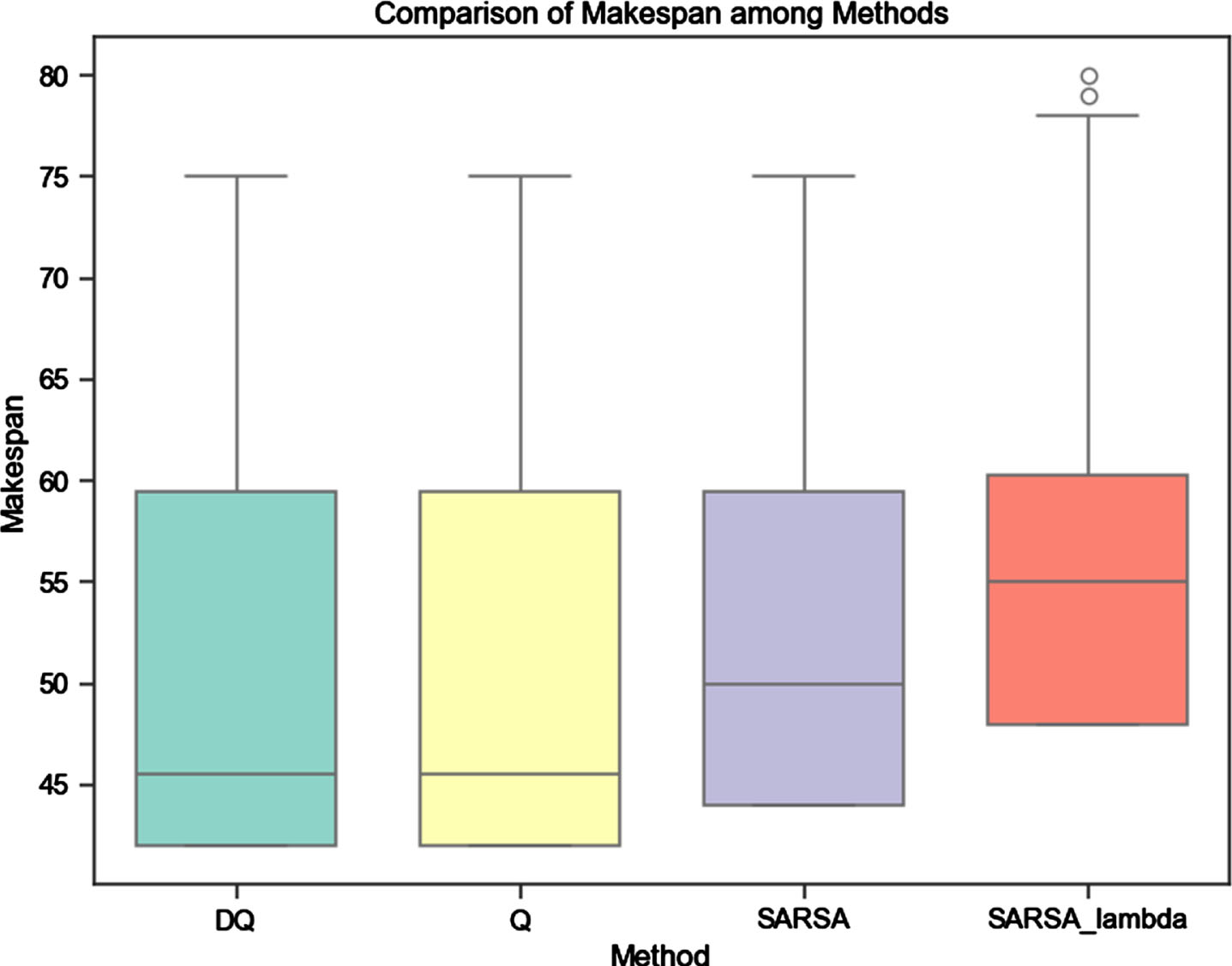
Box plots of the four algorithms during training.

From the height and width of the box plot-s, it can be observed that during the training o-f the FJSP model using variation operator and the four reinforcement learning algorithms, Double Q-learning converges the fastest, followed by Q-learning and SARSA, while SARSA(λ) has the slowest convergence speed. The solutions of Double Q-learning and Q-learning models are mostly located in smaller positions, while the solutions of SARSA(λ) algorithm are larger. It can be seen that, under the proposed state space, action space, and reward function in this study, the optimal solutions of Double Q-learning and Q-learning are more concentrated.

6 Conclusion and discussion

This paper investigates the problem of establishing a FJSP model using a variation operator based on genetic algorithms and reinforcement learning algorithms. Considering the large number of states involved in this problem, the curse of dimensionality is likely to occur. To address this issue, this study adopts random sampling to extract partial states and utilizes the variation operator to increase the diversity of these chromosomes. After decoding, the optimal solutions are selected to participate in the state extraction process of the Markov decision process. In order to ensure sufficient state extraction, this study designs 5-tuple as states. The action space is designed as a 4-tuple, and the reward function is devised in a way that the direction of cumulative reward increase aligns with the optimization direction of the objective function. This approach offers a fresh perspective for reinforcement learning in solving FJSP.

The experimental results demonstrate that: (1)

Both Double-Q learning and Q-learning algorithms demonstrate rapid adaptation to various FJSPs and constraints.

(2)

The optimization of the Q-value function enhances the robustness and scalability of these algorithms.

(3)

RL algorithms generate solutions that comply with constraints without explicitly representing them.

(4)

Compared to traditional algorithms, RL algorithms exhibit greater flexibility in handling constraints.

(5)

RL algorithms leverage techniques such as simulation and emulation for offline training, which effectively reduces cost and risk.

The advantages of RL algorithms, their flexibility in handling constraints, and their ability to generate constraint-compliant solutions make them valuable for solving FJSP. However, the research on RL for FJSP is limited compared to JSP. This study introduces a unique approach combining variation operator with RL for FJSP, providing new insights. Challenges like training instability and slow convergence speed need further investigation in future research.

Footnotes

Acknowledgments

This work is supported by the Key Project 2020 of the Ministry of Science and Technology of China-Research on Real-time Operation Optimization Technology of Production Line Driven by Data Intelligence. (No.2020YFB1712202).

References

Azzouz

Ennigrou

Said

L.B.

, A hybrid algorithm for flexible job-shop scheduling problem with setup times, International Journal of Production Management & Engineering5(1) (2017), 23–30.

Türkylmaz

Bulkan

, A hybrid algorithm for total tardiness minimisation in flexible job shop: Genetic algorithm with parallel VNS execution, International Journal of Production Research53(6) (2015), 1832–1848.

Buddala

Sankar

, Mahapatra, An integrated approach for scheduling flexible job-shop using teaching–learning-based optimization method, Journal of Industrial Engineering International15(1) (2019), 181–192.

Chen

, et al., A self-learning genetic algorithm based on reinforcement learning for flexible job-shop scheduling problem,&, Industrial Engineering149 (2020), 106778.

Chang , et al., Deep reinforcement learning for dynamic flexible job shop scheduling with random job arrival, Processes10(4) (2022), 760.

, Event scheduling algorithm of phased array radar based on branch and bound method, Acta Electronica Sinica6 (2019), 1309–1314.

, et al., A reinforcement learning approach for flexible job shop scheduling problem with crane transportation and setup times, IEEE Transactions on Neural Networks and Learning Systems (2022), 1–15.

Dongbin

, et al., Deep reinforcement learning with experience replay based on SARSA, 2016 IEEE symposium series on computational intelligence (SSCI). IEEE, 2016.

Dauzère-Pérès

, et al., The flexible job shop scheduling problem: A review, European Journal of Operational Research (2023).

10.

Gaham

Bouzouia

Achour

, An effective operations permutation-based discrete harmony search approach for the flexible job shop scheduling problem with makespan criterion, Applied Intelligence48 (2018), 1423–1441.

11.

Chang

H.C.

Liu

T.K.

, Optimisation of distributed manufacturing flexible job shop scheduling by using hybrid genetic algorithms, Journal of Intelligent Manufacturing28 (2017), 1973–1986.

12.

Hasselt

, Van, A. Guez and D. Silver, Deep reinforcement learning with double q-learning, Proceedings of the AAAI conference on artificial intelligence30(1). 2016.

13.

Han

Yang

, A deep reinforcement learning based solution for flexible job shop scheduling problem, International Journal of Simulation Modelling20(2) (2021), 375–386.

14.

Han

B.-A.

Yang

J.-J.

, Research on adaptive job shop scheduling problems based on dueling double DQN, IEEE Access8 (2020), 186474–186495.

15.

Henchiri

Ennigrou

, Particle swarm optimization combined with tabu search in a multi-agent model for flexible job shop problem, Advances in Swarm Intelligence: 4th International Conference, ICSI 2013, Harbin, China, June 12–15, 2013, Proceedings, Part II 4. Springer Berlin Heidelberg, 2013.

16.

Jiang

Zhang

, Application of grey wolf optimization for solving combinatorial problems: Job shop and flexible job shop scheduling cases, IEEE Access6 (2018), 26231–26240.

17.

Johnson

S.M.

, Optimal two-and three-stage production schedules with setup times included, Naval research logistics quarterly1(1) (1954), 61–68.

18.

Jalilvand-Nejad

Fattahi

, A mathematical model and genetic algorithm to cyclic flexible job shop scheduling problem, Journal of Intelligent Manufacturing26 (2015), 1085–1098.

19.

Jiang

, et al., An Improved Sarsa(λ) Reinforcement Learning Algorithm for Wireless Communication Systems, IEEE Access7 (2019), 115418–115427.

20.

, et al., An effective MCTS-based algorithm for minimizing makespan in dynamic flexible job shop scheduling problem, Computers & Industrial Engineering155(1) (2021), 107211.

21.

Liu

Chang

Tseng

, Actor-Critic Deep Reinforcement Learning for Solving Job Shop Scheduling Problems, IEEE Access (2020), 71752–71762.

22.

Long , et al., A self-learning artificial bee colony algorithm based on reinforcement learning for a flexible job-shop scheduling problem, Concurrency and Computation: Practice and Experience34(4) (2022), e6658.

23.

, et al., Reinforcement learning based VNF scheduling with end-to-end delay guarantee, 2019 IEEE/CIC International Conference on Communications in China (ICCC). IEEE, 2019.

24.

Lin

C-C.

, et al., Smart manufacturing scheduling with edge computing using multiclass deep Q network, IEEE Transactions on Industrial Informatics15(7) (2019), 4276–4284.

25.

Lim

K.C.W.

Wong

L.-P.

Chin

J.F.

, Simulated-annealing-based hyper-heuristic for flexible job-shop scheduling, Engineering Optimization55(10) (2023), 1635–1651.

26.

Luo

, Dynamic scheduling for flexible job shop with new job insertions by deep reinforcement learning, Applied Soft Computing91 (2020), 106208.

27.

, et al., A memetic algorithm for solving flexible job-shop scheduling problems, 2014 IEEE Congress on Evolutionary Computation (CEC). IEEE, 2014.

28.

Meng

Pan

Q.-K.

Sang

H.-Y.

, A hybrid artificial bee colony algorithm for a flexible job shop scheduling problem with overlapping in operations, International Journal of Production Research56(16) (2018), 5278–5292.

29.

Marzouki

Belkahla Driss

, Ghédira

,Multi agent model based on chemical reaction optimization with greedy algorithm for flexible job shop scheduling problem, Procedia Computer Science112 (2017), 81–90.

30.

Phu-ang

Thammano

, Memetic algorithm based on marriage in honey bees optimization for flexible job shop scheduling problem, Memetic Computing9 (2017), 295–309.

31.

Brandimarte

, Routing and scheduling in a flexible job shop by tabu search, Annals of Operations Research41(3) (1993), 157–183.

32.

Suryaputra

Setiawan

, Reinforcement learning combined with radial basis function neural network to solve job-shop scheduling problem, 2011 IEEE International Summer Conference of Asia Pacific Business Innovation and Technology Management. IEEE, 2011.

33.

Ren

Sun

, Immune genetic algorithm for multi-objective flexible job-shop scheduling problem, 2016 Chinese control and decision conference (CCDC). IEEE, 2016.

34.

Richard

, Reinforcement learning: An introduction, MIT press, 2018.

35.

Shiue

Y.-R.

Lee

K.-C.

C.-T.

, Real-time scheduling for a smart factory using a reinforcement learning approach, Computers & Industrial Engineering125 (2018), 604–614.

36.

Wang

, et al., Flexible job shop scheduling problem using an improved ant colony optimization, Scientific Programming2017 (2017).

37.

Wang

Zhu

, A hybrid genetic algorithm for flexible job shop scheduling problem with sequence-dependent setup times and job lag times, IEEE Access9 (2021), 104864–104873.

38.

Wang

Y.C.

Usher

J.M.

, Learning policies for single machine job dispatching, Robotics & Computer Integrated Manufacturing20(6) (2004), 553–56213.

39.

Minghua

, Simulation and Optimization of Lean Production Line Layout Based on Flexsim, Tianjin University, 2011.

40.

Zhang

, Thomas Dietterich

, A reinforcement learning approach to job-shop scheduling, IJCAI95, 1995.

41.

Wang

Luo

Cai , A variable interval rescheduling strategy for dynamic flexible job shop scheduling problem by improved genetic algorithm, Journal of Advanced Transportation2017 (2017).

42.

Christopher Watkins

JCH.

Dayan

,Q-learning, Machine Learning8(3-4) (1992), 279–292.

43.

Xie

Gao

Peng

, et al., Review on flexible job shop scheduling, IET Collaborative Intelligent Manufacturing1(3) (2019), 67–77.

44.

Zhang

Gao

, A hybrid genetic algorithm and tabu search for a multi-objective dynamic job shop scheduling problem, International Journal of Production Research51(12) (2013), 3516–3531.

45.

Zhang

, et al., A novel job-shop scheduling strategy based on particle swarm optimization and neural network, International Journal of Simulation Modelling18(4) (2019), 699–707.

46.

Zhang

, et al., Multidirection update-based multiobjective particle swarm optimization for mixed no-idle flow-shop scheduling problem, Complex System Modeling and Simulation1(3) (2021), 176–197.

47.

Zhang

, An improved genetic algorithm for the re-entrant and flexible job-shop scheduling problem, 2016 Chinese Control and Decision Conference (CCDC). IEEE, 2016.

48.

Zeng

Wang

, A chaotic simulated annealing and particle swarm improved artificial immune algorithm for flexible job shop scheduling problem, EURASIP Journal on Wireless Communications and Networking2018 (2018), 1–10.

49.

Zhu

, et al., Low carbon flexible job shop scheduling problem considering worker learning using a memetic algorithm, Optimization and Engineering21 (2020), 1691–1716.

50.

Zeng

Bai

, A Deep Reinforcement Learning Approach to Flexible Job Shop Scheduling, 2022 IEEE International Conference on Systems, Man, and Cybernetics (SMC). IEEE, 2022.

51.

Zhang

J.-D.

, et al., DeepMAG: Deep reinforcement learning with multi-agent graphs for flexible job shop scheduling, Knowledge-Based Systems259 (2023), 110083.

52.

Zhang

Gao

Shi

, An effective genetic algorithm for the flexible job-shop scheduling problem, Expert Systems with Applications38(4) (2011), 3563–3573.

53.

Ziaee

, A heuristic algorithm for solving flexible job shop scheduling problem, The International Journal of Advanced Manufacturing Technology71 (2014), 519–528.

Job	Operation	Optional machine
		M₁	M₂	M₃
J₁	O₁₁	3	–	4
	O₁₂	–	1	2
J₂	O₂₁	9	8	–
	O₂₂	–	4	5
	O₂₃	10	–	10