Method for wind power forecasting based on support vector machines optimized and weighted composite gray relational analysis

Abstract

This study proposes a weighted composite approach for grey relational analysis (GRA) that utilizes a numerical weather prediction (NWP) and support vector machine (SVM). The approach is optimized using an improved grey wolf optimization (IGWO) algorithm. Initially, the dimension of NWP data is decreased by t-distributed stochastic neighbor embedding (t-SNE), then the weight of sample coefficients is calculated by entropy-weight method (EWM), and the weighted grey relational of data points is calculated for different weather numerical time series data. At the same time, a new weighted composite grey relational degree is formed by combining the weighted cosine similarity of NWP values of the historical day and to be measured day. The SVM’s regression power prediction model is constructed by the time series data. To improve the accuracy of the system’s predictions, the grey relational time series data is chosen as the input variable for the SVM, and the influence parameters of the ideal SVM are discovered using the IGWO technique. According to the simulated prediction and analysis based on NWP, it can be observed that the proposed method in this study significantly improves the prediction accuracy of the data. Specifically, evaluation metrics such as root mean squared error (RMSE), regression correlation coefficient (r²), mean absolute error (MAE) and mean absolute percent error (MAPE) all show corresponding enhancements, while the computational burden remains relatively low.

Keywords

t-SNE power forecasting IGWO NWP

1 Introduction

The intrinsic stochastic nature and intermittency of solar and wind energy sources present formidable challenges and technical limitations in achieving accurate power generation forecasts. The absence of a robust theoretical underpinning for solar/wind power forecasting indirectly contributes to phenomena such as curtailment of surplus energy. Accurate forecasting of solar/wind power not only augments the operational efficiency of solar/wind farms but also plays a pivotal role in supporting the power dispatch department in guaranteeing the secure, stable, and economically viable operation of the grid subsequent to the substantial integration of solar/wind energy resources. The production of power is resilient may thus be improved in the power system by upgrading the wind power forecast technology [1]. The numerical weather prediction (NWP) is connected to the power output when taking into account the time series-related data it contains. For this reason, different classifications of wind power climate data have a direct impact on improving prediction accuracy [2].

In recent years, the depth and breadth of machine learning techniques have been extensively explored and have seen significant advancements. These techniques are increasingly being applied across a wide range of industries, including but not limited to healthcare, finance, automotive, and especially in renewable energy sectors. It has become instrumental in forecasting power generation from renewable sources, such as solar and wind, where traditional methods fall short due to the inherent unpredictability of these resources. Machine learning algorithms are capable of processing vast amounts of data from various sources, including weather patterns and historical energy production data, to make more accurate predictions [3 –5]. In reference [6] uses the classification and classification of strong convective weather to prove the correlation between wind speed fluctuation and meteorological nature. In reference [7], NWP and meteorological observation data of meteorological stations are used for wind power prediction. Then use three machine learning algorithms-support vector regression, artificial neural network (ANN), and Gaussian processes-to combines and forecast the data. Then, the results of the three algorithms are mixed with the mean of the Bayesian model to generate a set prediction. In reference [8], clustering analysis is used to effectively extract the wind characteristics of the same type of time period, conduct modeling analysis, and improve forecast accuracy through a systematic approach. In reference [9], to improve the predicted accuracy of the combined model that was produced as a consequence, the redundancy is eliminated by the use of grey relational analysis (GRA), and the relationship between the anticipated and actual power series of each individual model is examined. The above-mentioned wind power prediction methods based on NWP all adopt a feature extraction approach that “degrades” to adapt to clustering methods, failing to capture the dynamic changes in weather over continuous time periods. There may be scenarios where the dynamics of change are different but the feature quantities are similar, which weakens the effectiveness of weather categorization for wind power, thereby impacting the parameter selection of the wind power prediction model.

Wind power prediction methods mainly cover the time series method [10], ANN [11], support vector machines (SVM) [12], etc. The time series approach is one of them and is straightforward and simple to use, although it is less accurate than other methods. ANN technology offers the capacity for adaptive learning, and the research time is longer in the application field, but the training samples are higher. Thus, the outcome is not the world’s best answer. While SVM are popular due to their practical utility, they face challenges in the realm of parameter optimization. Consequently, there is a necessity for further refinement of its parameters to enhance the operational performance of SVM, ensuring a more effective and efficient application in various fields.

Among the parameter optimization methods based on SVM, the widely used algorithms include Particle Swarm Optimization (PSO) [13], Grid Search (GS) [14], Artificial Bees Colony (ABC) [15], etc. A quick convergence rate is achieved through PSO, but the solution is locally optimal. Among them, the particle swarm algorithm and the artificial group peak algorithm converge faster, but they are also locally optimal. The nature of GS work is system-indiscriminately search, cross-validation using parameters, comprehensive and intuitive, and global optimal solution can be obtained. However, a more comprehensive search interval results in longer search times and a large number of invalid operations. In 2014, the grey wolf optimization (GWO) algorithm [16, 17], a revolutionary swarm intelligence optimization technique is proposed, which is simple to realize and has fewer adjusting parameters. It is proved to be better than the PSO algorithm [18]. Based on parameter tuning and convergence speed and has a self-adaptive adjustment of convergence factor and pyramid hierarchy, which may balance the benefits of global retrieval and local optimization. As a result, it performs better in terms of accuracy and convergence rate.

To address the issue of parameter optimization in SVM, and considering the connection between NWP and the wind power prediction model, a wind power prediction method based on weighted composite index grey relational analysis and SVM has been proposed. At first, we use the non-linear dimension reduction method of t-distributed stochastic neighbour embedding (t-SNE) to lower the dimensionality of the Meteorological Indices in NWP and filter out the noise. Second, we use the entropy weight method (EWM) to calculate the relative importance of the various meteorological variables and wind power for our reduced-dimensional sample set. To get a better selection of relational degree, a new composite index is merged using the weighted cosine similarity [19] and the grey weighted relational degree. The improved GWO is used to optimise the parameters in order to establish the ideal settings, which in turn improves forecast precision and operational efficiency. Unlike conventional time series, ANN, or traditional SVM methods that either lack accuracy or face parameter optimization challenges, the proposed method effectively harnesses the complex interplay of meteorological data and wind power output. Through sophisticated machine learning algorithms and innovative optimization techniques, this study establishes a new benchmark for accuracy and efficiency in wind power forecasting, making a contribution to the sustainable and efficient utilization of renewable energy resources.

2 Weighted composite indicator gray relational analysis

2.1 Dimensionality reduction using t-SNE

NWP provides a large number of meteorological indicators, usually based on experience to screen out the relevant indicators, but there are always indicators affecting wind power output in the data types, so the indicators screened by experience can not be directly related to wind power output. Related and redundant meteorological indicators will increase the calculation amount of the prediction system and also reduce the prediction accuracy. The approach of extracting primary components may be used to guarantee that the NWP data model is more accurate. A multivariate data analysis technique called principle component analysis (PCA) [20] may convert a collection of linked variables into new, uncorrelated ones called principal components, which include the majority of the original data set’s total variability. In reference [21], principal component analysis is carried out, and a binary model is extracted from five original variables to simulate the power consumption of office buildings. It has been extensively reported how crucial it is to reduce the dimensionality of the input data and choose the right model variables. In this paper, the t-SNE [22, 23] dimension reduction method is used.

Distributed Stochastic Neighbor Embedding (SNE) is the foundation of the enhanced method known as t-SNE. The main function of this is to measure the similarity between data points in both low-dimensional and high-dimensional spaces, which is appropriate for reducing high-dimensional data to low-dimensional data for presentation. The Gauss joint distribution P is used to measure similarity in high-dimensional space instead of the Euclidean distance between data points, the distance distribution in low-dimensional space is expressed by the joint distribution Q which obeys the t distribution with degree of freedom 1, the cost function is written by Kullback-Leibler divergence and the optimization result is obtained by gradient descent method so that the distance distribution in high-dimensional space and low-dimensional space is as close as possible. If the n-dimensional data set is Z = (z₁, z₂, . . . , z_n) ^T, the conditional distribution probability between z_i and z_j is p_j|i, the joint distribution probability is p_ij, and the joint distribution probability between v_i and v_j is q_ij, then conditional probability p_j|i can be obtained: $p_{j | i} = \frac{exp (- {∥ z_{i} - z_{j} ∥}^{2} / (2 σ_{i}^{2}))}{\sum_{k \neq i} exp (- {∥ z_{i} - z_{k} ∥}^{2} / (2 σ_{i}^{2}))}$ (1) $p_{ij} = \frac{p_{j | i} + p_{i | j}}{2 n}$ (2) $q_{ij} = \frac{(1 + {∥ v_{i} - v_{j} ∥}^{2})^{- 1}}{\sum_{k \neq l} (- {∥ v_{k} - v_{l} ∥}^{2})^{- 1}}$ (3)

Where σ_i is the Gaussian distribution’s standard deviation with the data point in its center. To express the best I through binary search, T-SNE makes use of the perplexity σ_i. The confusion is: $perp (P_{i}) = 2^{H (P_{i})}$ (4) $H (P_{i}) = - \sum {jp}_{j | i} {log}_{2} p_{j | i}$ (5)

Where H(P_i) is the entropy of P_i. After dimension reduction, the distribution P and Q should be close to each other as much as possible. If the local features remain intact after dimension reduction, then p_ij = q_ij. The objective function of Kullback Leibler divergence is: $T = KL (P ∥ Q) = \sum_{i} \sum_{j} p_{ij} log \frac{p_{ij}}{q_{ij}}$ (6)

To minimize the objective function, the gradient descent approach is used. The iteration update and solution formula are as follows: $\frac{δ T}{δ v_{i}} = 4 \sum_{j} (p_{ij} - q_{ij}) (v_{i} - v_{j}) (1 + {∥ v_{i} - v_{j} ∥}^{2})^{- 1}$ (7) $φ^{(t)} = φ^{(t - 1)} + η \frac{δ T}{δ φ} + d (t) (φ^{(t - 1)} - φ^{(t - 2)})$ (8)

Where φ^(t) is The t iteration’s solution, and η is the pace of dimension learning. d(t) is the t iteration’s momentum.

2.2 Gray relational analysis

Grey system theory has been extensively used as an interdisciplinary technique. An essential component of grey system theory is GRA [24, 25], which quantifies how closely related distinct factors are based on whether they have the same or divergent development trends. GRA has several uses, including in the fields of information technology [26], finance [27], and industry [28]. The weather sample set composed of the dimensionally reduced multivariate index data has X = ( X₁ , X₂ , ... , X_N )^T, and the eigenvector of the i-th sample X_i can be expressed as: $X_{i} = [x_{i} (1), x_{i} (2), . . ., x_{i} (m)]$ (9)

The characteristic vectors of the test samples are: $X_{0} = [x_{0} (1), x_{0} (2), . . ., x_{0} (m)]$ (10)

The grey relational degree between two series samples can be obtained [29]: $ξ_{i} (j) = \frac{Δ_{min} + ρ Δ_{max}}{Δ_{i} (j) + ρ Δ_{max}}$ (11)

Where, ξ_i (j) is the characteristic correlation coefficient of x₀ (j) and x_i (j); $Δ_{min} = min_{i} min_{j} | x_{0} (j) - x_{i} (j) |$ ; $Δ_{max} = max_{i} max_{j} | x_{0} (j) - x_{i} (j) |$ , Δ_i (j) = |x₀ (j) - x_i (j) |, and the resolution coefficient ρ= 0.5. $F^{'} = \frac{1}{m} \sum_{j = 1}^{m} ξ_{i} (j)$ is selected as the grey relation degree of sample data. After normalization, we can obtain: $F = \frac{F^{'} - F_{min}^{'}}{F_{max}^{'} - F_{min}^{'}}$ (12)

Where, $F_{max}^{'} / F_{min}^{'}$ is the maximum / minimum value.

2.3 Grey relation of the weighted composite index

The weight is applied to the selection function in order to balance the percentage of the influence function to choose the correct relation degree. The weight is generally limited by the lack of expert knowledge and experience. The entropy weight method [30, 31] can reflect the uncertain information in the determination of weight, which is objective. The weight of the NWP parameters in this study is determined using the entropy weight approach. Assume that n weather sample data include m meteorological parameters, and b_ij represents the meteorological value of j-th during the i-th historical day, then the proportion that the j-th index represents for the i-th historical day is: $a_{i j} = b_{i j} / \sum_{i = 1}^{n} b_{i j}$ (13)

Entropy of index j-th: $E_{j} = - \frac{1}{In n} \sum_{i = 1}^{n} a_{ij} In a_{ij}$ (14)

If a_ij is 0, In a_ij is meaning less. In this case, correct it to: $a_{i j} = (1 + b_{i j}) / \sum_{j = 1}^{m} (1 + b_{i j})$ (15)

Hence, the j-th meteorological parameter’s weight is: $ω_{j} = (1 - E_{j}) / \sum_{j = 1}^{m} (1 + E_{j})$ (16)

Where

Grey relation degree is an effective way to evaluate the approximate degree of the correlation coefficient. The weighted gray correlation degree between x₀(j) and x_i(j) may be represented as follows using the weight index discovered using the entropy weight method: $γ_{i} = \sum_{j = 1}^{m} ω_{j} ξ_{i} (j)$ (17)

The NWP numerical similarity filtering of text uses the positions of data points as an indicator to judge similarity. Specifically, it checks if they appear at the same time point in different dates and are similar in the same dimension at that time. The importance of differences in values within the same dimension is reduced for NWP data points. Therefore, the cosine value of the vector included angle in this paper’s NWP processing and the correlation degree between weather vectors can be screened out better. Cosine similarity [32] is usually used to measure the similarity of data clustering analysis. In this study, a new index classification function is created by fusing the grey correlation degree and weighted cosine similarity degree. The weighted cosine similarity calculates the similarity between the weather parameters of a specific sample (designated as “i-th") and a characteristic vector representing the parameters to be measured: $cos (x_{0} (j), x_{i} (j)) = \frac{\sum_{j = 1}^{m} ω_{j} x_{0} (j) x_{i} (j)}{∥ x_{0} (j) • ∥ ∥ x_{i} (j) ∥}$ (18)

A correlation coefficient of the normalised feature vector is chosen before the data is processed. The correlation features of the entire NWP physical characteristics are higher than those of the data for any individual physical characteristic. The similarity will lean more in the direction of the individual physical parameters when standardisation is applied, rather than being influenced by the overall physical parameters. Even if the meteorological data from the NWP is lacking or influenced by other reasons, Similarity in selection is guaranteed by using local criteria. In sample X _i, after standardization, we can get: ${\begin{matrix} {\tilde{x}}_{0} (j) = (\frac{x_{0} (1)}{∥ x_{0} ∥}, \frac{x_{0} (2)}{∥ x_{0} ∥}, . . ., \frac{x_{0} (m)}{∥ x_{0} ∥}) \\ {\tilde{x}}_{i} (j) = (\frac{x_{i} (1)}{∥ x_{i} ∥}, \frac{x_{i} (2)}{∥ x_{i} ∥}, . . ., \frac{x_{i} (m)}{∥ x_{i} ∥}) \end{matrix}$ (19)

There are the following changes in cosine similarity: $\begin{matrix} cos ({\tilde{x}}_{0} (j), {\tilde{x}}_{i} (j)) = \sum_{j = 1}^{m} ω_{j} {\tilde{x}}_{0} (j) {\tilde{x}}_{i} (j) \\ = \sum_{j = 1}^{m} ω_{j} \frac{x_{0} (j)}{∥ {\tilde{x}}_{0} ∥} \frac{x_{i} (j)}{∥ {\tilde{x}}_{i} ∥} \\ = \sum_{j = 1}^{m} ω_{j} x_{0} (j) x_{i} (j) / ∥ x_{0} (j) ∥ • ∥ x_{i} (j) ∥ \\ = cos (x_{0} (j), x_{i} (j)) \end{matrix}$ (20)

Therefore, formula (18) can be simplified to: $cos (x_{0} (j), x_{i} (j)) = \sum_{j = 1}^{m} ω_{j} x_{0} (j) x_{i} (j)$ (21)

The simplified formula can effectively improve the calculation efficiency. According to the weighted grey relation degree and weighted cosine similarity of NWP, $Ψ^{'} (j) = Δ_{1} [\frac{1}{m} cos (x_{0} (j), x_{i} (j))] + Δ_{2} γ_{i}$ is the weighted Gray Relational Analysis (WGRA), in which Δ₁ and Δ₂ are the weights and satisfy the Δ₁+Δ₂ = 1 at the same time. The weight value is also calculated using the entropy weight technique. The data is adjusted to more accurately represent the correlation strength of the data. After normalization, the grey relation is: $Ψ = \frac{Ψ^{'} - Ψ_{min}^{'}}{Ψ_{max}^{'} - Ψ_{min}^{'}}$ (22)

Where $Ψ_{max}^{'} / Ψ_{min}^{'}$ is the value of maximum/minimum.

3 Algorithm for SVM and improved GWO

3.1 SVM

SVM’s non-linear insinuation-based data ingestion method for regression [33] entails doing linear regression after entering data into a feature space with a large number of dimensions. Suppose the given sample data is {x_i,y_i}, (x_i∈Rⁿ,y_i∈Rⁿ), where x_i is the input value and y_i is the output value. In the SVM regression problem, the function selected in this paper is: $y = f (x) = [w φ (x)] + b$ (23)

Where,w-weighted vector, φ (x)-nonlinear function, b-threshold. Get the extreme value for the objective Optimization: $\begin{matrix} min (\frac{1}{2} {∥ w ∥}^{2} + C \sum_{i = 1}^{n} (ξ_{i} + ζ_{i})) \\ s . t . {\begin{matrix} y_{i} - w φ (x_{i}) - b ⩽ ɛ + ξ_{i} \\ - y_{i} + w φ (x_{i}) + b ⩽ ɛ + ζ_{i} \\ ξ_{i}, ζ_{i} ⩾ 0 \end{matrix} \end{matrix}$ (24)

Where, C-penalty factor; ξ_i, ζ_i-relaxation factor; ɛ-loss function. The loss function may be written as follows: $L_{ε} (y) = {\begin{matrix} 0 \\ | f (x) - y | - ε \end{matrix} \begin{matrix} | f (x) - y | < ε \\ | f (x) - y | \geq ε \end{matrix}$ (25)

Add Lagrange multiplier {α _i ,β _i } to obtain the regression function: $f (x) = \sum_{i = 1}^{n} (α_{i} - β_{i}) K (x_{i}, x_{j}) + b$ (26)

Where K(x_i,x_j) is the kernel function. RBF kernel function was chosen as the kernel function for this work: $K (x_{i}, x_{j}) = exp (- \frac{∥ x_{i} - x_{j} ∥}{r^{2}})$ . To improve the prediction impact of SVM as a system-modeling tool, it is crucial to optimize the values of kernel function parameters and penalty factors. This study achieves this by utilizing the enhanced GWO method for optimization.

3.2 Improved Grey Wolf Optimization (IGWO) Algorithm

In GWO [34], three optimal wolves are defined as l α, l β and lδ according to social level, and the rest are defined as l ω. The optimal wolf (optimal solution) guides the other wolves (candidate solution). The main process is: surround the prey - Hunt - attack the prey - search for the prey. Hunting is defined as: $\vec{D} = | \vec{C} • {\vec{X}}_{p} (t) - \vec{X} (t) |$ (27) $\vec{X} (t + 1) = {\vec{X}}_{p} (t) - \vec{A} • \vec{D}$ (28)

Among them, $\vec{A}$ and $\vec{C}$ are vector coefficients, ${\vec{X}}_{p} (t)$ and $\vec{X} (t)$ are meteorological target parameters (prey position vector) of the day to be measured and sample meteorological parameters (prey position vector) after similar day screening, respectively. The calculation formula of the vector coefficient is as follows: $\vec{A} = 2 \vec{a} • {\vec{r}}_{1} - \vec{a}$ (29) $\vec{C} = 2 • {\vec{r}}_{2}$ (30)

Where $\vec{a} = 2 - 2 \times (t / T)$ is the coefficient of convergence and T is the iterations’ maximum number. ${\vec{r}}_{1}$ and ${\vec{r}}_{2}$ are random numbers of [0,1]. Secondly, the following information updates each wolf’s specific location: ${\vec{D}}_{α} = | {\vec{C}}_{1} • {\vec{X}}_{α} - \vec{X} |$ (31) ${\vec{D}}_{β} = | {\vec{C}}_{2} • {\vec{X}}_{β} - \vec{X} |$ (32) ${\vec{D}}_{δ} = | {\vec{C}}_{3} • {\vec{X}}_{δ} - \vec{X} |$ (33) ${\vec{X}}_{1} = {\vec{X}}_{α} - {\vec{A}}_{1} • ({\vec{D}}_{α})$ (34) ${\vec{X}}_{2} = {\vec{X}}_{β} - {\vec{A}}_{1} • ({\vec{D}}_{β})$ (35) ${\vec{X}}_{3} = {\vec{X}}_{δ} - {\vec{A}}_{1} • ({\vec{D}}_{δ})$ (36) $\vec{X} (t + 1) = \frac{{\vec{X}}_{1} + {\vec{X}}_{2} + {\vec{X}}_{3}}{3}$ (37)

Where ${\vec{D}}_{α}$ , ${\vec{D}}_{β}$ and ${\vec{D}}_{δ}$ are the ideal separation between wolves, respectively; ${\vec{X}}_{α}$ , ${\vec{X}}_{β}$ , ${\vec{X}}_{δ}$ are the present optimal wolf positions, respectively; ${\vec{C}}_{1}$ , ${\vec{C}}_{2}$ and ${\vec{C}}_{3}$ are random vectors, respectively; $\vec{X}$ is the present location of the gray wolf. ${\vec{X}}_{1}$ , ${\vec{X}}_{2}$ and ${\vec{X}}_{3}$ are the updated positions, respectively. The gray wolves finally launch an assault and end their chase. The assault primarily relies on equation (29)’s convergence factor dropping from 2 to 0. When $| \vec{A} | ⩽ 1$ , the gray wolf pack relates to regional search; when $| \vec{A} | > 1$ , global search is comparable to the gray wolf group.

The optimal optimisation strategy will think about both the local and global levels of search. The algorithm’s convergence is correlated with its ability to search locally, while its variety is ensured by its global search capabilities. Improving the algorithm’s precision requires striking a compromise between the algorithm’s local search capabilities and its global search capabilities. In GWO, the convergence factor $\vec{a}$ is a linear transformation of iteration range from 2 to 0, but the algorithm’s nonlinear convergence occurs throughout the optimization phase. Therefore, the factor for linear convergence $\vec{a}$ cannot be effective in the optimization process. The proposed nonlinear convergence formula can be obtained as: $\begin{matrix} \vec{a} = F_{e}^{- 1} (0.9 - 0.9 \times (\frac{1}{e - 1} \times (e^{\frac{t}{T}} - 1)) | 10) \\ \times (2 / F_{e}^{- 1} (0.9 | 10)) \\ x = F_{e}^{- 1} (p | v) = {x : F_{e} (x | v) = p} \\ p = F_{e} (x | v) = \int_{0}^{x} \frac{t^{(v / 2 - 1)} e^{- t / 2}}{2^{v / 2} Γ (v / 2)} dt \end{matrix}$ (38)

Where e represents the natural logarithm base, p is a probability value in the range [0,1], v denotes degrees of freedom, Γ (•) is the gamma function, t stands for the current iteration number, and T represents the maximum number of iterations. For example, if the number of iterations is 100, the nonlinear decreasing diagram of $\vec{a}$ is shown in Fig. 1.

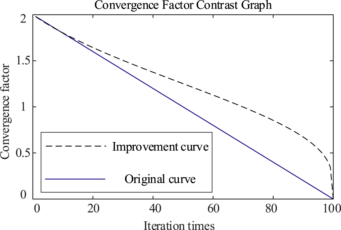
According to the comparison curve in Fig. 1, a higher convergence factor $\vec{a}$ declines in a non-linear manner as iterations increase, and the decline degree of $\vec{a}$ in the first and middle periods decreases, which effectively improves the global optimization, and the attenuation strength of $\vec{a}$ in the later periods increases, and it can accurately local optimization, such that it may successfully balance the skills of both local and global optimization.

Fig. 1

Convergence Factor Contrast Graph.

In the gray wolf algorithm, wolf l α is not optimal, which leads to wolf l ω approaching the local optimal in the iterative process. Weight modification is implemented to balance the capabilities of local search with global search. According to equation (34)–(36), obtain the proportional weight of the position: $\partial_{1} = {| X_{1} |}^{2} / (| X_{1} | | X_{1} | + | X_{2} | | X_{1} | + | X_{3} | | X_{1} |)$ (39) $\partial_{2} = {| X_{2} |}^{2} / (| X_{1} | | X_{2} | + | X_{2} | | X_{2} | + | X_{3} | | X_{2} |)$ (40) $\partial_{3} = {| X_{3} |}^{2} / (| X_{1} | | X_{3} | + | X_{2} | | X_{3} | + | X_{3} | | X_{3} |)$ (41)

Among them ∂₁, ∂₂, and ∂₃ correspond to the learning speed of three wolves l α, l β and lδ, respectively. Because the calculation of proportion weight includes the dynamic position change of three wolves, it has the role of position guidance. In this way, to successfully balance the capabilities of local and global search across algorithms and speed up convergence, ongoing dynamic adjustment is necessary. Finally, the iteration mode of adding weight proportion is as follows: $\vec{X} (t + 1) = (\partial_{1} {\vec{X}}_{1} + \partial_{2} {\vec{X}}_{2} + \partial_{3} {\vec{X}}_{3})$ (42)

The following measures may be taken to improve the GWO_SVM regression model in light of the study above:

Set the parameter limit and initialize the wolves, and the individual position is composed of r and C.

SVM trains samples according to r and C in individual positions, and tests individual fitness functions in SVM.

The updated GWO algorithm is utilized to update each wolf’s specific location. At the end of the hunting process, the best r and C are obtained and the best individual position is returned.

The r and C obtained by the improved GWO are utilized to create the model and do the analysis of the predictions.

Figure 2 depicts the flow chart for enhanced GWO_SVM wind power forecast based on the weighted composite index’s gray relation.

Fig. 2

Similar Days of Compound Indicators and Flow Chart of Improving GWO_SVM Wind Power Prediction.

3.3 Limitations of the proposed methods

The performance of the GWO_SVM method is intricately tied to the quality and accessibility of input data. Should the dataset incorporate noise or display missing values, this may lead to a diminishment in prediction accuracy. Consequently, this article undertakes a preprocessing step on NWP data to ameliorate the performance of GWO_SVM. However, intrinsic limitations persist due to the inherent characteristics of the SVM model itself.

Firstly, when confronted with extensive datasets, the GWO_SVM method may encounter constraints pertaining to computational resources, given the relatively time-intensive nature of SVM model training and optimization. Consequently, further optimization of computational time is warranted when conducting long-term wind power predictions.

Secondly, the GWO_SVM method may exhibit suboptimal performance in addressing highly nonlinear wind power prediction scenarios, as SVM inherently possesses restricted modeling capabilities for nonlinear data. Despite the integration of IGWO to enhance SVM, performance may still wane with larger datasets.

Furthermore, the generalization proficiency of the GWO_SVM method may be influenced by idiosyncratic datasets. Thus, judicious evaluation of its performance is imperative when extending the model’s application to diverse regions or distinct temporal intervals.

Lastly, if the distribution of newly acquired data markedly deviates from the training dataset, recalibration or retraining of the GWO_SVM model may be necessitated to uphold predictive accuracy.

In summation, notwithstanding the advantages exhibited by the GWO_SVM method in short-term wind power prediction, pragmatic application demands a nuanced consideration and resolution of the associated limitations.

4 Case analysis

This article uses 2018 wind farm data with NWP data to verify its conclusions. There is a 15-minute pause between samples. The 24 dynamic and thermodynamic indices produced by NWP are shown in Table 1. These indices include air pressure, wind direction, wind speed, cloud quantity, and precipitation. Evaluation indexes of prediction results: root mean squared error (RMSE), regression correlation coefficient (r²), mean absolute error (MAE) and mean absolute percent error (MAPE) in regression problems [35].

Table 1
Meteorological Index

Index Unit Index Unit

10 m Wind direction Deg Sea surface pressure Pa

30 m Wind direction Deg Surface pressure Pa

100 m Wind direction Deg Momentum flux W/m²

170 m Wind direction Deg Heat flux W/m²

Surface wind Deg Latent heat flux W/m²

10 m Wind speed m/s 2 m humidity %

30 m Wind speed m/s relative humidity %

100 m Wind speed m/s 1 s average wind speed m/s

170 m Wind speed m/s 1 s minimum wind m/s

Surface Wind speed m/s 1 s maximum wind m/s

Long wave radiation kJ/m² temperature K

Short wave radiation kJ/m² cloudiness

Index	Unit	Index	Unit
10 m Wind direction	Deg	Sea surface pressure	Pa
30 m Wind direction	Deg	Surface pressure	Pa
100 m Wind direction	Deg	Momentum flux	W/m²
170 m Wind direction	Deg	Heat flux	W/m²
Surface wind	Deg	Latent heat flux	W/m²
10 m Wind speed	m/s	2 m humidity	%
30 m Wind speed	m/s	relative humidity	%
100 m Wind speed	m/s	1 s average wind speed	m/s
170 m Wind speed	m/s	1 s minimum wind	m/s
Surface Wind speed	m/s	1 s maximum wind	m/s
Long wave radiation	kJ/m²	temperature	K
Short wave radiation	kJ/m²	cloudiness

Among these metrics, RMSE is calculated as the square root of the average of squared deviations between predicted and actual values, normalized by the sample size. It serves as a gauge for the disparity between predicted and observed values, exhibiting a high sensitivity to outliers within a set of forecasted values. Consequently, RMSE serves as a robust indicator of model precision. R-squared (r²), which delineates the proportion of variability in the dependent variable that the model accounts for, manifests superior regression performance with increasing values. It is derived by dividing the absolute error of each observation by its corresponding actual value, followed by computing the average. Meanwhile, MAE quantifies the average of absolute discrepancies, offering a reliable portrayal of the true magnitude of prediction errors. MAPE delineates the distinctions between predicted and actual values, with higher values signifying diminished predictive efficacy. $M A P E = \frac{1}{n} \sum_{i = 1}^{n} \frac{| S_{i} - Y_{i} |}{S_{i}} \times 100$ (43) $RMSE = \sqrt{\frac{1}{n} \sum_{i = 1}^{n} {(S_{i} - Y_{i})}^{2}}$ (44) $MAE = \frac{1}{n} \sum_{i = 1}^{n} | S_{i} - Y_{i} |$ (45) $r^{2} = (\frac{\sum_{i = 1}^{n} (S_{i} - \bar{S}) (Y_{i} - \bar{Y})}{\sqrt{\sum_{i = 1}^{n} (S_{i} - \bar{S})^{2}} \sqrt{\sum_{i = 1}^{n} (Y_{i} - \bar{Y})^{2}}})^{2}$ (46)

Where S is the real electricity generated by the wind; Y is the anticipated performance of wind power; $\bar{S}$ and $\bar{Y}$ is the average value.

Over two days, 192 sets of data, totaling 4608 data points, were carefully selected for a thorough analysis involving dimensionality reduction and visualization. The t-SNE method was employed to effectively reduce noise in the NWP sample set and provide an intuitive representation of weather sample characteristics in lower-dimensional spaces. This led to a reduction from the original 24-dimensional space to both two and three-dimensional subspaces, as illustrated in Fig. 3. Here, distinct colors signify different contributing factors, while individual points represent specific data points. Our analysis utilized a perplexity of 30, a learning rate of 500, and involved 1000 iterations. The application of the t-SNE algorithm resulted in a clear and discernible representation of all sample points in the two-dimensional space. Notably, the majority of samples displayed characteristic trajectories, demonstrating a consistent evolution even after perturbations. This observation highlights the temporal continuity and pulsatile nature inherent in weather variations.

Fig. 3

t-SNE visualization results. (a) The two-dimensional output of the t-SNE technique for dimensionality reduction. (b) The t-SNE technique produces a three-dimensional output for reducing dimensionality.

To assess the efficacy of dimensionality reduction techniques, both t-SNE and PCA were employed to reduce the training set data to two and three dimensions respectively. Table 2 presents the credibility results [36, 37], while Equation (49) defines the mathematical formulation for credibility. Credibility stands as a pivotal metric for assessing the preservation of local data structures post-dimensionality reduction. A higher level of credibility indicates a superior retention of data integrity following dimensionality reduction. The findings in Table 2 demonstrate that t-SNE, when utilized for low-dimensional representation, significantly enhances dimensional reliability compared to PCA. Additionally, t-SNE effectively preserves the temporal characteristics of the original data.

Table 2

Two-day data credibility calculation results

Method	2 Dimension	3 Dimension
t-SNE	0.9870	0.9947
PCA	0.9849	0.9908

$M 1 (k) = 1 - \frac{2 \sum_{i = 1}^{N} \sum_{x_{j} \in U_{k} (x_{i})} (r (x_{i}, x_{j}) - k)}{(Nk \cdot (2 N - 3 k - 1))}$ (47)

Where M1(k) ranges from 0 to 1. r(x_i,x_j) represents the rank of sample x_j sorted according to the distance from x_i in the original data space, and U_k(x_i) represents the set of adjacent data points k in the low dimensional space.

In the selection of training data based on the Grey Association, the time series data with the largest method is selected as the association sample. Figure 4 shows the two-day data association value view of WGRA and GRA. The entropy weight method yields a weight: Δ₁ = 0.7332, Δ₂ = 0.2668.

Figure 4 demonstrates that the data with a relation value of more than 0.5 accounts for around 35% of the total and the data with a relation value of more than 0.8 accounts for roughly 5% of the total. Because of the different conditions of relation, the data selection of the two methods has different effects. To compare the impact of training on data selection of WGRA and GRA, the selection conditions are defined as Ψ> 0.8and F > 0.8, respectively, so that the data with strong correlation can be retained as training parameters, and the data with weak correlation can be eliminated.

Fig. 4

Grey correlation results for two consecutive days.

In the short-term prediction analysis, the power output of the next day is predicted by taking 69120 data points of 2880 groups of data in 30 days as the training set. To demonstrate the good functionality of the suggested model (t-SNE_Weighted Composite GRA_IGWO Algorithm optimized SVM, t-SNE_WGRA_IGWO_SVM), this paper employs the t-SNE_ GRA_Improved Grey Optimization Algorithm optimized SVM (t-SNE_GRA _IGWO_SVM), t-SNE _IGWO_ SVM, IGWO_ SVM for comparison. Meanwhile, in order to more thoroughly assess the benefits of the enhanced gray wolf algorithm, the vector machine model based on ABC [38], GWO, PSO [39], and Genetic Algorithm (GA) [40] are established, which are t-SNE_WGRA_GWO_SVM, t-SNE_WGRA_ABC_SVM, t-SNE_WGRA_PSO_SVM, and t-SNE_WGRA_GA_SVM respectively. In order to forecast the production of wind energy, single back propagation neural network (BPNN) models have also been created.

Table 3 presents the initialization configurations for various methods. The parameter and error penalty ranges for kernel functions are specified as [0.01, 100]. These parameters are set to ensure uniformity in the number of iterations across algorithms, thus upholding the integrity of the comparison.

Table 3

The simulation parameters that are used by the algorithm for predictions

Methods	Parameters
IGWO algorithm optimized SVM	The number of iterations: 100; population number: 20
GWO algorithm optimized SVM	The number of iterations: 100; population number: 20
ABC algorithm optimized SVM	The number of iterations: 100; population number: 20
PSO algorithm optimized SVM	Population number: 20; the inertia weight is 1; the acceleration factor is 1.5 and 1.7; number of iterations: 100; SVM cross validation:3
GA algorithm optimized SVM	Catastrophe parameter: 0.01; catastrophe parameter: 0.01; catastrophe parameter: 0.01; crossover probability: 0.4; population number: 50;
BPNN	Learning rate:0.1; number of iterations: 300;

Table 4 displays a comparison of credibility results for PCA and t-SNE under different dimensionality reduction scenarios. The higher the credibility value of data, the more perfect the retention of data characteristics. At the same time, the lower the dimension, the smaller the calculation amount. t-SNE can also retain the feature value of data more completely in low-latitude data, so this paper selects two-dimensional data after t-SNE dimension reduction.

Table 4

30-day data credibility calculation results

Method	2 Dimension	3Dimension	7 Dimension
t-SNE	0.9902	0.9912	0.9964
PCA	0.9692	0.9878	0.9916

Figure 5 presents the visualization results of t-SNE dimensionality reduction. It is evident from Fig. 5 that, whether in two or three dimensions, the data exhibits a discernible classification effect. This observation suggests that even after dimensionality reduction, the continuity of NWP data may still be preserved within the dataset.

Fig. 5

Visualization results of t-SNE dimension reduction of 30 day data. (a) The two-dimensional output of the t-SNE technique for dimensionality reduction. (b) The t-SNE technique produces a three-dimensional output for reducing dimensionality.

Figure 6 shows the distribution of correlation values. The entropy weight method yields weights: Δ₁ = 0.5734, Δ₂ = 0.4266, and the training data selected by WGRA and GRA are about 5% of the total data.

Fig. 6

Visualization results of gray correlation between 30 day data and forecast days.

Figure 7 shows the predicted output waveform. Figure 7(a) shows that the single model BPNN and IGWO_SVM with no preprocessing data are poor in predicting wind power generation, which indicates that the single model can’t make good use of NWP data as training samples. In contrast, the prediction value of t_SNE_IGWO_SVM and t_SNE_BPNN methods are acceptable, but there are many weak association data, as the training sample of prediction, affects the accuracy of the forecast. Moreover, in training samples, WGRA outperforms GRA in terms of prediction impact. In addition, Fig. 7(b) shows that under the same data processing premise, IGWO has a better effect on SVM parameter optimization and a better prediction effect.

Fig. 7

The outcomes of making forecasts using a variety of models. (a) t-SNE_WGRA_IGWO_SVM, t-SNE_GRA_IGWO_SVM, t-SNE_IGWO_SVM, IGWO_SVM and BPNN; (b)t-SNE_WGRA_GWO_SVM, t-SNE_WGRA_ABC_SVM, t-SNE_WGRA_PSO_SVM and t-SNE_WGRA_GA_SVM models.

Table 5 presents a compilation of reductions in MAE, RMSE, and MAPE. As per equations (43) to (46), these numerical values offer a quantitative assessment of the accuracy and reliability of the algorithm’s predictions. With reference to the data provided in Table 5, the following conclusions can be drawn:

Table 5

One day wind power prediction results from different algorithms

Methods	MAPE	RMSE/%	MAE/%
t-SNE_WGRA_IGWO_SVM	7.611	4.98	4.09
t-SNE_GRA_ IGWO _SVM	8.3871	5.57	4.69
t-SNE_IGWO_SVM	9.379	5.78	4.82
IGWO_SVM	16.4608	16.36	13.31
t-SNE_WGRA_GWO_SVM	7.9912	5.01	4.5
t-SNE_WGRA_ABC_SVM	7.8919	4.98	4.1
t-SNE_WGRA_PSO_SVM	9.5611	3.39	2.32
t-SNE_WGRA_GA_SVM	14.694	9.45	5.48
BPNN	67.1234	19.53	10.43
t-SNE_BPNN	11.9532	7.59	5.33

The t-SNE_WGRA_IGWO_SVM model, which was suggested, obtains the greatest performance out of all of the other prediction models. Compared with t-SNE_GRA_IGWO_SVM and t-SNE_IGWO_SVM models, with reference to the assessment indices of MAE, RMSE, and MAPE, it can be discovered that the WGRA algorithm may reportedly enhance the capacity for anticipating the series of wind power production.

In comparison with t-SNE_IGWO_SVM and t-SNE_BPNN, the prediction performance of IGWO_SVM and BPNN models are worse, demonstrating that the t-SNE data preprocessing can better remove redundant features and prevent overfitting caused by too many features.

In parameter optimization, IGWO has better prediction performance than GWO. For instance, the MAE of t-SNE_WGRA_IGWO_SVM is 4.13, while the MAE of t-SNE_WGRA_GWO_SVM is 4.50. The upgraded IGWO model’s addition of the new convergence formula and iterative equation, which gives the IGWO model superior learning and generalization capabilities to quickly find the global optimum solution, maybe the main factor. Compared with other SVM optimization methods, on the premise of data preprocessing, the prediction results of all algorithms can have high accuracy. Meanwhile, the operation time of ABC, PSO, and GA is longer than that of IGWO. For the data in this paper, IGWO has better global performance and higher accuracy.

Making the findings more understandable, Table 6 lists the reductions in MAE, RMSE, and MAPE compared to models other than t-SNE_WGRA_IGWO_SVM. The correlation coefficient in Table 6 further demonstrates the superior performance of the suggested enhancement strategy.

Table 6

The reductions in MAE, RMSE, and MAPE compared to models other than t-SNE_WGRA_IGWO_SVM

Methods	MAPE	RMSE/%	MAE/%
t-SNE_GRA_ IGWO _SVM	9.25%	10.59%	12.79%
t-SNE_IGWO_SVM	18.85%	13.84%	15.14%
IGWO_SVM	53.76%	69.55%	69.27%
t-SNE_WGRA_GWO_SVM	4.75%	0.59%	9.11%
t-SNE_WGRA_ABC_SVM	3.55%	0	0.24%
t-SNE_WGRA_PSO_SVM	20.39%	–46.90%	–76.29%
t-SNE_WGRA_GA_SVM	48.20%	47.30%	25.36%
BPNN	88.66%	74.50%	60.78%
t-SNE_BPNN	36.32%	34.38%	23.26%

Additionally, Table 7 details the timespan needed to calculate data related to different approaches. The results in Table 7 show that single models, like BPNN, need much less time to run than their hybrid equivalents. However, hybrid models significantly outperform single models in terms of prediction accuracy. At the same time, without data preprocessing, including dimension reduction and association selection, the running time of the algorithm will be more burdened. For instance, IGWO_SVM takes quadruple as long to operate as t-SNE_WGRA_IGWO_SVM. Hence, in order to guarantee the reliability of the power system, it is acceptable to implement a way of producing wind power that is more precise and to devote sufficient time to the calculation process.

Table 7

Regression correlation coefficient r² of different algorithms and optimal SVM parameters

Methods	r ²	r/C	CPU/ s
t-SNE_WGRA_IGWO_SVM	0.9926	100/15.99	117.14s
t-SNE_GRA_ IGWO _SVM	0.9914	100/10.05	120.94s
t-SNE_IGWO_SVM	0.9902	17.42/26.96	363.63s
IGWO_SVM	0.9401	31.95/0.012	580.62s
t-SNE_WGRA_GWO_SVM	0.9914	100/9.56	120.79s
t-SNE_WGRA_ABC_SVM	0.9926	84.58/16.27	226.32s
t-SNE_WGRA_PSO_SVM	0.9959	100/100	2846.6s
t-SNE_WGRA_GA_SVM	0.9731	7.11/79.2	2246.7s
BPNN	0.9659	/	127.47s
t-SNE_BPNN	0.9950	/	38.27s

Table 8 provides a workload comparison between the proposed method and traditional approaches. The proposed method demonstrates notable contributions in data preprocessing, iterative process optimization, and data correlation analysis, thereby enhancing prediction accuracy in contrast to conventional methods. In the table, work1, work2, and work3 represent the work of data dimensionality reduction, iterative process optimization, and data correlation analysis, respectively.

Table 8

Comparison of workload between different methods

Methods	work1	work2	work3
t-SNE_WGRA_IGWO_SVM	√	√	√
t-SNE_GRA_ IGWO _SVM	√	×	×
t-SNE_IGWO_SVM	√	×	√
IGWO_SVM	×	×	√
t-SNE_WGRA_GWO_SVM	√	√	×
t-SNE_WGRA_ABC_SVM	√	√	×
t-SNE_WGRA_PSO_SVM	√	√	×
t-SNE_WGRA_GA_SVM	√	√	×
BPNN	×	×	×
t-SNE_BPNN	√	×	×

To illuminate the merits of our proposed methodology, we conducted Wilcoxon [41] and ANOVA analyses[42]. The former distinguished disparities in related or paired samples, while the latter ascertained potential differences in means across multiple groups. The Wilcoxon test, robust to non-normality, compared paired samples. In contrast, ANOVA evaluated differences in means among groups, assuming normality and variance homogeneity. Subsequently, both analyses were applied to forecasted and actual values from the proposed algorithm.

In the Wilcoxon analysis, a p-value of 0.66535 supported the null hypothesis, indicating favorable prediction accuracy. The ANOVA results (see Table 9 and Fig. 8) revealed non-significant differences between predicted and actual values (p = 0.7819 > 0.05), affirming the model’s accuracy. Where the sources of variance include Groups (between groups), Error (within groups), and Total (total); SS (Sum of squares) represents the sum of squares; df (Degree of freedom) represents the degree of freedom; MS (Mean squares) represents the mean square error; F represents the F value (F statistic). The F value is equal to the ratio of the mean square between groups and the mean square within the group, which reflects the random error. In summary, the proposed method demonstrates commendable predictive precision.

Table 9

One-way ANOVA

Source	SS	df	MS	F	Prob > F
Groups	0.0107	1	0.01071	0.08	0.7819
Error	26.4621	190	0.13927
Total	26.4728	191

Fig. 8

ANOVA analysis.

5 Conclusion and future directions

To enhance the precision and utility of wind power prediction models founded on NWP, this study introduces an integrated approach that combines NWP composite index grey correlation with an augmented GWO_SVM framework. For preprocessing NWP data, t-SNE is employed for dimensionality reduction and redundancy elimination, while the entropy weight technique is applied to compute data weights. These weights are then allocated to both the grey correlation degree and the simplified cosine similarity, thus constituting a novel composite index grey correlation for training data selection. Simultaneously, in recognition of the algorithm’s nonlinearity, we introduce a nonlinear convergence factor and an iterative method featuring dynamic proportion weight within the GWO. This strategic integration serves to harmonize local optimization capabilities with global search proficiency, expediting the optimization convergence process. Empirical findings substantiate that preprocessing data prior to predictions mitigates computational burden. Furthermore, optimization of data association procedures substantially amplifies prediction accuracy. Finally, augmenting the GWO algorithm markedly enhances the overall efficacy of wind power prediction. The effectiveness of this approach is substantiated through rigorous experimental scrutiny, providing valuable guidance for subsequent development of classification and regression models grounded in wind power time series data.

In recent years, notable progress has been made in both deep learning and reinforcement learning, resulting in significant breakthroughs across a multitude of domains. Within the realm of bionic intelligent algorithms, the integration of deep learning techniques has demonstrated pronounced efficacy in augmenting algorithmic convergence and dynamic iteration effects. Future research initiatives should emphasize the harmonious integration of deep learning and reinforcement learning methodologies, with the aim of refining the precision and responsiveness of wind power prediction models. This integrative approach holds substantial potential for advancing the capabilities of predictive models in the domain of renewable energy resources.

Declarations

Ethics approval Not applicable’ for that section.

Conflict of interest The Authors declare that there is no conflict of interest.

Author’s contributions All authors contribute equally to this manuscript.

Funding This work was supported by Ministry of Education University-Industry Cooperation Collaborative Education Project (202101301019;220602362291702); Zhanjiang University of Science and Technology Brand Enhancement Plan (PPJHKCSZ-2022278;PPJH2021009;PPJHYLKC-2022257).

References

Nejati

, Amjady

, Zareipour

, A New Multi-Resolution Closed-Loop Wind Power Forecasting Method, IEEE Transactions on Sustainable Energy (2023).

, He

, Zhang

, Kang

, Xia

, Bai

and Huang

, A short-term wind power forecasting approach with adjustment of numerical weather prediction input by data mining, IEEE Transactions on Sustainable Energy 6(4) (2015), 1283–1291.

Xiao

, Xu

, Xing

, Song

, Wang

and Zhao

, A federated learning system with enhanced feature extraction for human activity recognition, Knowledge-Based Systems 229 (2021), 107338.

Xing

, Xiao

, Qu

, Zhu

and Zhao

, An efficient federated distillation learning system for multitask time series classification, IEEE Transactions on Instrumentation and Measurement 71 (2022), 1–12.

Chen

, Ngai

E.W.

, Ku

, Xu

, Gou

and Zhang

, Prediction of hotel booking cancellations: Integration of machine learning and probability model based on interpretable feature interaction, Decision Support Systems 170 (2023), 113959.

Xiong

, Zha

, Qin

, Ouyang

and Xia

, Research on wind power ramp events prediction based on strongly convective weather classification, IET Renewable Power Generation 11(8) (2017), 1278–1285.

, Ensemble machine learning-based wind forecasting to combine NWP output with data from weather station, IEEE Transactions on Sustainable Energy 10(4) (2018), 2133–2141.

Hao

, Dong

, Liao

, Liang

, Wang

and Wang

, A novel clustering algorithm based on mathematical morphology for wind power generation prediction, Renewable Energy 136 (2019), 572–585.

Zhao

, Wang

, Liu

and Mechanical

S.O.

, Research on combination wind power forecasting based on gray correlation and cointegration theory, Acta Energiae Solaris Sinica 38(5) (2017), 1299–1306.

10.

Liu

, Jiang

, Zhang

and Niu

, A combined forecasting model for time series: Application to short-term wind speed forecasting, Applied Energy 259 (2020), 114137.

11.

Azad

H.B.

, Mekhilef

and Ganapathy

V.G.

, Long-term wind speed forecasting and general pattern recognition using neural networks, IEEE Transactions on Sustainable Energy 5(2) (2014), 546–553.

12.

, Luo

, Liu

, Cao

, Du

and Sun

, Wind power prediction based on EEMD-Tent-SSA-LS-SVM, Energy Reports 8 (2022), 3234–3243.

13.

Wang

, Wang

, Guo

, Hu

, Zhu

and Yu

, Multi-objective optimization of phase change cooling battery module based on optimal support vector machineoptimal support Vector Machine, Applied Thermal Engineering 236 (2024), 121386.

14.

Wang

, Zhang

, Kung

H.T.

, Johnson

V.C.

and Latif

, Extracting soil salinization information with a fractional-order filtering algorithm and grid-search support vector machine (GS-SVM) model, International Journal of Remote Sensing 41(3) (2020), 953–973.

15.

Huang

, Zhang

, Liu

, Zheng

and Wang

, A novel fault diagnosis system on polymer insulation of power transformers based on 3-stage GA-SA-SVM OFC selection and ABC-SVM classifier, Polymers 10(10) (2018), 1096.

16.

, Liu

, Chu

, Li

and Gu

, A disassembly sequence planning method with improved discrete grey wolf optimizer for equipment maintenance in hydropower station, The Journal of Supercomputing 79(4) (2023), 4351–4382.

17.

Mirjalili

, Mirjalili

S.M.

and Lewis

, Grey wolf optimizer, Advances in Engineering Software 69 (2014), 46–61.

18.

Dai

, Niu

and Li

, Daily peak load forecasting based on complete ensemble empirical mode decomposition with adaptive noise and support vector machine optimized by modified grey wolf optimization algorithm, Energies 11(1) (2018), 163.

19.

Liao

and Xu

, Approaches to manage hesitant fuzzy linguistic information based on the cosine distance and similarity measures for HFLTSs and their application in qualitative decision making, Expert Systems with Applications 42(12) (2015), 5328–5336.

20.

Ndiaye

and Gabriel

, Principal component analysis of the electricity consumption in residential dwellings, Energy and Buildings 43(2-3) (2011), 446–453.

21.

Lam

J.C.

, Wan

K.K.

, Cheung

K.L.

and Yang

, Principal component analysis of electricity use in office buildings, Energy and Buildings 40(5) (2008), 828–836.

22.

, Wang

, Xie

and Zhang

, Wind farm NWP data preprocessing method based on t-SNE, Energies 12(19) (2019), 3622.

23.

Van der Maaten

, Hinton,

, Visualizing data using t-SNE, Journal of Machine Learning Research 9(11) (2008).

24.

Liu

, Forrest

J.Y.L.

, Grey systems: theory and applications, Springer Science and Business Media (2010).

25.

Zhao

, Kang

, Guo

, Zhang

and Li

, Gray relational analysis optimization for coalbed methane blocks in complex conditions based on a best worst and entropy method, Applied Sciences 9(23) (2019), 5033.

26.

Kuo

, Yang

and Huang

G.W.

, The use of grey relational analysis in solving multiple attribute decision-making problems, Computers and Industrial Engineering 55(1) (2008), 80–93.

27.

Hamzaçebi

, Pekkaya,

, Determining of stock investments with grey relational analysis, Expert Systems with Applications 38(8) (2011), 9186–9195.

28.

Kumar

P.N.

, Rajadurai

and Muthuramalingam

, Multi-response optimization on mechanical properties of silica fly ash filled polyester composites using taguchi-grey relational analysis, Silicon 10 (2018), 1723–1729.

29.

Shi

, Ding

, Lee

W.J.

, Yang

, Liu

and Zhang

, Hybrid forecasting model for very-short term wind power forecasting based on grey relational analysis and wind speed distribution features, IEEE Transactions on Smart Grid 5(1) (2013), 521–526.

30.

Delgado

and Romero

, Environmental conflict analysis using an integrated grey clustering and entropy-weight method: A case study of a mining project in Peru, Environmental Modelling and Software 77 (2016), 108–121.

31.

, Liu

, Yao

and Yan

, The effect of sample size on the grey system model, Applied Mathematical Modelling 37(9) (2013), 6577–6583.

32.

Zhou

, Tao

, Chen

and Liu

, Intuitionistic fuzzy ordered weighted cosine similarity measure, Group Decision and Negotiation 23 (2014), 879–900.

33.

Verma

V.S.

, Bhardwaj

and Jha

R.K.

, A new scheme for watermark extraction using combined noise-induced resonance and support vector machine with PCA based feature reduction, Multimedia Tools and Applications 78 (2019), 23203–23224.

34.

Kamel

S.R.

, YaghoubZadeh

and Kheirabadi

, Improving the performance of support-vector machine by selecting the best features by Gray Wolf algorithm to increase the accuracy of diagnosis of breast cancer, Journal of Big Data 6 (2019), 1–15.

35.

Hanifi

, Liu

, Lin

and Lotfian

, A critical review of wind power forecasting methods— past, present and future, Energies 13(15) (2020), 3764.

36.

Kaski

, Nikkilä

, Oja

, Venna

, Törönen

and Castrén

, Trustworthiness and metrics in visualizing similarity of gene expression, BMC Bioinformatics 4(1) (2003), 1–13.

37.

, Wang

, Xie

and Zhang

, Wind farm NWP data preprocessing method based on t-SNE, Energies 12(19) (2019), 3622.

38.

, Li

and Li

, Performance evaluation of energy transition based on the technique for order preference by a similar to ideal solution and support vector machine optimized by an improved artificial bee colony algorithm, Energies 12(16) (2019), 3059.

39.

Zeng

, Qiu

, Wang

, Liu

, Zhang

and Li

, A new switching-delayed-PSO-based optimized SVM algorithm for diagnosis of Alzheimer’s disease, Neurocomputing 320 (2018), 195–202.

40.

Phan

A.V.

, Nguyen

M.L.

and Bui

L.T.

, Feature weighting and SVM parameters optimization based on genetic algorithms for classification problems, Applied Intelligence 46 (2017), 455–469.

41.

Serbet

, Kaya

, Statistical Analysis and EEG Signal Filtering Using Design of Window Function Based on Optimization Methods, Journal of Circuits, Systems and Computers (2023).

42.

Arfuso

, Minuti

, Liotta

, Giannetto

, Trevisi

, Piccione

and Lopreiato

, Stress and inflammatory response of cows and their calves during peripartum and early neonatal period, Theriogenology 196 (2023), 157–166.