Constructing prediction intervals to explore uncertainty based on deep neural networks

Abstract

The conventional approaches to constructing Prediction Intervals (PIs) always follow the principle of ‘high coverage and narrow width’. However, the deviation information has been largely neglected, making the PIs unsatisfactory. For high-risk forecasting tasks, the cost of forecast failure may be prohibitive. To address this, this work introduces a multi-objective loss function that includes Prediction Interval Accumulation Deviation (PIAD) within the Lower Upper Bound Estimation (LUBE) framework. The proposed model can achieve the goal of ‘high coverage, narrow width, and small bias’ in PIs, thus minimizing costs even in cases of prediction failure. A salient feature of the LUBE framework is its ability to discern uncertainty without explicit uncertainty labels, where the data uncertainty and model uncertainty are learned by Deep Neural Networks (DNN) and a model ensemble, respectively. The validity of the proposed method is demonstrated through its application to the prediction of carbon prices in China. Compared with conventional uncertainty quantification methods, the improved interval optimization method can achieve narrower PI widths.

Keywords

Prediction interval uncertainty prediction deep neural networks carbon price

1 Introduction

As an advanced technology, artificial intelligence has been developed rapidly, and it has achieved significant advancements in several domains recently, including autonomous driving [1, 2], medical diagnosis [3, 4], power load [5], finance [6 –8], and wind power generation [9 –11].

The majority of the predictions made thus far are point predictions with no uncertain information. The uncertainty arises from both aleatory (or data) uncertainty and epistemic (or model) uncertainty. Specially, aleatory uncertainty originates from unobserved explanatory variables, beyond those represented by x, or from inherently stochastic processes. Epistemic uncertainty arises from incomplete knowledge about the model, often due to the inherent imperfections of models. The enduring objectives of point prediction systems are high prediction accuracy and the removal of prediction errors. Nonetheless, the prediction error and uncertainty cannot be eliminated in practical application [12]. Although artificial intelligence has achieved high prediction accuracy, the information provided by point prediction is limited in the face of high-risk tasks. Once the prediction fails, it will carry a high level of risk, and moreover, it is not enough for forecast demanders to provide a definitive point forecast. Therefore, we need to provide forecasting reliability to offer more information; this requires us to quantify the uncertainty of the forecast. Compared to point prediction, a prediction interval directly expresses uncertainty by providing both a lower and an upper bound. This ensures that the actual values are likely to fall within these boundaries. The quality of prediction intervals is typically assessed quantitatively using metrics such as Prediction Interval Coverage Probability (PICP), Mean Prediction Interval Width (MPIW), and Coverage Width Criterion (CWC). PIs are more reliable and provide additional information for decision-makers, contributing to more rational decision-making processes.

At present, there are methods that generate PI, including delta [13], Bayesian [14, 15], mean-variance estimation (MVE) [16, 17], bootstrap [18, 19], quantile regression [20, 21], kernel density estimation method [22, 23], Gaussian process [24], and LUBE [25]. These methods can be divided into two categories according to whether they require a priori assumptions.

The first type of method includes PI constructed by the delta, Bayesian, MVE, and bootstrap, it assumes that the data follow some prior distribution, and then the lower and upper bounds of the interval can be calculated in which the data may fall at a given probability level [26]. However, these methods have non-negligible drawbacks. The delta requires a large amount of computation and cannot be effectively applied in practice; the Bayesian calculates PI with low accuracy and requires a lot of computation because each parameter has a predetermined distribution; the MVE produces a small coverage of PI; and the bootstrap method is demanding and time-consuming for computing devices. Moreover, the approaches mentioned above make use of distributional assumptions that are constructed based on a priori knowledge or prediction errors; nevertheless, it is not always possible to guarantee that these distributional assumptions are accurate.

The second type of method includes quantile regression, kernel density estimation, and Gaussian processes, which are not constrained by the assumption distribution of data and prediction error, and we can construct PIs directly for uncertainty. Their core idea is to train a model by minimizing an error-based loss function, and then use the output of the trained model to construct PI. However, these methods rely on point prediction and have difficulty handling high-dimensional and massive data.

To solve the aforementioned issue, A. Khosravi et al. [25] introduced a new method for constructing PI based on a single-layer feedforward neural network that can output lower and upper bounds directly; this method is known as LUBE. Because the parameters used by the method to form the cost function of the training network are the same as those used to assess the quality of the generated PI, the computational effort is minimal. It provides PIs with a high coverage probability and small average width without assuming any data distribution [27]. Although the LUBE approach has achieved widespread popularity, it still has some defects that limit the accuracy development of interval prediction to some degree. Firstly, the loss function is non-differentiable, making optimization challenging. As training approaches, only non-gradient algorithms can be employed. However, gradient descent (GD) is the standard method for training neural networks. Second, because the LUBE loss function is defined by PI characteristics, it lacks statistical significance and achieves a global optimum only when the PI’s width is zero. Furthermore, the method simply accounts for the data noise variance and does not explain the model uncertainty. T. Pearce et al. [28] developed a loss function that can be utilized with GD and does not require distributional assumptions to address these flaws. The model uncertainty is taken into account in ensemble form. Salem et al. [29] introduced a multi-objective loss function that incorporates PIs and point estimations based on T. Pearce, and their incorporated penalty function enhances the semantic integrity of the results and stabilizes the training process of the network. In addition, it aggregates the set PIs into a split-normal mixture such that the PIs capture aleatory uncertainty and epistemic uncertainty. N. Rosenfeld et al. [30] proposed a discriminating learning framework for optimizing the expected error rate with interval-size budget constraints. In the framework of batch learning, PIs for a set of test points can be constructed simultaneously. Y. Lai et al. [31] integrated the MPIW into the form of the negative log-likelihood (NLL) as an estimate of the uncertainty. It makes the width of the constructed PI closely related to uncertainty.

The above works have largely contributed to the development of uncertainty prediction. Nevertheless, the deviation of the forecast target value from the forecast interval was not considered in previous research, which is a problem that cannot be ignored and, to some extent, limits the improvement of the forecast interval accuracy. In this work, a novel multi-objective loss function that further considers the accumulative deviation of the PI is built based on earlier works. First, the new loss function incorporates PIs and point estimates. Second, the width of the PI is closely related to uncertainty. In addition, the accumulative deviation of the PI is introduced by the loss function, which can lower the prediction risk. In this study, DNNs with robust learning capabilities are employed to build trustworthy PIs by implicitly learning uncertainty within the LUBE framework under the guidance of loss functions.

The majority of carbon price forecasting techniques examined in the literature to date are point predictions[32 –36], and few uncertainty forecasts about carbon price are made. We try to use the created approach to predict the PI of carbon price. In contrast to previous research on time series forecasting of carbon price, this study considers multiple factors affecting carbon prices for multivariate regression forecasting. Moreover, a variable filtering procedure was used to remove variables with low correlation, thereby reducing redundant work.

The contributions of this study include:

An improved PI optimization framework is established by introducing the optimization objective of PI deviation information in the loss function, which provides a new idea for optimizing PIs.

This study combines the LUBE technique with deep learning models. Guided by the loss function, the DNN uses the LUBE framework to directly estimate the PI.

A new carbon price forecasting framework that provides more information on carbon price uncertainty is proposed. This study enriches the research on carbon price forecasting, and PI can provide more comprehensive information to policymakers.

The rest of this paper is structured as follows: Section 2 describes the process of PI construction, and shows the prediction process of the proposed method. Section 3 presents the data selection process and the evaluation metrics of the PIs. Section 4 presents the procedure of the experiment and discusses the results. Section 5 summarizes the whole paper and points out the direction of future work.

2 Construction of the optimal PI for uncertain estimation

In this part, a LUBE-based quantified uncertainty approach for building PI in deep neural networks is provided; this model is called LUBE-PIAD-DNN. This section details the construction principle of the optimized loss function introduced into PIAD and also shows the theoretical and predictive process of LUBE-PIAD-DNN to generate PI.

2.1 The uncertainty framework

The principle of regression is to apply the data generation function f (x) in combination with additional noise to express the observable target value y:

In general, the goal of regression is to generate a function $\hat{f} (x)$ that predicts the point estimate. However, additional terms must be evaluated to estimate the uncertainty of y. It is assumed that both components of Equation (1) have associated sources of uncertainty, which correspond to the uncertainty in model and the uncertainty in data, respectively. The two terms that make up the observations’ total variance, assuming that they are independent, are as follows:

$y = f (x) + σ_{noise},$ (1) where σ_noise is referred to as irreducible noise or data noise, its presence may come from unobserved explanatory variables in addition to x or inherently stochastic processes.

$σ^{2} = σ_{model}^{2} + σ_{data}^{2},$ (2)

is the source of model uncertainty or epistemic uncertainty, epistemic uncertainty arises from incomplete knowledge about the model, often due to the inherent imperfections of models. Whereas is the source of data uncertainty or aleatory uncertainty.

We assume that the size of a mini-batch is n, and x_i is the i - th input of y_i. The principle of uncertainty quantification is to predict a PI $[{\hat{y}}_{Li}, {\hat{y}}_{Ui}]$ , This PI limits y_i in such a way that:

$PICP = \frac{1}{n} \sum_{i = 1}^{n} c_{i},$ (4) where c_i = 1 if y_i is within the interval $[{\hat{y}}_{Li}, {\hat{y}}_{Ui}]$ , otherwise c_i = 0. It is important to note that although Equation (3) is always met, such a PI is meaningless when ${\hat{y}}_{Li}$ is extremely small and ${\hat{y}}_{Ui}$ is sufficiently large. The ideal PI should be as narrow as possible and satisfy Equation (3).

MPIW stands for the mean PI width [25,28,31,37 , 25,28,31,37], which is defined as:

$Pr [{\hat{y}}_{Li} ⩽ y_{i} ⩽ {\hat{y}}_{Ui}] ⩾ P_{c},$ (3) where $Pr [{\hat{y}}_{Li} ⩽ y_{i} ⩽ {\hat{y}}_{Ui}]$ is the PI coverage probability (PICP), P_c is the predefined confidence level. It is a spontaneous measurement correlated with the created PI’s credibility and is represented as:

$MPIW = \frac{1}{n} \sum_{i = 1}^{n} ({\hat{y}}_{Ui} - {\hat{y}}_{Li}) .$ (5)

2.2 The loss function of uncertainty-based PI (UBPI)

Y. Lai et al. [30] have shown that their method of interval prediction outperforms Quantile Regression (QR) [38], Gradient Boosting Decision Tree with Quantile Loss (QR_GBDT) implemented in the Scikit-learn package [39], the quality-based PI construction method IntPred [40], Quality Driven Ensemble (QD-Ens) [28], and the prediction interval aggregation method SNM [28]. In the Y. Lai et al. [30] study, the loss function of uncertainty-based PI(UBPI) is defined with two terms:

$L = L_{MPIW} + λ_{1} L_{PI},$ (6) where $L_{MPIW}$ represents the loss of PI width and point estimate, $L_{PI}$ denotes the loss of PI coverage probability. λ₁ is the hyper-parameter that balances the importance of two terms.

We derive the $L_{MPIW}$ by estimating the uncertainty in the regression task. The regression likelihood combined with the probability density function of the Gaussian distribution yields the NLL of the regression [25, 41], as follows:

The $L_{MPIW}$ is defined by the following equation after we simplify Equation (7):

$\begin{matrix} NLL = - \sum_{i = 1}^{n} log [\frac{1}{\sqrt{2 π} σ} exp (- \frac{(y_{i} - {\hat{y}}_{i})^{2}}{2 σ^{2}})] \\ = \frac{n}{2} [\frac{\frac{1}{n} \sum_{i = 1}^{n} (y_{i} - {\hat{y}}_{i})^{2}}{σ^{2}} + log (σ^{2}) + log (2 π)], \end{matrix}$ (7) where σ² represents the uncertainty of the output. In Equation (7), MPIW is used in place of σ². The interval width is considered a good indicator of uncertainty. The uncertainty increases as the interval widens. Conversely, the narrower the interval, the smaller the uncertainty.

$\begin{matrix} L_{MPIW} = \frac{n}{2} [\frac{\frac{1}{n} \sum_{i = 1}^{n} (y_{i} - {\hat{y}}_{i})^{2}}{σ^{2}} + log (σ^{2})] \\ \approx \frac{n}{2} [\frac{MSE}{MPIW} + log MPIW], \end{matrix}$ (8) where MSE is the mean squared error of a mini-batch, and we use the midpoint of interval as the point estimation.

${\hat{y}}_{i} = \frac{{\hat{y}}_{Li} + {\hat{y}}_{Ui}}{2},$ (9)

$MSE = \frac{1}{n} \sum_{i = 1}^{n} (y_{i} - {\hat{y}}_{i})^{2}$ (10)

The $L_{MPIW}$ loss consists of a residual regression term and an uncertainty regularization term. We implicitly learn data uncertainty from the loss function without requiring uncertainty labels. The network is prevented from producing too many large and nonsensical PIs by the second regularization term [31].

Studies [25, 28] provide inspiration for $L_{PI}$ , which is developed as follows to learn the PI:

$L_{PI} = [max (0, P_{c} - PICP)]^{2}$ (11)

Equation (11) implies that PICP will be penalized during the training process if it is less than a predetermined confidence level P_c. That is, PICP should be greater than or equal to P_c to avoid the penalty.

The Boolean c_i in Eq. (4) results in the $L_{PI}$ loss that is non-differentiable for the backpropagation method because of the operation max in Eq. (11). Therefore, we also replace c_i with a softened version, as shown below, based on earlier research [28 , 43].

$c_{i} = f_{sigmoid} (s \cdot ({\hat{y}}_{Ui} - y_{i})) \cdot f_{sigmoid} (s \cdot (y_{i} - {\hat{y}}_{Li})),$ (12) where f_sigmoid is the sigmoid activation function and s > 0 is the hyper-parameter factor of softening.

The loss function of UBPI is defined as:

$\begin{matrix} {Loss}_{UBPI} = \frac{n}{2} [\frac{MSE}{MPIW} + log MPIW] \\ + λ_{1} {[max (0, P_{c} - PICP)]}^{2}, \end{matrix}$ (13) where n is the number of predicted y. λ₁ balances the importance between PICP and MPIW.

2.3 The loss function of the proposed LUBE-PIAD-DNN

To the best of our knowledge, only the loss of width and coverage has been considered in the existing literature, while the loss of deviation information has not been taken into account, which would make the effectiveness of PI somewhat compromised. Based on the work of Y. Lai et al. [30], the PIAD optimization objective is introduced into the loss function. For the uncertainty to be quantified and the best PI to be provided, the loss function $L_{Total}$ is defined with three terms:

$L_{Total} = L_{MPIW} + λ_{1} L_{PI} + λ_{2} L_{PIAD} .$ (14)

$L_{PIAD}$ is the loss of the accumulative deviation of PI. These three penalty terms’ relative weights are balanced by the hyper-parameters λ₁ and λ₂. L_PIAD is used to measure the degree of deviation of forecast target values from the forecast interval. The deviation from PI for the i-th prediction point is defined as:

${PIAD}_{i} = {\begin{matrix} {\hat{y}}_{Li} - y_{i}, y_{i} ⩽ {\hat{y}}_{Li} \\ 0, {\hat{y}}_{Li} < y_{i} < {\hat{y}}_{Ui} \\ y_{i} - {\hat{y}}_{Ui}, y_{i} ⩾ {\hat{y}}_{Ui} \end{matrix}$ (15)

PIAD is defined as:

$PIAD = \sum_{i = 1}^{n} {PIAD}_{i},$ (16) where PIAD is the accumulative deviation between the actual values that fall outside the forecast interval and the forecast interval boundary. If both the width and coverage of PI are the same, the quality of PI is higher when the PIAD is small. The process of constructing the hybrid loss function is presented in Algorithm 1.

Table 1

Algorithm 1 Construction of hybrid loss function
Input: Target values y_i, predictions of lower bound ${\hat{y}}_{Li}$ and upper bound ${\hat{y}}_{Ui}$ , the confidence level Pc, sigmoid softening factor s, the hyper-parameters λ₁ and λ₂ balance the importance of three terms, the size of a mini-batch n, and the activation function σ.
Output: Loss $L_{Total}$
${\hat{y}}_{i} = ({\hat{y}}_{Li} + {\hat{y}}_{Ui}) / 2$ ;
$MSE = reduce_mean (y_{i} - {\hat{y}}_{i})^{2}$ ;
$MPIW = reduce_mean ({\hat{y}}_{Ui} - {\hat{y}}_{Li})$ ;
$c_{i} = f_{sigmoid} (s \cdot ({\hat{y}}_{Ui} - y_{i})) \cdot f_{sigmoid} (s \cdot (y_{i} - {\hat{y}}_{Li}))$ ;
PICP = reduce _ mean (c_i);
$L_{MPIW} = \frac{n}{2} [\frac{MSE}{MPIW} + log MPIW]$ ;
$L_{PI} = {[max (0, P_{citsc} - PICP)]}^{2}$ ;
${PIAD}_{i} = {\begin{matrix} {\hat{y}}_{Li} - y_{i}, y_{i} ⩽ {\hat{y}}_{Li} \\ 0, {\hat{y}}_{Li} < y_{i} < {\hat{y}}_{Ui} \\ y_{i} - {\hat{y}}_{Ui}, y_{i} ⩾ {\hat{y}}_{Ui} \end{matrix}$ ;
$L_{PIAD} = reduce_s um ({PIAD}_{iitsc})$ ;
$L_{Total} = L_{MPIW} + λ_{1} L_{PI} + λ_{2} L_{PIAD}$ .

Finding a fundamental equilibrium between the coverage probability and width of PI is the focus of recent research on the loss function of PI [25]. Recently, Y. Lai et al. [30] make the width of PI and uncertainty have a close link and verify that the method based on Loss_UBPI outperforms the state-of-the-art methods [28 , 38–40] at the time in terms of PI quality.

The loss function for the [24] is

$\begin{matrix} {Loss}_{LUBE} \\ = \frac{MPIW}{r} (1 + exp (λ_{1} max (0, P_{c} - PICP))), \end{matrix}$ (17) where r is the range of values of y_i.

The loss function of [28] is

$\begin{matrix} {Loss}_{SNM} = (1 - λ_{3}) (1 - λ_{4}) \cdot MPIW \\ + λ_{3} (1 - λ_{4}) \cdot max (0, P_{c} - PICP)^{2} \\ + λ_{4} \cdot MSE + ξ \cdot \frac{1}{n} \sum_{i = 1}^{n} [\begin{matrix} max (0, {\hat{y}}_{Ui} - {\hat{y}}_{i}) \\ + max (0, {\hat{y}}_{i} - {\hat{y}}_{Li}) \end{matrix}] . \end{matrix}$ (18) where λ₃, λ₄, ξ are hyperparameters that balance the different losses.

Inspired by [25] and [28–29 , 31], the proposed approach builds on them, and the case of prediction deviation information is further considered. As a result, while obtaining a “high coverage and narrow width” prediction interval, even if the forecast fails, the predicted value will still be as close to PI as possible. The advantages of the loss function constructed in this study have two aspects. First, both point estimates and PI are incorporated into this loss function. Second, the uncertainty is learned without requiring uncertainty labels.

Fig. 1

The basic structure of deep neural network.

Table 1

Parameter settings

Model	Parameters	Value
DNN	Number of layers	4
	Number of neurons in each layers	24,16,8,2
	Activation function	ReLU
	optimizer	Adam
	Batch size	16
	Epoch size	100
ANN	Number of layers	2
	Number of neurons in each layers	24,2
	Activation function	ReLU
	optimizer	Adam
	Batch size	16
	Epoch size	100
ELM	Number of layers	2
	Number of neurons in each layers	24,2
	Activation function	ReLU
	optimizer	Adam
	Batch size	16
	Epoch size	100
GRNN	Number of layers	2
	Number of neurons in each layers	50,2
	optimizer	Adam
	Batch size	16
	Epoch size	100
Loss function	λ₁, λ₂, λ₃, λ₄, P_c, s, ξ	0.5,0.005,0.9,0.8, 0.9,10,120

2.4 Deep neural network-based prediction interval model

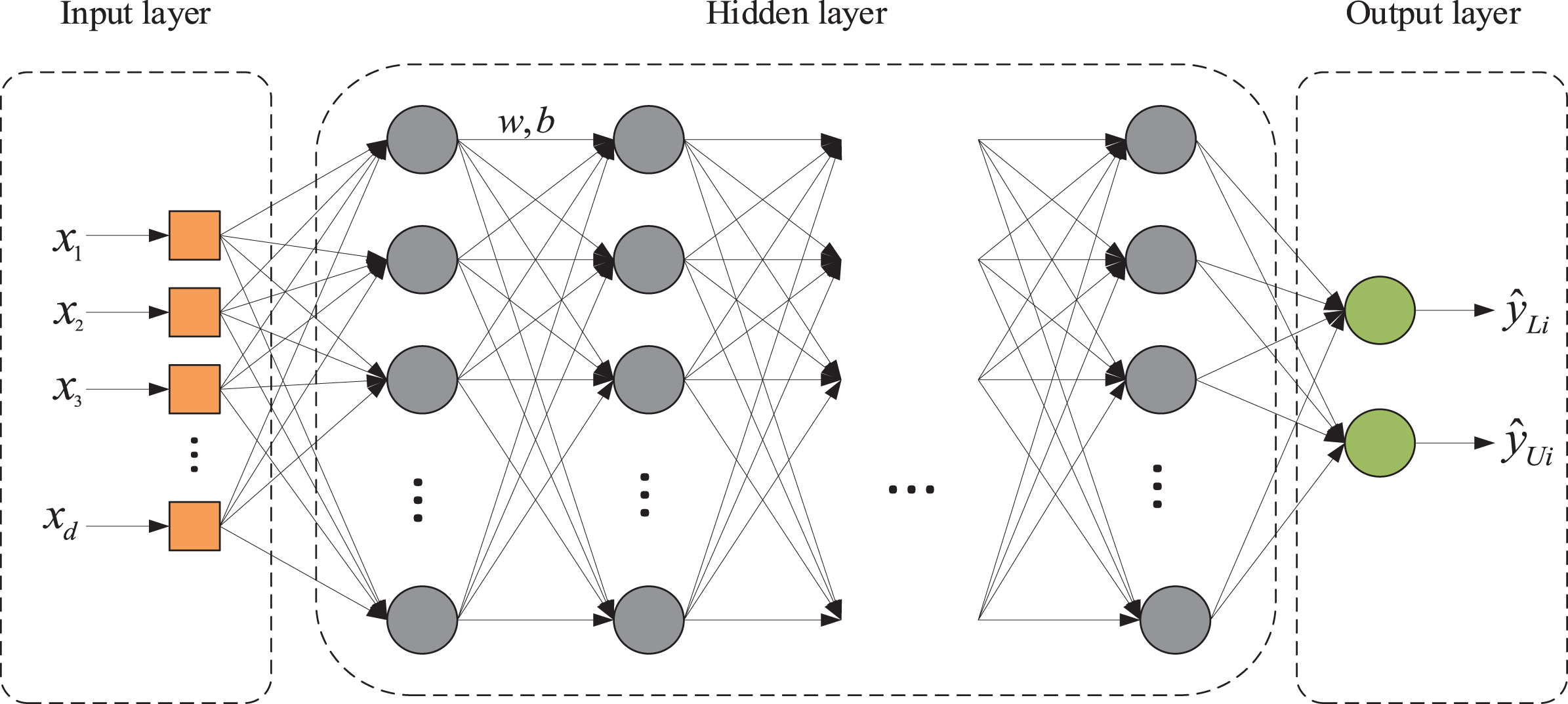
Deep neural networks are multilayer neural networks built on the basis of artificial neural networks (ANNs), where the more hidden layers there are, the more extensive the connections between neurons are. This makes it possible for autonomous learning to have more complex hidden features, which enhances DNN’s capacity to handle nonlinear problems in a range of domains. The DNN structure is shown in Fig. 1 and is made up of an input layer, many hidden layers, and an output layer, each of which uses the output of the layer before it as its input. w and b stand for the weight coefficient matrix and bias vector between layers, respectively, and x₁, x₂, ⋯ , x_d are the DNN’s inputs, ${\hat{y}}_{Li}$ , ${\hat{y}}_{Ui}$ are the DNN’s outputs.

2.5 Parameter setting and prediction process

In the experiment, the historical data of each carbon price series and the corresponding variables selected by MI-MRMR are used as inputs. The upper and lower bounds of the prediction interval are directly outputted using the machine learning-based LUBE-PIAD framework. After repeated trials, the parameters of the loss function and the neural network settings are shown in Table 1.

The prediction process is displayed in Fig. 2, and the specific steps are shown below.

Step 1. Collecting data. Data on carbon price and influencing factors are collected.

Fig. 2

The prediction process of the PI by DNN.

Step 2. The main variables that influence carbon prices are selected from a preliminary selection of 15 variables using variable selection methods.

Step 3. Data processing. The sample is divided into two sets: training and testing, and all data are normalized.

Step 4. Training the deep neural network. The training data are input into a deep neural network with a loss function of $L_{Total}$ . Until the maximum number of iterations is reached and the following criteria are satisfied, the deep learning network training is complete, which means that the prediction model is created. The created model can be used to directly provide prediction intervals $[{\hat{y}}_{Li}, {\hat{y}}_{Ui}]$ . For each interval, the smaller value is ${\hat{y}}_{Li}$ , and the greater value is ${\hat{y}}_{Ui}$ .

$\begin{matrix} min L_{Total} = L_{MPIW} + λ_{1} L_{PI} + λ_{2} L_{PIAD}, \\ s . t . PICP ⩾ P_{c} . \end{matrix}$ (19)

Fig. 3

The trading volume of China’s carbon market.

Step 5. Testing the deep neural network. Prediction intervals are produced directly by feeding test data into the trained deep neural network for prediction.

Step 6. Generating the final prediction interval. The final prediction interval is generated in the form of an ensemble. The ensemble concept, which we employ, is straightforward but effective. The ensemble model consists of several LUBE-PIAD-DNNs with different initial parameters [30]. In the process of prediction, for the randomness of the model predictions to be removed and the uncertainty of the model to be learned, the whole training and testing model is repeated 30 times, and the upper and lower bounds of the forecasts are then averaged, respectively. The average value represents the upper and lower bounds of the final PI.

${\tilde{y}}_{Li} = \frac{1}{m} \sum_{j = 1}^{m} {\hat{y}}_{{Li}_{j}}$ (20)

${\tilde{y}}_{Ui} = \frac{1}{m} \sum_{j = 1}^{m} {\hat{y}}_{{Ui}_{j}},$ (21) where ${\hat{y}}_{Li}$ and ${\hat{y}}_{Ui}$ are the lower and upper bounds of the final PI, respectively, and m is the prediction times.

3 Experiment data

3.1 Selection and description of data

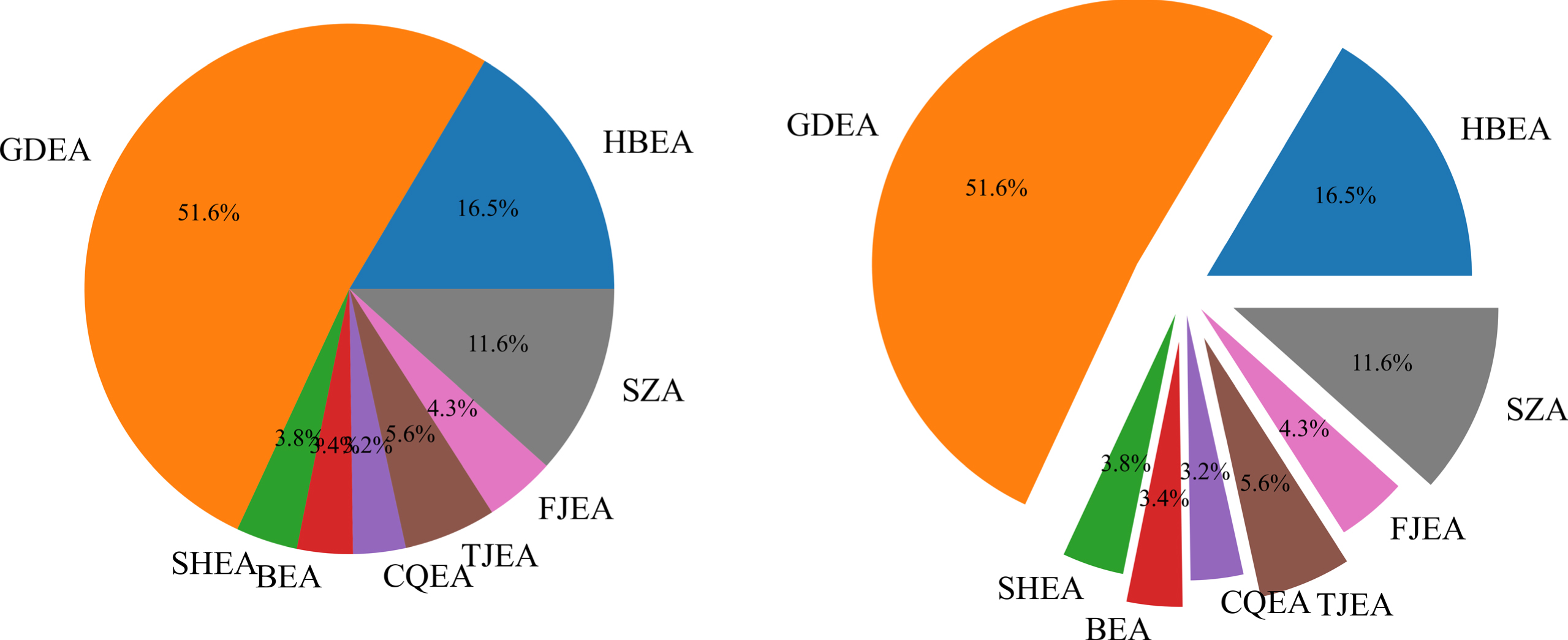
Data on China’s carbon price will be used for the empirical analysis. China has now established eight pilots for carbon trading, namely Hubei carbon market carbon emission allowance (HBEA), Guangdong carbon market carbon emission allowance (GDEA), Shenzhen carbon market carbon emission allowance (SZEA), Shanghai carbon market carbon emission allowance (SHEA), Beijing carbon market carbon emission allowance (BEA), Chongqing carbon market carbon emission allowance (CQEA), Fujian carbon market carbon emission allowance (FJEA), and Tianjin carbon market carbon emission allowance (TJEA). The activity and stability of carbon trading pilots through trading volume and market liquidity are discussed in this section. Finally, the carbon price of HBEA, GDEA, SZEA, and SHEA is selected as the object of empirical analysis.

The trading volume of China’s different carbon markets is shown in Fig. 3. Carbon markets in Guangdong, Hubei, and Shenzhen are the top three in trading volume within the sample interval, accounting for 51.2%, 16.3%, and 11.5% of all pilot trading volume, respectively. The larger trading volume indicates a more active and representative carbon market.

The ratio of trading days in different carbon markets is exhibited in Table 2. Hubei, Guangdong, Shenzhen, and Shanghai have carbon market ratios that are greater than 60% within the sample interval (95.19%, 94.57%, 86.93%, and 60.24%, respectively). High ratios indicate good liquidity and activity in these four markets.

Table 2
The ratio of trading days in different carbon markets

Carbon trading products The ratio of trading days Carbon trading products The ratio of trading days

HBEA 95.19% BEA 55.59%

GDEA 94.57% CQEA 53.62%

SZEA 86.93% FJEA 50.47%

SHEA 60.24% TJEA 24.39%

Carbon trading products	The ratio of trading days	Carbon trading products	The ratio of trading days
HBEA	95.19%	BEA	55.59%
GDEA	94.57%	CQEA	53.62%
SZEA	86.93%	FJEA	50.47%
SHEA	60.24%	TJEA	24.39%

Table 3

Factors affecting the carbon price

Influencing factors	Variable name	Data source
Carbon price	Hubei emission allowance	Wind
	Guangdong emission allowance
	Shenzhen emission allowance
	Shanghai emission allowance
Macroeconomy	USD/CNY exchange rate (x₁)	Investing.com
	EUR/CNY exchange rate (x₂)
	Shanghai securities composite index (x₃)
International carbon market	EUA futures carbon price (x₄)	Wind
Energy price	Rotterdam coal futures price (x₅)	Investing.com
	Brent crude oil futures price (x₆)
	WTI crude oil futures price (x₇)
	Gas price (x₈)
	Qinhuangdao steam coal 5500 (x₉)	Wind
	Daqing crude oil (x₁₀)
	The China LNG ex-works price national index (x₁₁)
Climate and the environment	Maximum air temperature (x₁₂)	Wind
	Minimum air temperature(x₁₃)
	Air quality index (AQI) (x₁₄)
Public attention	“Carbon emissions trading” Baidu index (x₁₅)	Index.baidu.com

To more comprehensively validate the performance of the LUBE-PIAD-DNN, an empirical analysis is being conducted on four active and two inactive carbon trading price datasets. The sample period spans from January 1, 2017, to February 28, 2022.

3.2 Description and basic statistics of variables

With reference to the reference [44] on the selection of variables affecting carbon price, 15 pertinent variables that may affect changes in carbon price in terms of macroeconomics, international carbon markets, energy prices, climate and environment, and public attention are selected in this study. The specific variables and data sources are shown in Table 3.

3.3 Evaluation Metrics for PI

To verify the effectiveness of the proposed method, we evaluate the quality of PI in terms of PICP, MPIW, and the coverage width criterion (CWC). PICP and MPIW are defined as shown in Equations (4), and (16) above, respectively, and CWC is defined as follows.

The PI normalized average width (PINAW) is designed by:

$PINAW = \frac{1}{nR} \sum_{i = 1}^{n} ({\hat{y}}_{Ui} - {\hat{y}}_{Li}),$ (22)

The CWC combines the coverage and width of the PI, which is defined as:

\begin{matrix} CWC = \\ {\begin{matrix} PINAW, PICP ⩾ P_{c} \\ PINAW (1 + γ (PICP) e^{(- η (PICP - P_{c}))}), PICP < P_{c} \end{matrix}, \end{matrix}

(23) }∥

γ (PICP) = {\begin{matrix} 0, PICP ⩾ P_{c} \\ 1, PICP < P_{c} \end{matrix},

(24) where

R = \max (y_{U i}) - \min (y_{L i})

is the range of the PI, and η is the penalty coefficient, which is used to penalize the case when PICP is smaller than P_c. If the PICP is smaller than the P_c, the prediction model will apply an exponential penalty to γ (PICP) to narrow the gap between the PICP and the P_c. The evaluation indications are primarily focused on PINAW when PICP is greater than or equal to P_c.∥

Table 4

Comparison of different variable screening methods

Carbon price	Variable selection method	Variables	PICP	MPIW	CWC
HBEA	MI	x₁, x₄, x₅, x₉, x₁₁	0.959	35.352	0.425
	RF	x₁, x₄, x₅, x₇, x₉	0.988	37.902	0.705
	MI-MRMR	x₄, x₅, x₆, x₁₄, x₁₅	0.988	11.766	0.311
	CC	x₄, x₅, x₆, x₉, x₁₀, x₁₁	0.955	35.928	0.623
	RFE	x₁, x₂, x₆, x₇, x₁₀	0.938	40.704	0.451
GDEA	MI	x₂, x₄, x₅, x₇, x₉	0.904	60.193	0.753
	RF	x₄, x₅, x₆, x₈, x₁₀	0.942	67.006	0.589
	MI-MRMR	x₁, x₄, x₅, x₈, x₁₅	0.925	39.117	0.538
	CC	x₁, x₄, x₅, x₆, x₉, x₁₀, x₁₁, x₁₅	0.933	66.525	0.857
	RFE	x₂, x₃, x₄, x₇, x₁₀	0.913	64.284	0.771
SZEA	MI	x₁, x₃, x₄, x₅, x₇	0.986	45.418	0.741
	RF	x₄, x₇, x₈, x₁₀, x₁₁	1	42.473	0.711
	MI-MRMR	x₂, x₄, x₁₃, x₁₄, x₁₅	0.932	25.185	0.505
	CC	x₄, x₆, x₁₀	0.996	95.043	0.996
	RFE	x₁, x₂, x₆, x₁₀, x₁₃	1	43.669	0.722

Note: The best value for each MPIW and CWC is shown in bold.

∥PICP reflects the reliability of PI, which indicates the probability that the prediction target falls into PI. MPIW reflects PI accuracy, the smaller the MPIW, the higher the PI’s accuracy degree. CWC is an evaluation metric that takes into account the PI’s coverage and width, the lower the CWC, the higher the PI’s quality.∥

3.4 Filtering of variables

To improve the efficiency of subsequent predictions, the initially determined 15 variables are screened. Firstly, main variables for HBEA, GDEA, and SZEA are chosen using Mutual Information (MI) [47], Random Forest (RF) [48], Recursive Feature Elimination (RFE) [49], Correlation Coefficient (CC) [45–46], and Mutual Information-based Maximum Relevance Minimum Redundancy (MI-MRMR) [50] method, respectively. Variables with a Correlation Coefficient greater than 0.3 are chosen, while other methods aim to select the top 5 variables. Then, the LUBE-PIAD-DNN predicts based on the selected variables. The prediction results using different selection methods are shown in Table 4. The most suitable variable selection method is determined based on PICP, MPIW, and CWC. PICP assesses only one aspect of prediction intervals. According to the principles of high-quality prediction intervals, if a prediction intervals meets the requirements, then the width of the prediction intervals will be given more consideration. It can be easily observed that the MI-MRMR method has an absolute advantage in effectively selecting variables. All PICPs meet the predetermined Pc. While, the prediction intervals derived from variable selection using the MI-MRMR method show significantly lower values in MPIW and CWC compared to those obtained through other methods. Particularly in the case of HBEA, under the condition where all PICPs are greater than 0.9, the MPIW obtained by MI-MRMR is 11.766, which is 23.559 smaller than the 35.325 achieved by the best comparative method. Among the comparative methods, MI performs the best, yet it is still significantly inferior to MI-MRMR, which demonstrates the good performance of mutual information-based feature screening. Hence, the MI-MRMR method is employed for variable selection in the remaining samples as well.∥The results of variable selection are shown in Table 5. The table reveals a variation in the variables chosen for each carbon market. Notably, most carbon prices have selected x₄, x₅, x₁₅, indicating that the carbon prices in China are greatly influenced by international carbon prices, energy prices, and public attention.

Table 5
Variables selected for different carbon price series based on MI-MRMR

Carbon price Selected variables

HBEA x₄, x₅, x₆, x₁₄, x₁₅

GDEA x₁, x₄, x₅, x₈, x₁₅

SZEA x₂, x₄, x₁₃, x₁₄, x₁₅

SHEA x₄, x₆, x₁₂, x₁₄, x₁₅

BEA x₅, x₈, x₁₃, x₁₄, x₁₅

CQEA x₃, x₅, x₈, x₁₂, x₁₅

Carbon price	Selected variables
HBEA	x₄, x₅, x₆, x₁₄, x₁₅
GDEA	x₁, x₄, x₅, x₈, x₁₅
SZEA	x₂, x₄, x₁₃, x₁₄, x₁₅
SHEA	x₄, x₆, x₁₂, x₁₄, x₁₅
BEA	x₅, x₈, x₁₃, x₁₄, x₁₅
CQEA	x₃, x₅, x₈, x₁₂, x₁₅

4 Experimental results and analysis

Table 6
Comparison of LUBE-PIAD-DNN before and after screening variables

Carbon price PICP MPIW CWC

HBEA Before variable selection 0.934 37.424 0.717

After variable selection 0.988 11.766 0.311

GDEA Before variable selection 0.933 71.729 0.995

After variable selection 0.925 39.117 0.538

SZEA Before variable selection 0.995 44.003 0.789

After variable selection 0.932 25.185 0.505

SHEA Before variable selection 0.968 9.595 0.618

After variable selection 0.904 4.418 0.093

BEA Before variable selection 0.960 74.781 0.787

After variable selection 0.952 46.853 0.504

CQEA Before variable selection 0.881 40.193 3.478

After variable selection 0.960 21.351 0.644

Carbon price	PICP	MPIW	CWC
HBEA	Before variable selection	0.934	37.424	0.717
	After variable selection	0.988	11.766	0.311
GDEA	Before variable selection	0.933	71.729	0.995
	After variable selection	0.925	39.117	0.538
SZEA	Before variable selection	0.995	44.003	0.789
	After variable selection	0.932	25.185	0.505
SHEA	Before variable selection	0.968	9.595	0.618
	After variable selection	0.904	4.418	0.093
BEA	Before variable selection	0.960	74.781	0.787
	After variable selection	0.952	46.853	0.504
CQEA	Before variable selection	0.881	40.193	3.478
	After variable selection	0.960	21.351	0.644

Note: The best value for each MPIW and CWC is shown in bold.

Table 7

Comparison of LUBE-PIAD under different machine learning frameworks

Carbon price	Model	PICP	MPIW	CWC
HBEA	DNN	0.955	27.335	0.316
	ANN	0.917	44.784	0.985
	ELM	0.934	39.685	0.745
	GRNN	0.946	50.200	0.999
GDEA	DNN	0.925	39.117	0.538
	ANN	0.988	62.757	0.734
	ELM	0.946	74.648	0.996
	GRNN	0.908	63.697	0.998
SZEA	DNN	0.932	25.185	0.505
	ANN	0.937	68.444	0.593
	ELM	0.941	34.733	0.992
	CaGRNN	0.900	25.385	0.762
SHEA	DNN	0.904	4.418	0.093
	ANN	0.928	28.861	0.369
	ELM	0.920	11.400	0.980
	GRNN	0.992	10.893	0.622
BEA	DNN	0.952	46.853	0.504
	ANN	0.976	63.615	0.570
	ELM	0.968	72.440	0.978
	GRNN	0.944	72.751	0.546
CQEA	DNN	0.960	21.351	0.644
	ANN	0.968	42.995	0.909
	ELM	0.952	38.889	0.995
	GRNN	0.952	37.535	0.888

Note: The best value for each MPIW and CWC is shown in bold.

4.1 Performance comparison before and after variable filtering

Table 6 displays the prediction results of LUBE-PIAD-DNN before and after screening variables. As can be seen from Table 6, PICPs are all greater than Pc (0.9), and it can be judged from the MPIW and CWC that the quality of the prediction intervals obtained after variable screening is significantly better than that before variable screening, which proves the effectiveness and necessity of variable screening.

4.2 Performance comparison of the proposed model with the benchmark model

To obtain high-quality prediction intervals, a comparison experiment of the proposed interval prediction loss function under machine learning methods such as DNN, ANN, ELM, GRNN, etc. is conducted. The comparison of performance of prediction intervals obtained under different machine learning approaches is shown in Table 7. All PICPs meet the predetermined 0.9, and in all cases, the LUBE-PIAD-DNN achieves the narrowest MPIW and the lowest CWC. This suggests that deep learning frameworks surpass shallow machine learning frameworks in performance, aligning with our expectations. In shallow machine learning, GRNN exhibits the most inconsistent performance. In three out of the six cases (specifically SZEA, SHEA, and CQEA), it ranks just below DNN. This is particularly evident in the SZEA example, where GRNN achieves an MPIW of 25.385 when all PICPs are above 0.9, slightly higher than DNN’s MPIW of 25.185. However, in the other three cases, GRNN records the highest MPIW.

Table 8
Comparison of prediction interval results for different method

Carbon price Metrics LUBE-PIAD-DNN UBPI SNM LUBE

HBEA PICP 0.988 0.988 0.996 0.938

MPIW 11.766 19.507 18.031 49.725

CWC 0.311 0.496 0.397 0.991

GDEA PICP 0.925 0.929 0.925 0.933

MPIW 39.117 68.561 40.130 74.049

CWC 0.538 0.953 0.592 0.977

SZEA PICP 0.932 0.923 0.937 0.959

MPIW 25.185 29.164 27.819 27.957

CWC 0.505 0.642 0.531 0.519

SHEA PICP 0.904 0.952 0.920 0.995

MPIW 4.418 8.438 6.522 40.055

CWC 0.093 0.625 0.364 0.981

BEA PICP 0.952 0.976 0.920 0.944

MPIW 46.853 63.880 49.914 88.445

CWC 0.504 0.632 0.518 0.976

CQEA PICP 0.960 0.976 0.960 0.968

MPIW 21.351 35.993 22.688 39.887

CWC 0.644 0.799 0.669 0.988

Carbon price	Metrics	LUBE-PIAD-DNN	UBPI	SNM	LUBE
HBEA	PICP	0.988	0.988	0.996	0.938
	MPIW	11.766	19.507	18.031	49.725
	CWC	0.311	0.496	0.397	0.991
GDEA	PICP	0.925	0.929	0.925	0.933
	MPIW	39.117	68.561	40.130	74.049
	CWC	0.538	0.953	0.592	0.977
SZEA	PICP	0.932	0.923	0.937	0.959
	MPIW	25.185	29.164	27.819	27.957
	CWC	0.505	0.642	0.531	0.519
SHEA	PICP	0.904	0.952	0.920	0.995
	MPIW	4.418	8.438	6.522	40.055
	CWC	0.093	0.625	0.364	0.981
BEA	PICP	0.952	0.976	0.920	0.944
	MPIW	46.853	63.880	49.914	88.445
	CWC	0.504	0.632	0.518	0.976
CQEA	PICP	0.960	0.976	0.960	0.968
	MPIW	21.351	35.993	22.688	39.887
	CWC	0.644	0.799	0.669	0.988

Note: The best value for each MPIW and CWC is shown in bold.

After filtering the variables, six examples of the Chinese carbon price are selected as the object of empirical analysis in the LUBE framework based on DNN, using Loss_Total, Loss_UBPI, Loss_SNM and Loss_LUBE as the objective functions, in turn, to compare the performance of these four loss functions (these four methods are referred to as LUBE-PIAD-DNN, UBPI, SNM, and LUBE), with each of the six models executed 20 times to eliminate the randomness of the initialization of the neural network. Table 8 shows the PI performance of the four PI forecasting models in terms of PICP, MPIW, and CWC.

It is easily observe from Table 8 that all models achieve a PICP greater than Pc. Among all the cases, the LUBE-PIAD-DNN exhibits the best performance; it maintains narrower MPIW and lower CWC while meeting the preset PICP levels. Notably, LUBE shows the poorest performance in five datasets, with significantly larger MPIW. Particularly in the case of the SHEA example, the MPIW of other methods is all less than 10, whereas the MPIW for LUBE is as high as 40.055. The performance of SNM is only second to that of LUBE-PIAD-DNN. Taking into account three indicators, it can be concluded that the advantages of the proposed model are more evident, as it can generate higher quality prediction intervals.

To more intuitively compare the performance of the proposed model in constructing Prediction Intervals, the interval forecasting results of the SHEA case have been chosen to be demonstrated through Fig. 4. It is evident that all models perform well in terms of coverage probability. Considering both the coverage and width of intervals, the LUBE-PIAD-DNN model performs the best, yielding high-quality prediction intervals. In contrast, the PI width of the LUBE method is excessively large, resulting in poorer quality of prediction intervals.

Fig. 4

Comparison of the prediction intervals for the proposed model and other models in SHEA.

Table 9 lists the one-step, three-step, and five-step prediction results of the proposed model. The PICPs obtained by all models meet the 0.9 criterion. In 1-step forecasting, the LUBE-PIAD-DNN model achieved the smallest MPIW among all instances. In 3-step and 5-step forecasting, the width of its prediction intervals increases, as does the CWC. From this, it can be inferred that with the increase in forecasting step length, the quality of the prediction intervals obtained by the LUBE-PIAD-DNN algorithm diminishes.

Table 9

Performance comparison of the proposed model and other models in multi-step forecasting

Mean values of 20 times		1-Step			3-Step			5-Step
		PICP	MPIW	CWC	PICP	MPIW	CWC	PICP	MPIW	CWC
LUBE-PIAD-DNN	HBEA	0.988	11.766	0.311	0.969	15.961	0.446	0.996	23.021	0.493
	GDEA	0.925	39.117	0.538	0.925	48.865	0.698	0.954	63.595	0.831
	SZEA	0.932	25.185	0.505	0.919	25.464	0.668	0.959	33.108	0.622
	SHEA	0.904	4.418	0.093	0.976	7.381	0.586	0.984	12.060	0.659
	BEA	0.952	46.853	0.504	0.919	59.908	0.639	0.927	65.325	0.677
	CQEA	0.960	21.351	0.644	1	29.029	0.681	1	31.863	0.739

Note: The best value for each MPIW and CWC is shown in bold.

For a more intuitive comparison, the radar chart in Fig. 5 illustrates the uncertainty measurements, with all PICP values surpassing the predefined level of 0.9. It is readily observable from Fig. 5 that the LUBE-PIAD-DNN model consistently yields smaller MPIW values in one-step predictions. From subfigure (c) CWC in Fig. 5, it is observable that the prediction intervals for SHEA, HBEA, and SZEA are of higher quality, as determined by the composite metric of probability and width. This may be attributed to the carbon markets in these regions being more mature, having larger scales, and encompassing a greater number of participants, thereby contributing to price stability.

Fig. 5

Radar chart for predictive performance metrics.

4.3 Effect of the P_c of LUBE-PIAD-DNN model on prediction results

The impact of Pc on the prediction results of the LUBE-PIAD-DNN is shown in Table 10. The model with Pc = 0.9 achieved the highest PICP, followed by the models with Pc = 0.8 and Pc = 0.7. A large PICP and a small MPIW are expected, however, MPIW and PICP often display opposing trends. This is logical, as an increase in PICP comes at the cost of expanding the prediction intervals. When Pc is low, smaller MPIW and CWC will also be produced. As Pc decreases from 0.9 to 0.7, the PICP values drop from 0.988, 0.925, 0.932, 0.952, and 0.960 to 0.800, 0.733, 0.765, 0.790, 0.768, and 0.698. Concurrently, the MPIW decreases from 11.766, 39.117, 25.185, 4.418, 46.853, and 21.351 to 9.214, 13.545, 12.017, 3.179, 45.040, and 17.659. This indicates that the quality of prediction intervals varies with the confidence level. Forecasters can choose an appropriate confidence level based on their specific needs.

Table 10
Impact of different confidence intervals on prediction results

Mean values of 20 times 0.7 0.8 0.9

HBEA PICP 0.8 0.852 0.988

MPIW 9.214 10.555 11.766

CWC 0.583 0.329 0.311

GDEA PICP 0.733 0.817 0.925

MPIW 13.545 47.939 39.117

CWC 0.285 1 0.538

SZEA PICP 0.765 0.814 0.932

MPIW 12.017 15.645 25.185

CWC 0.339 0.533 0.505

SHEA PICP 0.790 0.823 0.904

MPIW 3.179 4.161 4.418

CWC 0.553 0.363 0.093

BEA PICP 0.768 0.808 0.952

MPIW 45.040 37.572 46.853

CWC 0.518 0.516 0.504

CQEA PICP 0.698 0.833 0.960

MPIW 17.659 14.327 21.351

CWC 1.718 0.627 0.644

Mean values of 20 times		0.7	0.8	0.9
HBEA	PICP	0.8	0.852	0.988
	MPIW	9.214	10.555	11.766
	CWC	0.583	0.329	0.311
GDEA	PICP	0.733	0.817	0.925
	MPIW	13.545	47.939	39.117
	CWC	0.285	1	0.538
SZEA	PICP	0.765	0.814	0.932
	MPIW	12.017	15.645	25.185
	CWC	0.339	0.533	0.505
SHEA	PICP	0.790	0.823	0.904
	MPIW	3.179	4.161	4.418
	CWC	0.553	0.363	0.093
BEA	PICP	0.768	0.808	0.952
	MPIW	45.040	37.572	46.853
	CWC	0.518	0.516	0.504
CQEA	PICP	0.698	0.833	0.960
	MPIW	17.659	14.327	21.351
	CWC	1.718	0.627	0.644

5 Conclusion

In this paper, uncertainty is quantified using prediction intervals. We propose a new model for constructing Prediction Intervals (PI) in Deep Neural Networks (DNNs), based on the Lower Upper Bound Estimation (LUBE) method. To our knowledge, this is the first model that considers the impact of prediction interval accumulation deviation (PIAD) on prediction intervals. The model introduces additional constraints to ensure that values outside the prediction interval are as close as possible to the interval boundaries, thus aiming to reduce the cost associated with prediction failures. We apply the proposed model to carbon price forecasting in China. Through empirical analysis, we draw the following conclusions:

Variable selection can improve the quality of the prediction intervals in subsequent forecasts.

The optimization of the loss function enables the proposed model to generate higher quality PI compared to other interval forecasting models.

Under the LUBE-PIAD framework, DNNs achieve higher quality prediction intervals than other shallow machine learning models.

The quality of PIs is influenced by the confidence interval of the loss function. Larger confidence intervals result in broader PI coverage, which in turn affects MPIW and CWC.

The predictive quality of the LUBE-PIAD-DNN model decreases as the step size increases.

In conclusion, with the PICP obtained from the forecast greater than the pre-determined confidence level, the proposed method can construct a PI with a narrower width and a smaller prediction bias. The prediction interval can provide rich prediction information for the carbon price, which offers a novel idea for carbon price prediction.

In future studies, the loss function can be improved by further considering the relationship between the upper and lower limits of output, and we will develop a more effective ensemble form of deep neural networks. Additionally, we’ll try to apply this method to other fields of uncertainty prediction.

Footnotes

Acknowledgments

The work was supported by National Natural Science Foundation of China (No. 72371001).

References

Huang

and Fu

, Prediction of the driver’s focus of attention based on feature visualization of a deep autonomous driving model, Knowledge-Based Systems 251 (2022), 109006.

Lin

, Zhang

and Su

, A trip distance adaptive real-time optimal energy management strategy for a plug-in hybrid vehicle integrated driving condition prediction, Journal of Energy Storage 52 (2022), 105055.

Ryu

, Kim

J.H.

, Yu

, Jung

H.-D.

, Chang

S.W.

, Park

J.J.

, Hong

, Cho

H.-J.

, Choi

Y.J.

and Choi

, Diagnosis of obstructive sleep apnea with prediction of flow characteristics according to airway morphology automatically extracted from medical images: computational fluid dynamics and artificial intelligence approach, Computer Methods and Programs in Biomedicine 208 (2021), 106243.

Fei

and Li

W.-q.

, Improve artificial neural network for medical analysis, diagnosis and prediction, Journal of Critical Care 40 (2017), 293.

Liu

, Wang

, Huang

, Wu

, Xu

and Chen

, Power load combination forecasting based on triangular fuzzy discrete difference equation forecasting model and PSO-SVR, Journal of Intelligent ’ Fuzzy Systems 36(6) (2019), 5889–5898.

Dong

, Li

, Liu

, Niu

and Wang

, Ensemble wind speed forecasting system based on optimal model adaptive selection strategy: Case study in China, Sustainable Energy Technologies and Assessments 53 (2022), 102535.

Qian

and Wang

, An improved seasonal GM (1, 1) model based on the HP filter for forecasting wind power generation in China, Energy 209 (2020), 118499.

Yin

, Li

, Wang

and Chen

, Forecasting method of monthly wind power generation based on climate model and long short-term memory neural network, Global Energy Interconnection 3 (2020), 571–576.

Egrioglu

, Baş

and Chen

M.-Y

, Recurrent dendritic neuron model artificial neural network for time series forecasting, Information Sciences 607 (2022), 572–584.

10.

Wang

, Tao

, Ma

, Li

, Fu

and Chu

, An improved ensemble learning method for exchange rate forecasting based on complementary effect of shallow and deep features, Expert Systems with Applications 184 (2021), 115569.

11.

Navas

R.K.B.

, Prakash

and Sasipraba

, Artificial Neural Network based computing model for wind speed prediction: A case study of Coimbatore, Tamil Nadu, India, Physica A: Statistical Mechanics and its Applications 542 (2020), 123383.

12.

, Tang

, Xue

, Chen

, Wang

and Zhang

, The short-term interval prediction of wind power using the deep learning model with gradient descend optimization, Renewable Energy 155 (2020), 197–211.

13.

Khosravi

, Nahavandi

and Creighton

, Construction of optimal prediction intervals for load forecasting problems, IEEE Transactions on Power Systems 25 (2010), 1496–1503.

14.

Hamaguchi

, Noma

, Nagashima

, Yamada

and Furukawa

T.A.

, Frequentist performances of Bayesian prediction intervals for random-effects meta-analysis, Biometrical Journal 63 (2021), 394–405.

15.

Yang

, Fu

, Zhang

, Kang

and Gao

, A naive Bayesian wind power interval prediction approach based on rough set attribute reduction and weight optimization, Energies 10 (2017), 1903.

16.

Nix

D.A.

, Weigend

A.S.

Estimating the mean and variance of the target probability distribution, in: Proceedings of 1994 ieee international conference on neural networks (ICNN’94), IEEE, 1994, pp. 55–60.

17.

Yao

, Zeng

and Lian

, Generating probabilistic predictions using mean-variance estimation and echo state network, Neurocomputing 219 (2017), 536–547.

18.

Torsen

and Seknewna

L.L.

, Bootstrapping nonparametric prediction intervals for conditional value-at-risk with heteroscedasticity, Journal of Probability and Statistics 2019 (2019), 7691841.

19.

Beyaztas

, Arikan

B.B.

, Beyaztas

B.H.

and Kahya

, Construction of prediction intervals for Palmer Drought Severity Index using bootstrap, Journal of Hydrology 559 (2018), 461–470.

20.

and Li

, Probability density forecasting of wind power using quantile regression neural network and kernel density estimation, Energy Conversion and Management 164 (2018), 374–384.

21.

Zhang

, Quan

and Srinivasan

, Parallel and reliable probabilistic load forecasting via quantile regression forest and quantile determination, Energy 160 (2018), 819.

22.

Naik

, Dash

P.K.

and Dhar

, A multi-objective wind speed and wind power prediction interval forecasting using variational modes decomposition based Multi-kernel robust ridge regression, Renewable Energy 136 (2019), 701–731.

23.

Jiang

, Huang

, Yang

, Yan

and Zhang

, A novel probabilistic wind speed prediction approach using real time refined variational model decomposition and conditional kernel density estimation, Energy Conversion and Management 185 (2019), 758–773.

24.

Yan

, Li

, Bai

E.W.

, Deng

and Foley

A.M.

, Hybrid Probabilistic Wind Power Forecasting Using Temporally Local Gaussian Process, IEEE Transactions on Sustainable Energy 7 (2015), 87–95.

25.

Khosravi

, Nahavandi

, Creighton

and Atiya

A.F.

, Lower upper bound estimation method for construction of neural network-based prediction intervals, IEEE Transactions on Neural Networks 22 (2010), 337–346.

26.

, Lin

, Tang

and Zhao

, A new wind power interval prediction approach based on reservoir computing and a quality-driven loss function, Applied Soft Computing 92 (2020), 106327.

27.

Banik

, Behera

, Sarathkumar

T.V.

and Goswami

A.K.

, Uncertain wind power forecasting using LSTM-based prediction interval, IET Renewable Power Generation 14 (2020), 2657–2667.

28.

Pearce

, Brintrup

, Zaki

, Neely

High-quality prediction intervals for deep learning: A distributionfree, ensembled approach, in: International conference on machine learning, PMLR, 2018, pp. 4075–4084.

29.

Salem

T.S.

, Langseth

, Ramampiaro

, 2020. Prediction intervals: Split normal mixture from quality-driven deep ensembles, Conference on Uncertainty in Artificial Intelligence. PMLR, pp. 1179–1187.

30.

Rosenfeld

, Mansour

, Yom-Tov

Discriminative learning of prediction intervals, in: International Conference on Artificial Intelligence and Statistics, PMLR, 2018, pp. 347–355..

31.

Lai

, Shi

, Han

, Shao

, Qi

and Li

, Exploring uncertainty in regression neural networks for construction of prediction intervals, Neurocomputing 481 (2022), 249–257.

32.

Atsalakis , George

,Using computational intelligence to forecast carbon prices, Applied Soft Computing 43 (2016), 107–116.

33.

Zhu

, Han

, Wang

, Wu

, Zhang

and Wei

Y.-M.

, Forecasting carbon price using empirical mode decomposition and evolutionary least squares support vector regression, Applied Energy 191 (2017), 521–530.

34.

Zhu

, Wu

, Chen

, Liu

and Zhou

, Carbon price forecasting with variational mode decomposition and optimal combined model, Physica A: Statistical Mechanics and its Applications 519 (2019), 140–158.

35.

, Wang

, Jiang

and Yang

, Carbon price forecasting with complex network and extreme learning machine, Physica A: Statistical Mechanics and its Applications 545 (2020), 122830.

36.

Sun

and Zhang

, A novel carbon price prediction model based on optimized least square support vector machine combining characteristic-scale decomposition and phase space reconstruction, Energy 253 (2022), 124167.

37.

Khosravi

, Nahavandi

and Creighton

, Construction of optimal prediction intervals for load forecasting problems, IEEE Transactions on Power Systems 25 (2010), 1496–1503.

38.

Koenker

and Hallock

K.F.

, Quantile regression, Journal of Economic Perspectives 15 (2001), 143–156.

39.

Pedregosa

, Varoquaux

, Gramfort

, Michel

, Thirion

, Grisel

, Blondel

, Prettenhofer

, Weiss

and Dubourg

, Scikit-learn: Machine learning in Python, The Journal of Machine Learning Research 12 (2011), 2825–2830.

40.

Rosenfeld

, Mansour

, Yom-Tov

Discriminative learning of prediction intervals, International Conference on Artificial Intelligence and Statistics,.

41.

Quinonero-Candela

, Rasmussen

C.E.

, Sinz

, Bousquet

, Schölkopf

Evaluating predictive uncertainty challenge, in: Machine Learning Challenges. Evaluating Predictive Uncertainty, Visual Object Classification, and Recognising Tectual Entailment: First PASCAL Machine Learning Challenges Workshop, MLCW 2005, Southampton, UK, April 11–13, 2005, Revised Selected Papers, Springer, 2006, pp. 1–27.

42.

Wang

, Li

, Yan

, Zhang

and Lu

, DeepPIPE: A distribution-free uncertainty quantification approach for time series forecasting, Neurocomputing 397 (2020), 11–19.

43.

Yan

, Verbel

, Saidi

Predicting prostate cancer recurrence via maximizing the concordance index, in: Proceedings of the tenth ACM SIGKDD international conference on Knowledge discovery and data mining, 2004, pp.479–485.

44.

Xie

, Hao

, Li

and Zheng

, Carbon price prediction considering climate change: A text-based framework, Economic Analysis and Policy 74 (2022), 382–401.

45.

Peng

, Zheng

, Zhong

, Chai

and Lin

, A novel bagged tree ensemble regression method with multiple correlation coefficients to predict the train body vibrations using rail inspection data, Mechanical Systems and Signal Processing 182 (2023), 109543.

46.

Alsaqr

A.M.

, Remarks on the use of Pearson’s and Spearman’s correlation coefficients in assessing relationships in ophthalmic data, African Vision and Eye Health 80 (2021), 10.

47.

Battiti

, Using mutual information for selecting features in supervised neural net learning, IEEE Transactions on Neural Networks 5 (1994), 537–550.

48.

Genuer

, Poggi

J.-M.

and Tuleau-Malot

, Variable selection using random forests, Pattern Recognition Letters 31 (2010), 2225–2236.

49.

Han

, Huang

and Zhou

, A dynamic recursive feature elimination framework (dRFE) to further refine a set of OMIC biomarkers, Bioinformatics 37 (2021), 2183–2189.

50.

Hanchuan

, Fuhui

and Ding

, Feature selection based on mutual information criteria of max-dependency, max-relevance, and min-redundancy, IEEE Transactions on Pattern Analysis and Machine Intelligence 27 (2005), 1226–1238.

Constructing prediction intervals to explore uncertainty based on deep neural networks

Abstract

Keywords

1 Introduction

2 Construction of the optimal PI for uncertain estimation

2.1 The uncertainty framework

2.5 Parameter setting and prediction process

3.1 Selection and description of data

Table 2 The ratio of trading days in different carbon markets Carbon trading products The ratio of trading days Carbon trading products The ratio of trading days HBEA 95.19% BEA 55.59% GDEA 94.57% CQEA 53.62% SZEA 86.93% FJEA 50.47% SHEA 60.24% TJEA 24.39%

3.3 Evaluation Metrics for PI

Table 5 Variables selected for different carbon price series based on MI-MRMR Carbon price Selected variables HBEA x4, x5, x6, x14, x15 GDEA x1, x4, x5, x8, x15 SZEA x2, x4, x13, x14, x15 SHEA x4, x6, x12, x14, x15 BEA x5, x8, x13, x14, x15 CQEA x3, x5, x8, x12, x15

4.2 Performance comparison of the proposed model with the benchmark model

Footnotes

Acknowledgments

References

Table 2
The ratio of trading days in different carbon markets

Carbon trading products The ratio of trading days Carbon trading products The ratio of trading days

HBEA 95.19% BEA 55.59%

GDEA 94.57% CQEA 53.62%

SZEA 86.93% FJEA 50.47%

SHEA 60.24% TJEA 24.39%