Developing interpretable machine learning model for evaluating young modulus of cemented paste backfill

Abstract

Cemented paste backfill (CPB), a mixture of wet tailings, binding agent, and water, proves cost-effective and environmentally beneficial. Determining the Young modulus during CPB mix design is crucial. Utilizing machine learning (ML) tools for Young modulus evaluation and prediction streamlines the CPB mix design process. This study employed six ML models, including three shallow models Extreme Gradient Boosting (XGB), Gradient Boosting (GB), Random Forest (RF) and three hybrids Extreme Gradient Boosting-Particle Swarm Optimization (XGB-PSO), Gradient Boosting-Particle Swarm Optimization (GB-PSO), Random Forest-Particle Swarm Optimization (RF-PSO). The XGB-PSO hybrid model exhibited superior performance (coefficient of determination R² = 0.906, root mean square error RMSE = 19.535 MPa, mean absolute error MAE = 13.741 MPa) on the testing dataset. Shapley Additive Explanation (SHAP) values and Partial Dependence Plots (PDP) provided insights into component influences. Cement/Tailings ratio emerged as the most crucial factor for enhancing Young modulus in CPB. Global interpretation using SHAP values identified six essential input variables: Cement/Tailings, Curing age, Cc, solid content, Fe₂O₃ content, and SiO₂ content.

Keywords

Cemented paste backfill (CPB)young modulus interpretable machine learning cement/tailings mix design

1 Introduction

The mining industry, encompassing mineral exploration, exploitation, and processing, plays a crucial role in generating substantial financial revenues globally. These revenues significantly contribute to the economies of numerous countries. However, mineral mining and processing come with various challenges, notably the effective management of the considerable amount of solid waste, including waste rock and tailings, generated during these activities. Additionally, mining operations produce large volumes of underground waste and create surface voids, further adding to the challenges [1, 2]. Waste, in this context, refers to the solid material remaining after the extraction of recoverable metals and minerals from mined ore in a processing plant. Typically, it comprises finely ground host rock, gangue minerals, and small amounts of unmined ore minerals. Waste rock, on the other hand, constitutes solid material excavated from a mine to either access ore-bearing rock or construct essential underground openings for mine operations, such as ventilation shafts and access tunnels. Managing the aforementioned mine waste on the Earth’s surface is not only costly but also poses significant environmental hazards. These hazards include the potential for tailings dam failure, acid mine drainage, and water pollution [3]. Hence, since the last century, efforts have been made to mitigate the geotechnical and environmental risks associated with surface waste management and the formation of substantial underground voids that can lead to subsidence, stoppages, and regional instability. A substantial volume of solid waste generated during mining operations has been redirected to previously mined underground voids, commonly known as stoppages, through a process referred to as cementitious backfilling (CB). Within underground mining operations, Cemented Paste Backfill (CPB) serves as a critical component of CB, playing three key roles. Firstly, it serves as a construction material, enabling the creation of floors, walls, or roofs/headcovers for mining operations. Secondly, it functions as ground support, ensuring a safe working environment. Lastly, CB offers an efficient means of waste disposal in mining operations.

Cemented Paste Backfill (CPB), a relatively recent innovation, comprises dehydrated tailings, water, and a binder typically constituting 2% to 7% of the total weight. Despite its successful application in underground mining, CPB remains a relatively novel technology [4, 5]. Mechanical stability, economic efficiency, and durability are crucial performance criteria for CPB. After placement, CPB must meet specific mechanical stability requirements to ensure a secure underground working environment for mining personnel [6]. Additionally, the time factor, specifically the cement/tailing ratio, is recognized as influencing the durability of CPB, as observed by Libos and Cui [7]. Simultaneously, investigating the impact of binder type, temperature [8], mixing time [9], and other factors on the mechanical stability of CPB is of significant interest.

Thus, the mechanical stability of CPB is a critical safety consideration in underground mining operations. Unconfined Compressive Strength (UCS) is a paramount parameter commonly used to assess the mechanical stability of CPB structures in practical applications [10]. This is because UCS testing is cost-effective, quick, and can be readily incorporated into routine quality control programs at mining sites [11]. However, UCS is not the sole crucial parameter representing the structural integrity of CPB. In its ground support role, the deformation behavior and stiffness (Young modulus) of CPB are also key design properties of interest. The Young modulus is another important indicator, reflecting a material’s resistance to elastic deformation. A higher Young modulus indicates greater material hardness, and the developmental trend of Young’s modulus aligns with that of UCS [12].

Hence, it is essential to conduct research to evaluate the Young modulus of CPB for designing CPB mixes. Typically, the determination of the Young modulus value involves a destructive testing method called uniaxial compressive strength tests, utilizing an electro-hydraulic servo universal testing machine in accordance with the ASTM C39 standard [13]. This testing approach comes with notable expenses, covering equipment and labor costs for sample preparation and experimentation. Moreover, the destructive nature of the testing method requires downtime for curing time of sample, which could potentially lead to delays in construction projects.

Research and the application of innovative methods, such as leveraging machine learning (ML) approaches on big data platforms, to estimate the mechanical properties of construction materials and determine the mix design of construction materials have been rapidly progressing recently. There is a noteworthy trend in employing machine learning tools for civil engineering field, particularly in assessing the mechanical properties of geomaterials. For instance, based on a database derived from remote sensing, Najafzadeh and Basirian [14] examined four machine learning models in their study on the evaluation of River Water Quality Index. Najafzadeh et al. [15] investigated eight ML models for evaluating vulnerability of the rip current phenomenon in marine environments.

In regard of mechanical properties of CPB, numerous investigations using ML approaches have been carried out. For instance, Tran [16] employed eight shallow Machine Learning (ML) algorithms to assess the Yield stress of CPB. Xiao et al. [17], as well as Orejarena and Fall [18], suggested using Artificial Neural Network (ANN) to investigate the coupled effects of sulphate and temperature on the compressive strength of CPB. Qi et al. [19] utilized a hybrid ML model that combined regression trees (RT) with particle swarm optimization (PSO) to predict the UCS of CPB. Additionally, Qi et al. [20] developed a hybrid ML model by combining neural network and particle swarm optimization for predicting the UCS of CPB. Zhang et al. [21] introduced three hybrid ML models, including ANN combined with Grey Wolf Optimization, PSO, and Sparrow Search Algorithm. Qi et al. [22] developed three hybrid ML models, incorporating decision tree-genetic algorithm, Gradient Boosting GB-GA, and random forest RF-GA, to predict mechanical properties such as UCS, uniaxial tensile strength (UTS), yield strength (YS), and Young’s modulus (E). Li et al. [23] designed a hybrid model that combines Support Vector Machine (SVR) and salp swarm algorithm for predicting the compressive strength of fiber-reinforced CPB. Recently, Ngo et al. [24] trained eight machine learning (ML) models for predicting UCS of CPB. These ML models included six shallow ML algorithms (XGB, GB, RF, LGB, SVR, KNN) and two hybrid ML models, namely XGB_P (Particle Swarm Optimization) and XGB_R (Random-Restart Hill Climbing). It is noteworthy that there is a substantial number of studies employing ML approaches to predict UCS of CPB, with a focus on developing hybrid machine learning models for this purpose.

In general, the majority of research efforts are primarily centered on advancing machine learning (ML) approaches for predicting the Unconfined Compressive Strength (UCS), with limited focus on ML models predicting the Young’s modulus of Cement Paste Backfill (CPB). For example, the ML model proposed by Qi et al. [22] was introduced in 2018. The authors discovered that the Gradient Boosting model exhibited the best performance in predicting the Young’s modulus, achieving a coefficient of determination (R²) of 0.7500. Consequently, there is a need to enhance the performance of ML models in predicting and assessing the Young’s modulus in this investigation.

In reality, there are many ML models including shallow machine learning models and deep learning models. Shallow machine learning models use machine learning algorithms with hyperparameters available in open-source libraries such as Sklearn [25] written in the Python programming language. Deep machine learning models use shallow machine learning algorithms combined with metaheuristic algorithms such as Particle Swarm Optimization (PSO), Simulated Annealing (SA), Random Restart Hill Climbing (RRHC) to tune hyperparameters to produce hybrid ML models [26]. Which type of machine learning model to use for specific problems needs to be determined through specific performance assessments based on testing datasets. Certainly, hybrid ML models naturally require more time for model training compared to shallow ML models that utilize default hyperparameters. To assess their performance, a comparison between shallow ML models and hybrid ML models is necessary.

The “No Free Lunch” theorem [27] is a fundamental concept in machine learning, asserting that the suitability of a method for supervised learning depends on the specific context. For instance, Nguyen et al. [28] introduced ten popular machine learning (ML) algorithms, such as Extreme Gradient Boosting (XGB), Random Forest (RF), Gradient Boosting (GB), and other ML models, to identify the best-performing model for predicting the compressive strength and Young modulus of RCA concrete. The GB model exhibited the highest performance in predicting the compressive strength of RCA concrete. In a similar vein, Tran [29] explored the chloride diffusion coefficient of concrete containing supplementary cementitious materials using eight machine learning models, including XGB, GB, RF, and others. The results indicated that the shallow GB model demonstrated the highest performance in predicting the chloride diffusion coefficient of concrete. Therefore, this study proposes 3 popular shallow machine learning models including Random Forest (RF), Gradient Boosting (GB) and Extreme Gradient Boosting (XGB) available on the Sklearn library”

In different metaheuristic algorithm, Particle Swarm Optimization (PSO) stands out as one of the most widely utilized optimization techniques, initially introduced by J. Kennedy and R. Eberhart [30]. Its prominence stems from being a form of continuous optimization procedure. PSO involves adjusting the positions of particles within the swarm at a constant velocity, which is updated with each iteration to seek the optimal solution. The mobility of each particle is influenced by both its personal best position and the global best position within the swarm. PSO finds extensive application in addressing optimization challenges across various engineering domains, with a particular emphasis on geotechnical applications [31]. Therefore, the tuning of these three shallow learning models is performed using the metaheuristic algorithm PSO, abbreviated as three hybrid machine learning models, namely RF-PSO, GB-PSO, and XGB-PSO.

Therefore, three shallow ML models (RF, GB, and XGB) and three hybrid ML models (RF-PSO, GB-PSO, and XGB-PSO) are proposed to use in training ML models for predicting Young modulus of CPB.

Moreover, the factors affecting to Young modulus of CPB have not been studied sharply in the literature. Interpretable machine learning models can assess the influence of factors on the Young’s modulus of Cement Paste Backfill (CPB) through feature importance analysis, including methods such as Shapley Additive explanations (SHAP) and Partial Dependence Plots (PDP). Explainable AI (XAI) and Interpretable Machine Learning (ML) aim to enhance the transparency and interpretability of ML models, facilitating the understanding of crucial questions such as the model’s key considerations and the reasons behind its behavior [32]. Rudin [33] distinguishes between directly interpretable and those that necessitate supplementary explanations. Arrieta et al. [34] categorize the techniques for developing directly interpretable models as part of the broader concept of XAI. Following Chris Molnar’s lead [35], the terms explainability and interpretability are used interchangeably, while the terms intrinsically explainable and post-hoc explainable differentiate models that are inherently interpretable from those requiring additional tools for explanations. According to Ali et al. [36], the intrinsically explainable models are intentionally designed with simplicity and transparency, allowing us to grasp their workings by examining their structure. Examples include straightforward regression models and small decision trees, representing models that are directly interpretable. On the other hand, post-hoc explainable models involve the use of explanatory tools, often termed interpretability tools such as Local interpretable model-agnostic explanations (LIME) [37] or Shapley Additive explanations (SHAP) [38] and Partial Dependence Plot [35], to derive explanations for already trained, intricate models. Models of significant complexity, like deep neural networks, inherently lack direct interpretability, making their explanations post-hoc in nature [39]. Overall, the Explainable Machine Learning (XAI) implies to be intrinsically explainable models and Interpretable Machine Learning implies to be post-hoc explainable models. However, LIME is model-agnostic, offering only local, interpretable explanations, whereas SHAP is model-specific and delivers both global and local explanations simultaneously through a game-theoretic approach. Therefore, SHAP model consisting of local explanation and global explanation is selected in this study to interpret ML models.

This study aims to achieve two primary objectives. Firstly, it seeks to assess the performance of various machine learning models to identify the most effective ones for predicting Young modulus. Secondly, the study aims to employ the SHAP model, which comprises both local and global explanations, along with PDP, to interpret the selected best machine learning models. The objective is to gain insights into the impact of input variables on the Young modulus of CPB.

To accomplish these objectives, we have compiled a database comprising 297 CPB samples obtained from 8 ore mines. The dataset incorporates 13 input variables sourced from the study by Qi et al. [22]. Utilizing this comprehensive database, six machine learning models will be trained and interpreted to accurately quantify the effects of input variables on the Young modulus of CPB.

2 Significance research

The excerpt highlights the importance of researching and evaluating the Young modulus of Cement Paste Backfill (CPB) for designing CPB mixes. Traditionally, the determination of Young modulus involves costly and destructive uniaxial compressive strength tests, causing delays in construction projects. Additionally, there is a lack of in-depth studies on the factors influencing the Young modulus of CPB. Most existing research focuses on machine learning (ML) approaches for predicting Unconfined Compressive Strength (UCS), with limited attention to Young’s modulus prediction for CPB. A notable ML model by Qi et al. [22] in 2018 utilized Gradient Boosting, achieving an R² of 0.7500. However, there is a recognized need to improve ML models’ performance in predicting and assessing the Young’s modulus for CPB.

The suggestion is to employ interpretable ML models for a better understanding of the factors affecting Young’s modulus in CPB. Techniques like Shapley Additive Explanations (SHAP) and Partial Dependence Plots (PDP) can provide insights into feature importance, aiding in a more comprehensive analysis.

3 Feature selection and analyzing database for training machine learning model

In this study, a database for constructing the machine learning model is derived from the experimental investigation conducted by Qi et al. [22]. The utilized database comprises 297 samples, as referenced in the aforementioned study, with 13 input variables and 1 output variable. The input variables encompass: (1) Gs Specific gravity, (2) D10 Size of grain passing 10% (mm), (3) D50 Size of grain passing 50% (mm), (4) Cu Coefficient of uniformity, (5) Cc Coefficient of curvature, and chemical compositions: (6) SiO₂, (7) CaO, (8) Al₂O₃, (9) MgO, (10) Fe₂O₃, (11) Cement/Tailings, (12) Solid content, and (13) Curing age. The output variable is the Young modulus E.

Qi et al. [22] conducted an investigation to determine the Young modulus of CPB through uniaxial compressive strength tests on CPB specimens. The tests were performed using an electro-hydraulic servo universal testing machine in accordance with ASTM C39 [13]. Displacement loading was applied with a loading rate of 0.5 mm per minute. A real-time data acquisition system recorded axial deformation and stress, allowing for the generation of stress-strain curves. The Young modulus was then calculated based on these curves using the recommendations outlined in Brady and Brown [40]. To ensure reliability, three replicates of each uniaxial compressive strength test were conducted, and the mean value was incorporated into the dataset.

Feature selection is the process of identifying a subset of features that significantly influence the prediction accuracy of target variables or class labels in a given machine learning task [41]. Utilizing global sensitivity analysis (GSA), such as employing the Pearson correlation matrix [42], can be instrumental in feature selection. This approach helps in reducing the number of input variables, thereby enhancing the performance of machine learning models and the accuracy of machine learning interpretation. Hence, the Pearson correlation matrix is employed in this study for feature selection, illustrating the interactions among all variables, including both input and output, as shown in Fig. 1. The correlation matrix is a symmetric array of numbers:

R = (\begin{matrix} 1 & a_{12} & a_{13} & \dots \\ a_{21} & 1 & a_{23} & \dots \\ a_{31} & a_{32} & 1 & \dots \\ \begin{matrix} ⋮ \\ a_{n 1} \end{matrix} & \begin{matrix} ⋮ \\ a_{n 2} \end{matrix} & \begin{matrix} ⋮ \\ a_{n 3} \end{matrix} & \begin{matrix} ⋱ \\ \dots \end{matrix} \end{matrix} \begin{matrix} \begin{matrix} a_{1 n} \\ a_{2 n} \end{matrix} \\ a_{3 n} \\ \begin{matrix} ⋮ \\ 1 \end{matrix} \end{matrix})

(1)

Where:

a_{ik} = \frac{v_{ik}}{v_{i} v_{k}} = \frac{\sum_{z = 1}^{g} (y_{zi} - {\bar{y}}_{i}) (y_{zk} - {\bar{y}}_{k})}{\sqrt{\sum_{z = 1}^{g} {(y_{zi} - {\bar{y}}_{i})}^{2}} \sqrt{{\sum_{z = 1}^{g} (y_{zk} - {\bar{y}}_{k})}^{2}}}

(2)

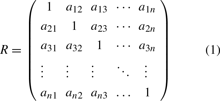
a_ik is the Pearson correlation coefficient between variables y_i and y_k.

Fig. 1

Pearson correlation value of all variables including input and output.

The Pearson correlation coefficient, which exclusively gauges the linear relationship between two variables, ranges from -1.0 to 1.0. When the correlation value between two variables approaches 1, it suggests that one of the two variables can be omitted during the training process of the machine learning model to enhance its performance. The values of the Pearson correlation coefficient between each input variable and the output variable are depicted in the last row of the Pearson correlation matrix (refer to Fig. 1). It’s crucial to note that a correlation coefficient close to or equal to 0 does not necessarily imply independence between two variables. This limitation is inherent to both the Pearson correlation coefficient and linear regression. Consequently, the relationships must be thoroughly assessed using different machine learning techniques such as Shapley Additive Explanations (SHAP) and Partial Dependence Plot (PDP), as discussed in the final section, to accurately quantify these relationships.

It can be observed that certain variables exhibit correlation with each other; for instance, MgO and Al₂O₃ demonstrate a relatively strong correlation of 0.81. However, as these are independent components of tailings essential for studying the influence of chemical composition on the Young modulus of CPB, both variables are retained in the machine learning model construction.

Nevertheless, three variables, namely Gs, D10, and D50, display a very strong correlation close to 1. Therefore, the database will only utilize one of these three variables, specifically D10. In practice, the 13 input variables are categorized into groups based on particle characteristics (Gs, D10, D50, Cu, Cc), chemical composition structure (SiO₂, CaO, Al₂O₃, MgO, and Fe₂O₃), and design conception of CPB (Cement/Tailings, solid content, and curing age). For a comprehensive assessment of the impact of these variable groups on Young modulus values, feature selection via the Pearson correlation matrix is applied. As a result, 11 input variables, comprising particle characteristics (Gs, Cu, Cc), chemical composition structure (SiO2, CaO, Al2O3, MgO, and Fe2O3), and design conception of CPB (Cement/Tailings, solid content, and curing age), are selected for training the machine learning model.

Figure 2 provides details about the distribution of 11 input variables and 1 output variable in the database. In Fig. 2a, it can be seen that most of the data are in the range of D10 content below 0.1% . The Cu data points are evenly distributed across the Cu values, however it can be seen that the data points when the Cu value is greater than 12 have a greater density than the rest (Fig. 2b). The data points of Cc are also concentrated in the range of values below 1.5 presented in Fig. 2c. Figure 2d shows the data distribution of the input variable SiO2 content mainly concentrated in the range of 40-50% . Looking at Fig. 2e, it is easy to see that the data points of this input variable are concentrated towards the side with CaO content less than 20% . Figure 2f shows the richness of the data for Al₂O₃ content, as the data points for this variable are spread evenly across the value scale. MgO content has data points mainly concentrated in the range of 0-5% (Fig. 2g). Similarly, the input variable with data points skewed towards having values less than 5% is observed in Fig. 2h. Figure 2i and 2j show the data distribution of the input variable Cement/Tailings ratio and solid content, respectively. It is easy to see that they have an extremely wide data spectrum with discrete data points spanning the measurement scale. Finally, Fig. 2k presents the curing age data points. Data uses measured intensities at 3, 7, 60 and 17.81 days of age.

Fig. 2

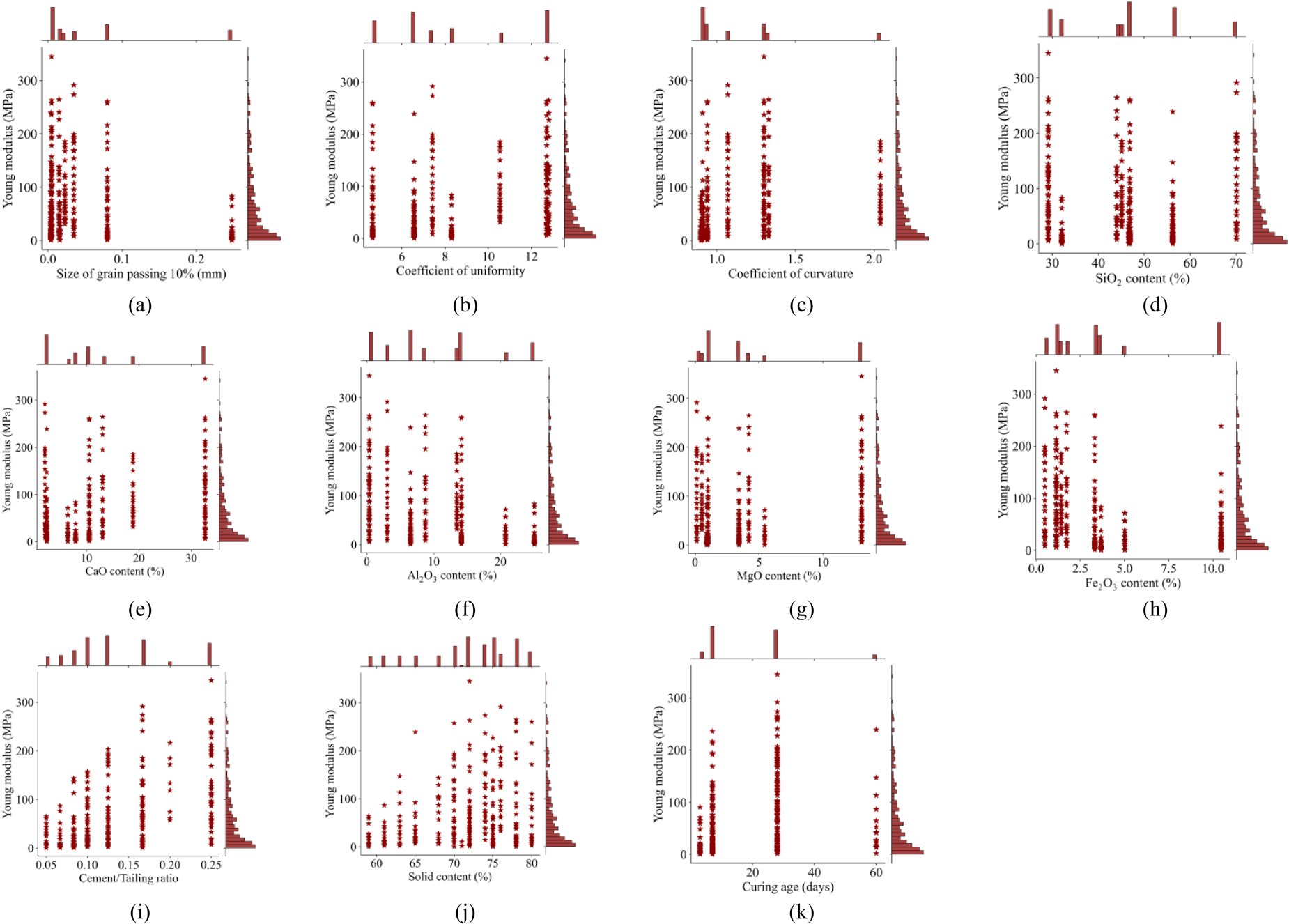
Description of data distribtion between each input and output variables.

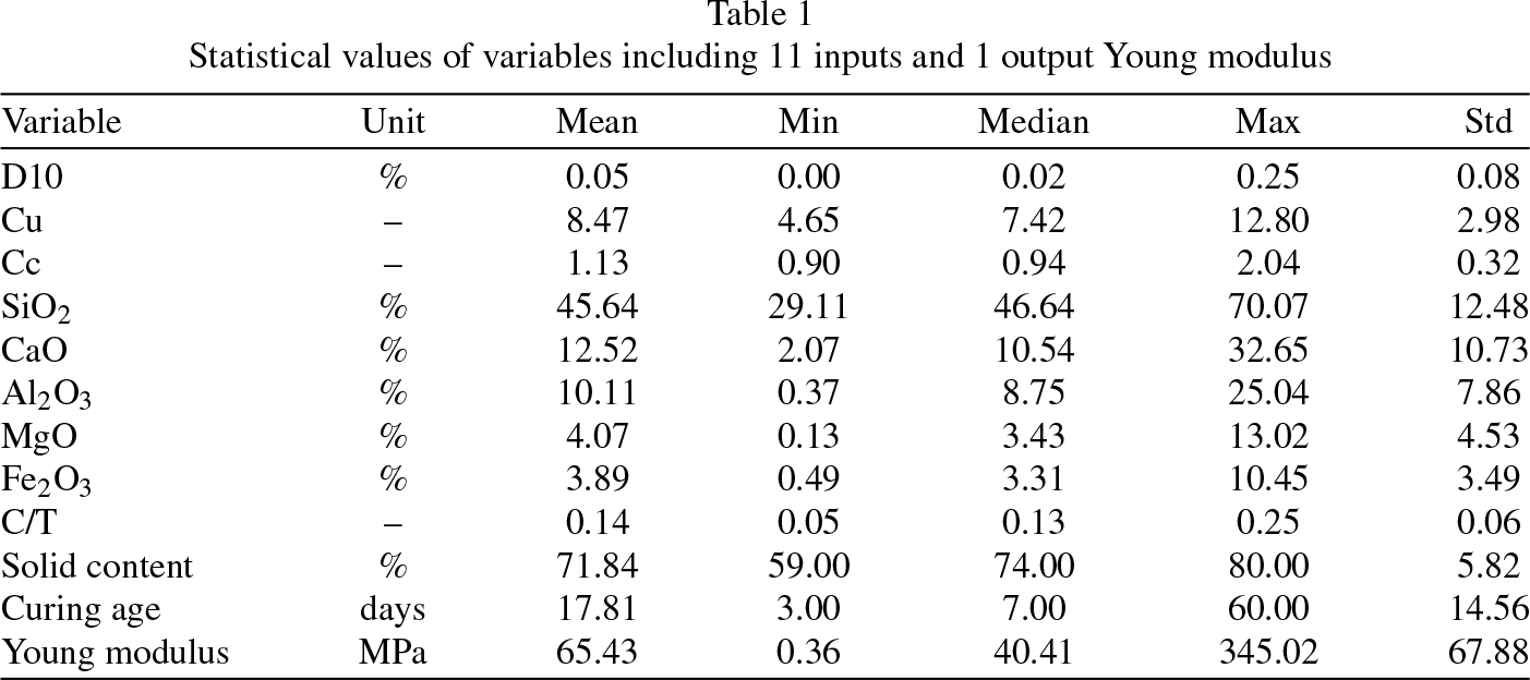
Table 1 shows statistical values of variables including 11 inputs and 1 output Young modulus. The statistical values consisting of minimal, maximal, average and median value, Standard deviation (Std) values of all variables give the applicable range of Machine Learning models.

Table 1

Statistical values of variables including 11 inputs and 1 output Young modulus

Variable	Unit	Mean	Min	Median	Max	Std
D10	%	0.05	0.00	0.02	0.25	0.08
Cu	–	8.47	4.65	7.42	12.80	2.98
Cc	–	1.13	0.90	0.94	2.04	0.32
SiO₂	%	45.64	29.11	46.64	70.07	12.48
CaO	%	12.52	2.07	10.54	32.65	10.73
Al₂O₃	%	10.11	0.37	8.75	25.04	7.86
MgO	%	4.07	0.13	3.43	13.02	4.53
Fe₂O₃	%	3.89	0.49	3.31	10.45	3.49
C/T	–	0.14	0.05	0.13	0.25	0.06
Solid content	%	71.84	59.00	74.00	80.00	5.82
Curing age	days	17.81	3.00	7.00	60.00	14.56
Young modulus	MPa	65.43	0.36	40.41	345.02	67.88

4 Conception of data-driven investigation

4.1 Methodology flowchart of investigation

Figure 3 illustrates the machine learning approach adopted in this study for evaluating the Young modulus of CPB. This approach comprises four main steps:

Fig. 3

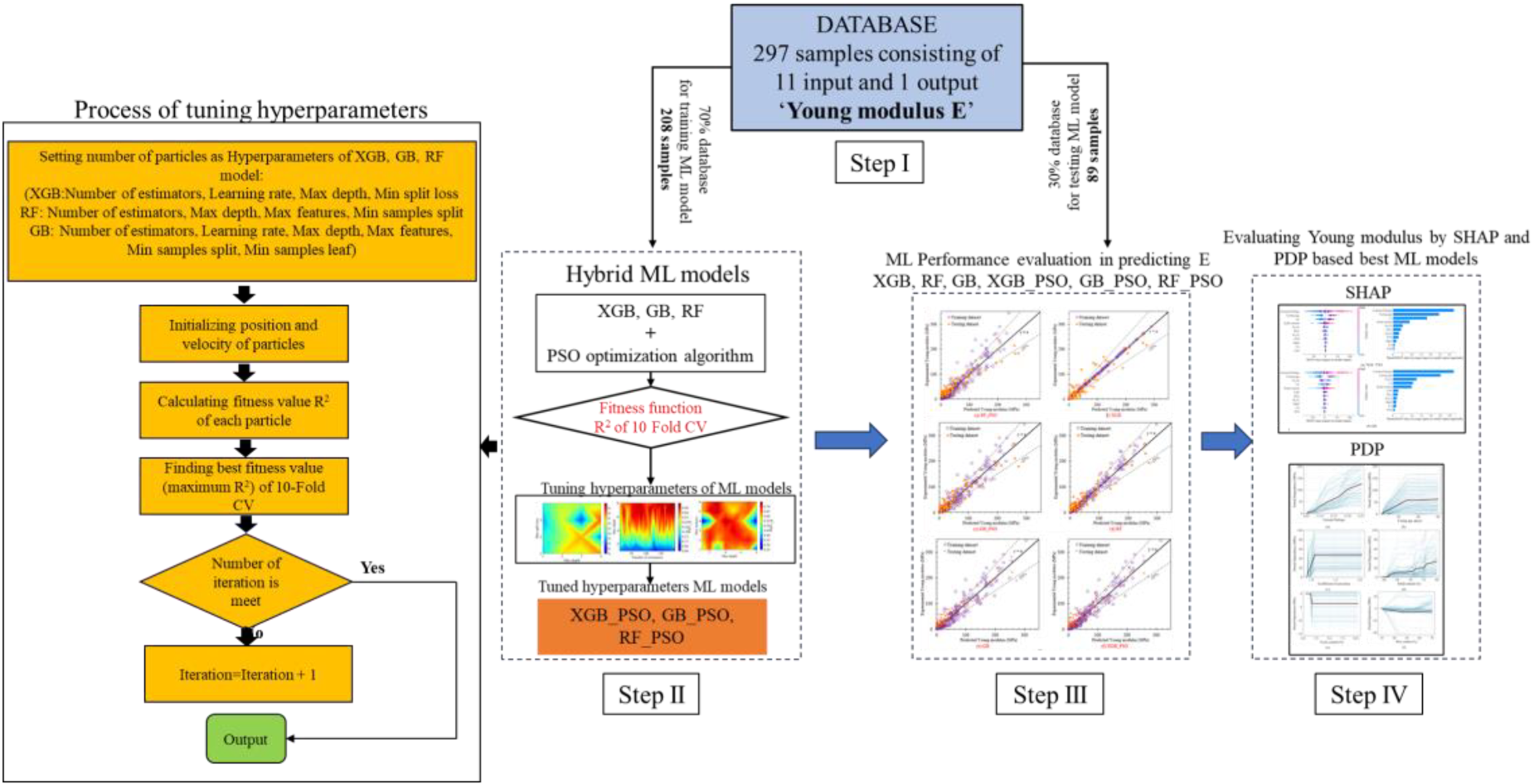
Methodology flowchart of Young modulus investigation using Machine Learning model.

Step I: Feature selection. In this initial phase, the analysis involves the examination of a raw database containing 297 samples and 13 input variables. The number of input variables is reduced from 13 to 11 using the Pearson correlation matrix (refer to Section 2).

Step II: Tuning and Training of 3 hybrid ML models, namely RF-PSO, GB-PSO, and XGB-PSO. During this step, the entire dataset is randomly divided into two segments, with 70% (208 samples) utilized for model training and the remaining 30% for model testing (89 samples). In this process, the raw values of input variables are employed. The accuracy of the tuned hyperparameters of the models is measured using the coefficient of determination (R2).

During this step, the tuning of hyperparameters is carried out with the assistance of metaheuristic algorithms such as Particle Swarm Optimization (PSO) and K-Fold Cross Validation (CV). Drawing inspiration from the studies Shaban et al. [43], and Yan et al. [44], the schematic representation of this process is depicted in Fig. 3. In this procedure, the optimization scores achieved by the metaheuristic models correspond to the R² value of K-Fold CV. At each iteration, the metaheuristic algorithms strive to identify the highest R² value for K-Fold CV. The highest score, R², in the hyperparameter tuning process is determined using K-Fold Cross-Validation with K = 10 iterations to mitigate the risk of overfitting [45]. The optimal hyperparameters will be replacing in 3 shallow ML model RF, GB and XGB for calling RF-PSO, GB-PSO, and XGB-PSO.

Step III: Performance evaluation of 6 ML models. The Young modulus prediction models for CPB are tested using a dedicated dataset. By assessing the prediction performance on this testing dataset, a comparison is made among the six machine learning models. The goal is to identify the two most effective models for predicting the Young modulus of CPB. Subsequently, these two selected models are utilized for interpreting the Young modulus of CPB through the machine learning method in Step IV. The performance evaluation of ML models includes the assessment of three accuracy metrics: coefficient of determination (R²), Root Mean Squared Error (RMSE), and Mean Absolute Error (MAE). These indices are computed as follows:

R^{2} = 1 - [\frac{Σ_{j = 1}^{K} {(y_{j}^{0} - y_{j}^{K})}^{2}}{Σ_{j = 1}^{K} {(y_{j}^{0})}^{2}}]

(3)

RMSE = \sqrt{\frac{1}{K} Σ_{j = 1}^{K} {(y_{j}^{0} - y_{j}^{K})}^{2}}

(4)

MAE = \frac{1}{K} Σ_{j = 1}^{K} | y_{j}^{0} - y_{j}^{K} |

(5)

Step IV: Utilizing interpretability tools, namely Shapley Additive Explanations (SHAP) and Partial Dependence Plot, to elucidate the outcomes of predicting the Young modulus of CPB. Leveraging the two best machine learning models, global interpretation through SHAP values is employed to identify the input variables that most significantly impact the predictability of the machine learning model and exert a substantial influence on the magnitude of the Young modulus of CPB. Simultaneously, the Partil Dependence Plot (PDP 1D) technique is utilized to discern the trend of influence exhibited by the 11 input variables on the development of the Young modulus. Finally, the results of two specific cases of CPB Young modulus testing are explained using local SHAP values.

4.2 Shallow machine learning models with default hyperparameters

In this study, three shallow ML algorithms are used: Extreme Gradient Boosting (XGB) [46], Random Forest (RF) [47], Gradient Boosting (GB) [48] is a powerful algorithm that uses an additive model and a forward subtraction algorithm to realize optimized learning. Random forest (RF) is an optimized version of bagging based on the tree model, creating one tree is definitely not as good as many trees so there is random forest to solve the weak generalization ability of decision trees. The idea of the Extreme Gradient Boosting (XGB) algorithm is to continuously add trees and continuously perform feature decomposition to grow the tree, each time a tree is added, it will actually learn a new function to fit the remainder of the prediction final.

4.3 Hyrid machine learning models with tuned hyperparameters

Hyperparameter optimization involves finding the optimal combination of hyperparameters to maximize the performance of a model. This process entails conducting comprehensive experiments during training, exploring hyperparameters within predefined ranges. Upon completion, the model acquires the most suitable set of hyperparameters for optimal results. Hyperparameters significantly impact the quality control of machine learning models. Adequate regularization hyperparameters can prevent overfitting issues, and adjusting the appropriate number of repetitions can reduce training time. There are two methods for hyperparameter tuning: manual tuning and automatic hyperparameter tuning. Manual tuning grants humans greater control over the process but can be a laborious and time-consuming endeavor, involving extensive testing and resource investment.

Automatic hyperparameter tuning employs metaheuristic algorithms such as Particle Swarm Optimization (PSO). The intricacies of the PSO algorithm are outlined in the investigation conducted by Liu et al. [51]. The PSO algorithm dynamically adjusts particle flying speeds based on individual and collective flight experiences. The formula for the particle swarm algorithm is as follows:

V_{id}^{t + 1} = {wV}_{id}^{t} + c_{1} r_{1} (p_{i}^{d} - x_{i}^{t}) + c_{2} r_{2} (p_{g}^{d} - x_{i}^{t})

(6)

x_{i}^{t + 1} = x_{i}^{t} + V_{id}^{t + 1}

(7)

Here, $x_{i}^{t}$ represents the current location of particle i, $p_{i}^{d}$ is the best-known position of particle i up to this point, and $p_{g}^{d}$ is the best-known position of the entire particle swarm. ‘w’ is a positive constant known as the inertia factor, which linearly decreases with each iteration; ‘c1’ and ‘c2’ are non-negative constants referred to as the cognitive weights and social weights. ‘r1’ and ‘r2’ are random values within the range [0,1], and V_id ∈ [- V_max, V_max] sets the velocity bounds, with ‘Vmax’ as a non-negative constant. The termination criterion for iterations is either reaching the maximum number of iterations or finding the best position of a particle that satisfies adaptive threshold significance. The velocity change in the PSO formula (1) incorporates three components: the inertia factor, cognitive weight, and social weight. These elements collectively determine the performance of PSO and how it maintains balance. Following Blanke’s recommendation [49], the values for ‘w,’ ‘c₁,’ and ‘c₂’ are set to 0.4, 0.7, and 0.7, respectively.

4.4 Shapley additive explanations and partial dependence plot

According to Lunberg et al. [38], SHAP, which stands for Shapley Additive Explanations, was introduced to address challenges related to interpreting complex machine learning models. It draws inspiration from cooperative game theory’s Shapley values and provides a unified framework for explaining the output of any machine learning model. SHAP handles both conditional and interventional distributions by considering the expected value of the model’s output for all possible feature combinations as global interpretation. SHAP ensures additivity by distributing the contribution of each feature to the final prediction in a fair and consistent manner, reflecting the Shapley values. SHAP provides explanations by comparing the model’s output for a specific instance with a baseline reference, highlighting how each feature contributes to the difference in prediction. SHAP calculates the marginal contribution of each feature to the prediction, revealing the impact of individual features while considering their interactions with others. SHAP allows users to understand the impact of each feature on model predictions, enabling informed decisions and actions based on the identified influential factors. SHAP provides a normative evaluation by quantifying the contribution of each feature, allowing users to assess the relative importance of different factors in the model’s predictions. SHAP’s strength lies in its mathematical foundation, rooted in Shapley values, which ensures fair and consistent attribution of contributions to features in a way that respects certain desirable properties, such as additivity and consistency. The framework is versatile and applicable across various machine learning models, making it a widely adopted tool for model interpretation.

SHAP (SHapley Additive exPlanations) addresses the challenge of correlated features by employing cooperative game theory principles, specifically Shapley values. Shapley values allocate the contribution of each feature to the prediction by considering all possible feature combinations. In the context of correlated features, SHAP ensures a fair distribution of influence among the correlated features, preventing biased attributions. This allows SHAP to provide meaningful and reliable explanations even when dealing with interdependencies among features in the dataset.

The Partial Dependency Plot (PDP), a technique we’ll explore first, was developed several decades ago. It showcases the impact that one or two features can have on the predicted outcome of a machine learning model. PDP assists researchers in understanding how model predictions change with variations in different features. The inaugural partial dependence plot was crafted in 2001 by Friedman [35].

5 Results and discussion

5.1 Tuning hyperparameters of machine learning models

Fine-tuning hyperparameters significantly enhances the training and prediction capabilities of the Random Forest (RF), Gradient Boosting (GB), and XGBoost (XGB-PSO) models.

For the RF model, key parameters include max depth, number of estimators (n-estimators), max features, and learning rate [25]. The GB model benefits from fine-tuned parameters influencing individual trees and boosting operations, such as learning rate, number of estimators, max depth, min samples split, max features, and min samples leaf, contributing to model robustness and generalization [25]. The XGB model encompasses tree-specific and learning task-specific hyperparameters, controlling overall behavior and learning processes, including learning rate, number of estimators, max depth, and min split loss [50].

Figure 4 illustrates a heatmap indicating R² value changes for hyperparameter pairs in each hybrid ML model after 1000 iterations. The color transition from green to red signifies the increasing R² values. Notably, after around 500 iterations, the highest R² value stabilizes. Figure 4a displays the fine-tuning results of the XGB-PSO model, showcasing the impact of parameters like max depth, n- estimators, min samples split, and max features. Similarly, Fig. 4b and 4c depict the hyperparameter tuning outcomes for the RF-PSO and GB-PSO models, respectively.

Fig. 4

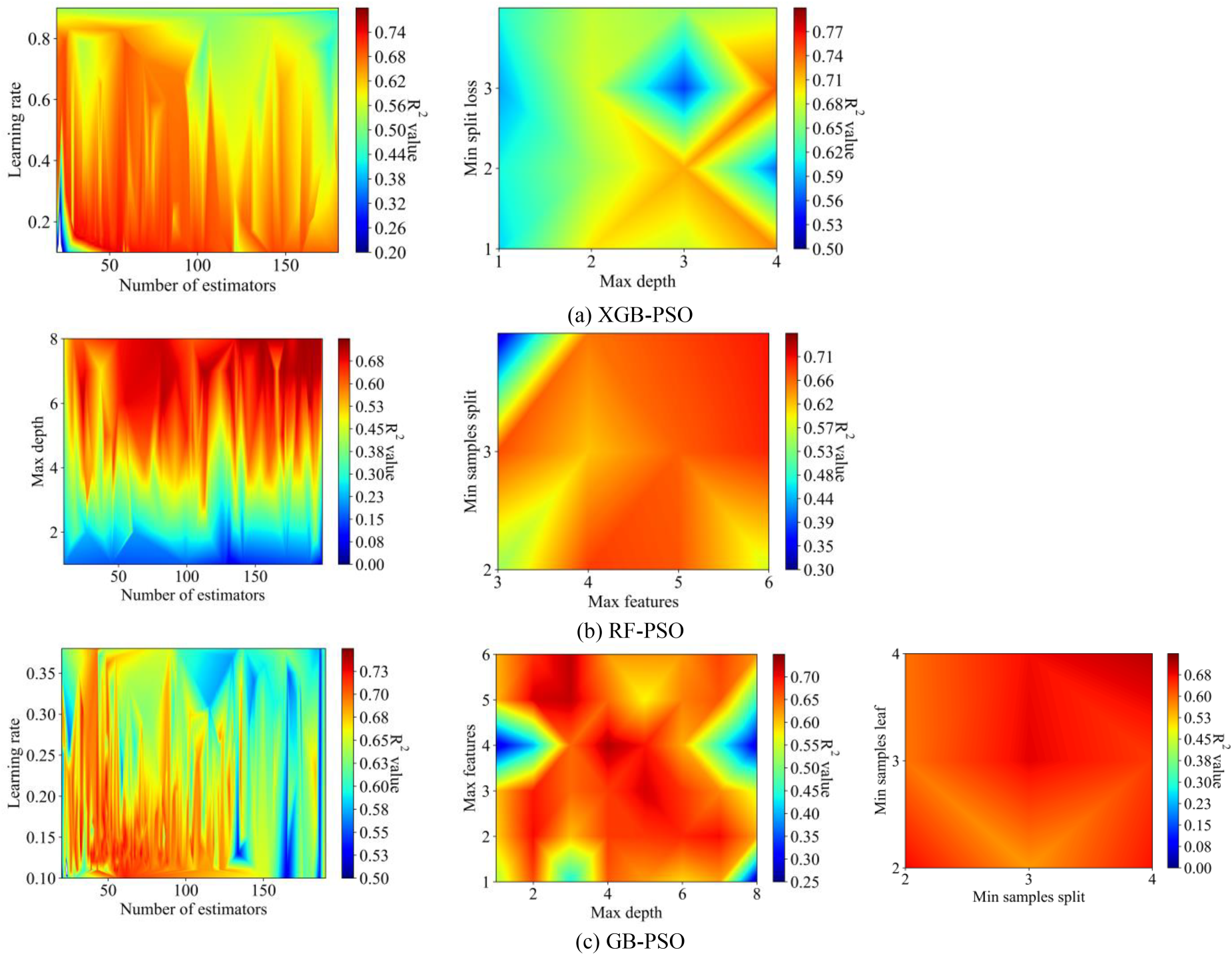
Heatmap of cost optimization R².

In Fig. 4a, increasing the learning rate and n-estimators leads to losses, causing a decrease in R² value. Optimal values are observed when n-estimators is 42 and the learning rate is 0.123. Higher max depth values make the model adept at capturing complex data, and increased min split loss provides smoother results, reaching the best R² when max depth is 4 and min split loss is 2.

Figure 4b reveals the RF-PSO model’s best R² value (0.73) when max depth is 8 and n-estimators is 191. Min samples split and max features also contribute to achieving the highest R², with min samples leaf set at 2.

Figure 4c presents the hyperparameter tuning results for the GB-PSO model, emphasizing the impact of n-estimators, learning rate, max depth, max features, min samples split, and min samples leaf. The optimal configuration is reached with 52 estimators, learning rate of 0.13, max depth of 4, max features of 3, min samples split of 2, and min samples leaf of 3.

5.2 Performance evaluation of ML models in prediction of Young modulus

Young modulus (E) prediction results of models using default hyperparameter: GB, XGB, RF, and hybrid ML models GB-PSO, XGB-PSO, and RF-PSO are presented in Fig. 5 and Table 2 respectively. To evaluate the performance of 6 ML models, use the coefficient of determination (R²), Root Mean Squared Error (RMSE), and Mean absolute error. As proposed by Apostolopoulou et al. [51], the a25-index, a novel engineering metric, is recommended for assessing the accuracy of the ML models, given by a25 = m25/M. Here, M represents the dataset sample size, and m25 is the sample size where the True value/Predicted value falls within the range of 0.75 to 1.25. This index reflects the percentage of samples that align with expected values, exhibiting a variance of no more than 25% from the experimental values.

Fig. 5

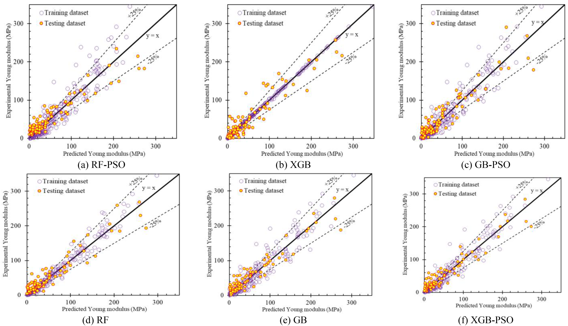
Comparison of predicted Young modulus values and experimental Young modulus values (a) RF-PSO, b) XGB, c) GB-PSO, (d) RF, (e) GB and (f) XGB-PSO model.

Table 2

Summarizing of performance value for 6 ML models

ML model	Training dataset				Testing dataset
	R²	RMSE	MAE	a25 index	R²	RMSE	MAE	a25 index
		(MPa)	(MPa)			(MPa)	(MPa)
RF-PSO	0.866	25.281	16.903	0.498	0.859	23.871	17.401	0.389
XGB	1.000	1.507	0.907	0.966	0.868	23.113	16.545	0.367
GB-PSO	0.891	22.764	15.608	0.507	0.870	22.984	16.216	0.444
RF	0.958	14.101	9.077	0.498	0.891	20.976	15.168	0.389
GB	0.894	22.425	15.438	0.512	0.902	19.886	14.187	0.478
XGB-PSO	0.909	20.783	14.113	0.560	0.906	19.535	13.741	0.467

The prediction results of the RF-PSO model are depicted in Fig. 5a, revealing discrete training data points. This discreteness is evident through evaluation indices: R² = 0.866, RMSE = 25.281 MPa, and MAE = 16.903 MPa. The experimental data points of the RF model also display a substantial degree of dispersion, with the a25 index at approximately 0.389. These obtained indices are considered the lowest among the six models, with R² = 0.859, RMSE = 23.871 MPa, and MAE = 17.401 MPa.

In contrast to the discreteness of the RF-PSO model, the XGB model showcases training data points arranged in an almost perfect linear line (Fig. 5b), as evidenced by the indices: R² = 1.000, RMSE = 1.507 MPa, MAE = 0.907 MPa, and a25 index = 0.966. However, on the test dataset, these indices undergo substantial changes, indicating a potential overfitting issue, with R² = 0.868, RMSE = 23.113 MPa, MAE = 16.545 MPa, and a25 index = 0.367.

Figure 5c presents the distribution of data points for the GB-PSO model, exhibiting discrete distribution. On the test set, this model yields indices of R² = 0.870, RMSE = 22.984 MPa, MAE = 16.216 MPa, and a25 index = 0.444. Next is Fig. 5d, displaying the distribution of data points for the RF model. It is observed that the RF model, with data points within the 25% error range, outperforms the GB-PSO model. This is supported by the indices on the test dataset: R²= 0.891, RMSE = 20.976 MPa, MAE = 15.168 MPa, and a25 index = 0.389.

Figure 5e illustrates the distribution of data points for the GB model, with a considerable number of training set data points within the 25% error range, along with indices of R²= 0.894, RMSE = 22.425 MPa, MAE = 15.438 MPa, and a25 index = 0.512. On the test set, these indices remain relatively stable: R² = 0.902, RMSE = 19.886 MPa, MAE = 14.187 MPa, and a25 index = 0.478.

Finally, Fig. 5f displays the prediction results of the XGB-PSO model. Similar to the GB model, relatively few training data points of the XGB-PSO model fall outside the 25% error range. This is reflected in the indices: R² = 0.909, RMSE = 20.783 MPa, MAE = 14.113 MPa, and a25 index = 0.560. Additionally, the results on the test set are promising: R² = 0.906, RMSE = 19.535 MPa, MAE = 13.741 MPa, and a25 index = 0.467. Compared to the XGB model using default hyperparameters, the XGB-PSO model overcomes overfitting issues and achieves excellent prediction performance. Detailed evaluation indicators for the prediction of Young modulus (E) in MPa are presented in Table 2.

Generally, most research endeavors have predominantly focused on advancing machine learning (ML) methodologies for predicting the Unconfined Compressive Strength (UCS), with limited attention given to ML models predicting the Young’s modulus of Cement Paste Backfill (CPB). Hence, the machine learning model’s performance in predicting the Young modulus in this study is reasonably significant. The predictive accuracy of the Young modulus for the two ML models, GB and XGB-PSO, is found to be 0.902 and 0.906, respectively. These accuracies surpass the previously suggested results by Qi et al. [26] introduced in 2018 with R² = 0.7500.

From these outcomes, it becomes apparent that the shallow ML model, such as the GB model, and the hybrid ML model, XGB-PSO, demonstrate superior predictive performance compared to the other six ML models developed.

5.3 Feature importance analysis for young modulus

To assess the significance of each input variable, the Shapley Additive Explanation (SHAP) is employed for calculating the contribution of each input variable. The SHAP value represents the mean marginal effect of individual variables across all possible combinations of input parameters. The importance of each input variable is derived from its absolute SHAP value, with higher absolute values indicating greater importance. Global feature importance is determined by calculating the absolute SHAP value for all parameters and organizing them in descending order. Illustrated in Fig. 6, the x-axis depicts the SHAP value, while the y-axis presents the feature importance. Points in red (or pink) indicate high feature values corresponding to higher SHAP values. Moreover, Fig. 6 displays a distinct separation between positive and negative SHAP values.

Fig. 6

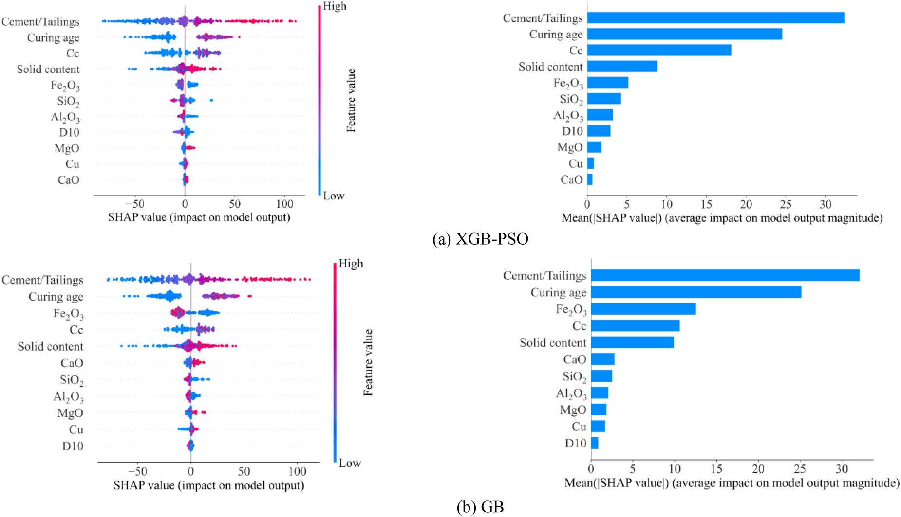
Feature importance analysis using global interpretation SHAP value based two best ML model including XGB-PSO and GB.

The importance of the features of the two models XGB-PSO and GB are determined and ranked in Fig. 6. The graph on the left represents the global SHAP value, each dot represents a sample, and on the right is a histogram representing absolute global SHAP value. Global interpretation SHAP helps extract the features most responsible for the model output. It helps determine the role of a particular feature in the model’s final decision or prediction.

The GB and XGB-PSO models for predicting the Young modulus of CPB were built with 11 input variables. The SHAP plot representing the influence of 11 input variables on the Young modulus (E) prediction in the XGB-PSO model is depicted in Fig. 6a. Among the features, Cement/Tailings exhibits the widest distribution range, spanning long on both sides, signifying its considerable impact as both the smallest and the most significant feature. The solid content feature has a range of values less than 100, with two distinct values distributed at both ends in an increasing direction. While features like MgO, Cu, and CaO have modest sizes, their SHAP values increase with their growth, akin to Cement/Tailings and solid content, contributing to the prediction of E. Curing age and Cc, despite having relatively wide distribution ranges of sample points, exhibit less clear effects on the increase in SHAP values and the prediction of Young modulus E. Features such as Fe₂O₃, SiO₂, Al₂O₃, and D10 exert a negative influence on the SHAP value, indicating that these features reduce the prediction index E. Ranking the features based on the decreasing influence of the XGB-PSO model, we have: Cement/Tailings>Curing age > Cc>solid content > Fe₂O₃ _> SiO₂ _> Al₂O₃ _> D10 > MgO>Cu>CaO.

Similar to the XGB-PSO model, the GB model highlights two features with significant influence on the SHAP value and the Young modulus (E) prediction—Cement/Tailings and Curing age (Fig. 6b). Features such as Fe₂O₃ and Cc exhibit smaller SHAP values than the solid content feature. However, absolute SHAP value in the right, their values surpass that of solid content, indicating that Fe₂O₃ and Cc play a more substantial role in the final prediction. The ranking of feature importance for the GB model is as follows: Cement/Tailings>Curing age > Fe2O3 > Cc>solid content > CaO>SiO2 > Al2O3 > MgO>Cu>D10.

It is evident that the ranking order of the XGB-PSO and GB models is consistent in the two features that exert the greatest influence on the model’s predictions, namely Cement/Tailings and Curing age. Furthermore, another noteworthy result is that, through the global interpretation SHAP values provided by the two models, GB and XGB-PSO, it can be asserted that six input variables are crucial for predicting the Young modulus of CPB using ML models. These input variables include Cement/Tailings, Curing age, Cc, solid content, Fe₂O3 content, and SiO₂ content.

To have a more intuitive view of how a specific feature impacts the prediction results E of the proposed models, the PDP plot has been shown in Fig. 7. Observe Fig. 7a, feature data Cement/Tailings shows an increasing trend in the prediction index E. This can be clearly seen through the feature’s moving average, which is a diagonal line that tends to rise quite steadily. Not increasing slowly like Cement/Tailings, the Curing age increases very quickly, but when it reaches day 27, the value of E increases very little, it is almost impossible to see the increase clearly (Fig. 7b). Similar to the Curing age, Fig. 7c shows that feature Cc has a fairly steep slope, however, after passing 1.1 there is no longer any increase in the predicted value E. Figure 7d shows the increase in the solid content feature is a fairly gentle slope, with content less than 60% the expected value is very small, but then there is an increase. It is noteworthy that when the solid content reached 75%, there was a decrease in the predicted value E but increased again soon after. Observing Fig. 7e, the partial dependence value decreases rapidly until the Fe₂O₃ content reaches about 2%, then stops. The graph showing the partial dependence value when the SiO2 content is below 45% has a clear decrease in this value range, but when the SiO2 content is greater than 60%, the partial dependence value has slightly increased again (Fig. 7f). The two features Al₂O₃ and D10 both show a negative impact on the predicted value E at the first value range and then remain the same as shown in Figs. 7g and 7h respectively. In Fig. 7i, in the range of MgO content below 5%, the influence on the predicted value E is negligible, but after about 5%, this feature shows a rather strong positive influence. The Cu feature has a positive influence on the prediction index E steadily with the increase of the Cu value. Looking at the 7k image, it can be seen that at a value of about 6.5, the increase in the partial dependence value slowed down but soon increased slightly again. Finally, Fig. 7l shows the effect of the CaO feature on the predicted value E. With CaO content below 17%, this feature has almost no effect on the partial dependence value. However, with the increase of CaO content, the partial dependence value has increased to approximately double that of the MgO feature. Through PDP, it can be seen that Cement/Tailings have a very strong positive linear relationship with young modulus. Input variables Cement/Tailings, Vulcanization age, Cc, solids content, Cu and CaO are factors that favor the development of young modulus. The remaining properties Fe₂O₃, SiO₂, Al₂O₃, D10 are factors that have a negative influence on the predicted value of young modulus. However, they only bring negative effects above a certain level and then stabilize.

Fig. 7

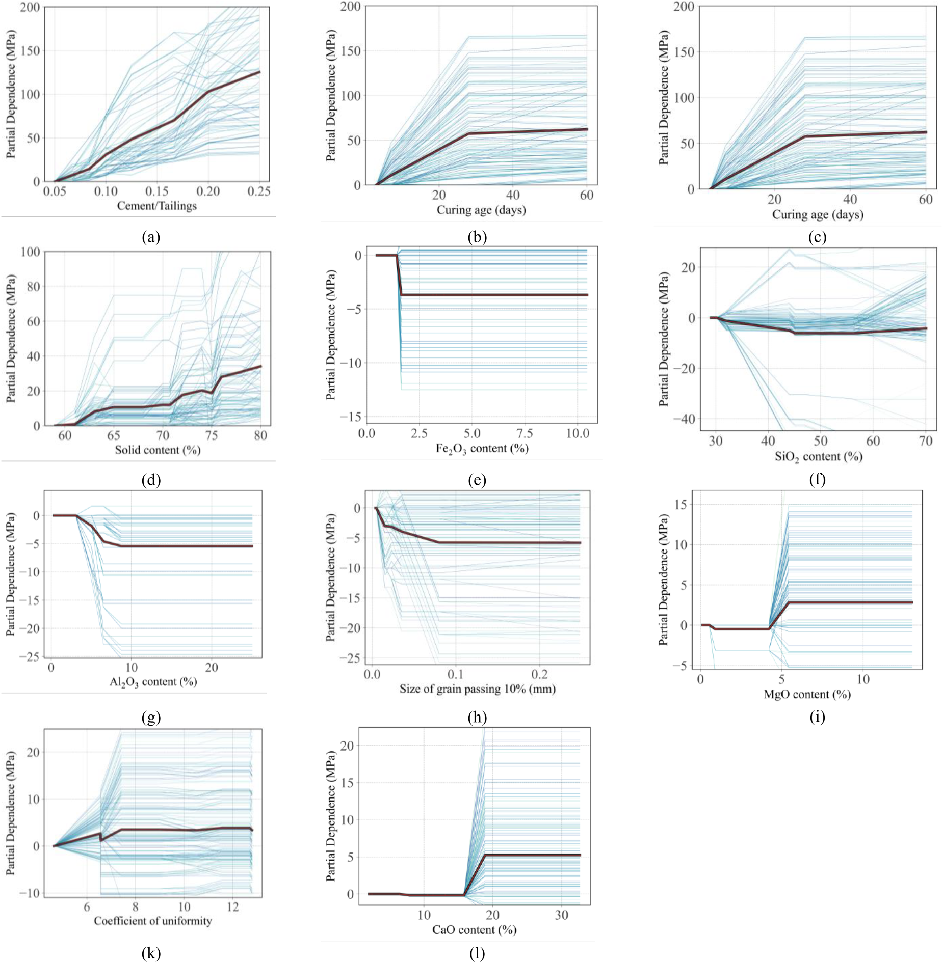
Partial Dependence Plot of 9 input variables on Young modulus.

The outcomes of PDP 1D serve as a valuable resource for the initial investigation of CPB mix designs. Figure 7 facilitates a prompt estimation of Young modulus, allowing for a quick assessment of the gain in shrinkage/swelling associated with individual parameters. By utilizing the initial mix composition, each graph in Fig. 7 provides insights into the Young modulus Gainⁱ attributable to a specific parameter with Predicted = [mean value (65.43) +∑Gainⁱ]. This enables an efficient and effective analysis for the preliminary study of CPB mix designs.

Analyzing the influence of input factors on the Young modulus of CPB involves utilizing Global SHAP values, SHAP value PDP, and SHAP local values. In addition to global interpretations, SHAP also offers valuable insights for explaining model predictions on individual samples. This is achieved through Local SHAP interpretation, where SHAP decomposes the final prediction into a sum of contributions from all the input variables for a specific sample.

Figure 8 illustrates two specific cases with true Young modulus values of 51.19 MPa (Fig. 8a) and 13.47 MPa (Fig. 8b). The XGB-PSO hybrid ML model accurately predicts the Young modulus for each case: 52.35 MPa for case 1 (true value 51.19 MPa) and 13.47 MPa for case 2 (true value 13.47 MPa).

Fig. 8

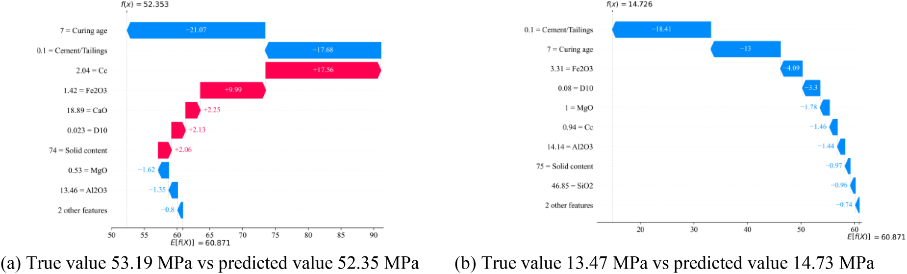
Local interpretation by SHAP value for two specific cases.

SHAP decomposes the final prediction, considering contributions from all input variables relative to a base value of 60.871 MPa, the dataset average. Positive and negative SHAP values indicate features that lead to an increase or decrease in Young modulus, respectively. The length of the bars represents the extent of the impact of each feature on the prediction.

In case 1, with a curing age of 7 days, Cement/Tailings ratio of 0.1, Cc of 2.04, and Fe2O3 content of 1.42%, the primary factors influencing Young modulus, indicated by their SHAP values, are curing age (-21.07 MPa), Cement/Tailings ratio (-17.68 MPa), Cc (+17.56 MPa), and Fe2O3 content (+9.99 MPa). Algebraically adding these SHAP values to the base value results in a predicted Young modulus of 52.35 MPa. For case 2, where Fe₂O₃ content increases to 3.31% and Cc decreases to 0.94 while other input variables remain constant, the SHAP values for Fe2O3 content (-4.09 MPa) and Cc (-1.26 MPa) suggest that increasing Fe₂O₃ content and decreasing Cc lead to a decrease in Young modulus. The predicted Young modulus for case 2 is 14.726 MPa, obtained by algebraically adding these SHAP values to the base value of 60.871. In summary, these specific cases demonstrate that increasing Fe₂O₃ content and decreasing the coefficient of curvature result in a proper decrease in the Young modulus value.

5 Limitations and future work

It is crucial to recognize that the application of the proposed ML model is restricted by the set of parameter values used in both its design and training. Specifically, as indicated in Table 1, the reliability of the ML model is assured for predictions involving 11 input variables within the range of the lowest and maximum values. However, the dependability of the ML model significantly diminishes for input variable values beyond these limits. Despite the satisfactory findings obtained, caution is advised in using the suggested GB and XGB-PSO models. The author emphasizes the need to supplement the existing database with additional experimental data, particularly obtaining higher range values for the 11 input variables and Young modulus, to enhance the overall quality of the database.

The development of the machine learning model solely based on the analysis of the top 5 important input variables, including Cement/Tailings, Curing age, Cc, solid content, Fe₂O₃ content, and SiO₂ content, for predicting the Young modulus of CPB is of utmost significance. The importance of assessing the reliability of prediction results by machine learning models has been emphasized by Shahri et al. [52]. Therefore, future research endeavors should include an evaluation of the reliability of prediction results by machine learning models.

6 Conclusions

This study employed six interpretable machine learning (ML) models, comprising three shallow ML models (XGB, GB, RF) and three hybrid ML models (XGB-PSO, GB-PSO, RF-PSO), to predict the Young modulus of cemented paste backfill (CPB). The shallow models XGB, GB, and RF utilized default parameters, while the hybrid models XGB-PSO, GB-PSO, RF-PSO employed fine-tuned hyperparameters. Evaluation criteria revealed varied performances based on the model, with different outcomes for fine-tuned and default hyperparameters.

The GB shallow ML model and the hybrid ML model XGB-PSO demonstrated superior performance compared to other models. Specifically, on the testing dataset, the GB model achieved impressive results with R² = 0.902, RMSE = 19.886 (MPa), and MAE = 14.187 (MPa). Similarly, the XGB-PSO model exhibited excellent performance, obtaining R²= 0.906, RMSE = 19.535 (MPa), and MAE = 13.741 (MPa).

Beyond achieving highly accurate predictions, the study explored the influence of composition on Young modulus. Input variables such as Cement/Tailings, Curing age, Cc, solids content, Cu, and CaO positively impacted Young modulus development. Conversely, properties like Fe₂O₃, SiO₂, Al₂O₃, D10 exerted a negative influence, albeit limited to a certain level. Notably, global interpretation using SHAP values from the GB and XGB-PSO models identified six crucial input variables for predicting Young modulus: Cement/Tailings, Curing age, Cc, solid content, Fe₂O₃ content, and SiO₂ content. PDP analysis proved effective for the preliminary study of CPB mix designs.

Footnotes

Acknowledgments

This research is funded by University of Transport Technology (UTT) under grant number -DTT-D2022-17.

Conflict of interest

The authors declare that there is no conflict of interest.

Availability of data and material

Data will be made available on request.

References

Liu

D.L.

Wang

K.F.

Yang

Q.H.

, Heavy metal accumulation characteristics of 3 pioneer plants in wasteland of coalmine tailing in mingshan, Applied Mechanics and Materials246–247 (2013), 566–570.

Muñoz

M.A.

Guzman

J.G.

Zornoza

Moreno

Faz

Lal

, Effects of biochar and marble mud on mine waste properties toreclaim tailing ponds,, Land Degradation & Development27 (2016), 1227–1235.

Yilmaz

, Advances in reducing large volumes of environmentally harmful mine waste rocks and tailings, Gospodarka Surowcami Mineralnymi T. 27z. 2 (2011), 89–112.

Menchaca-Ballinas

L.E.

Escalante-García

J.I.

, Limestone asaggregate and precursor in binders of waste glass activated by CaOand NaOH, Construction and Building Materials262 (2020), 120013.

Saedi

Jamshidi-Zanjani

Darban

A.K.

, A review of additives used in the cemented paste tailings: Environmental aspects and application, Journal of Environmental Management289 (2021), 112501.

Fall

, Effect of tailings properties on paste backfill performance, (n.d.).

Libos

I.L.S.

Cui

, Effects of curing time, cement content, and saturation state on mode-I fracture toughness of cemented paste backfill, Engineering Fracture Mechanics235 (2020), 107174.

Chen

Wang

Liu

Yao

Mitri

H.S.

, Influence of binder types and temperatures on the mechanical properties and microstructure of cemented paste backfill, Advances in Civil Engineering2021 (2021), e6652176

Yang

Wang

Arlin Bruno

Zhou

Wang

, Effect of mixing time on hydration kinetics and mechanical property of cemented paste backfill, Construction and Building Materials247 (2020), 118516.

10.

Fall

Benzaazoua

Saa

E.G.

, Mix proportioning of underground cemented tailings backfill, Tunnelling and Underground Space Technology23 (2008), 80–90.

11.

Vergne

, Rules of thumb for the hard rock mining industry, Hard Rock Miner’s Handbook (2000).

12.

Zhang

, Experimental investigation on mechanical properties of in situ cemented paste backfill containing coal gangue and fly ash, Advances in Civil Engineering2020 (2020), e7964267.

13.

Standard test method for compressive strength of cylindrical concrete specimens (2001).

14.

Najafzadeh

Basirian

, Evaluation of river water quality index using remote sensing and artificial intelligence models, Remote Sensing15 (2023), 2359.

15.

Najafzadeh

Basirian

, Vulnerability of the rip current phenomenon in marine environments using machine learning models, Results in Engineering21 (2024), 101704.

16.

Tran

V.Q.

, Using artificial intelligence approach for investigating and predicting yield stress of cemented paste backfill, Sustainability15 (2023), 2892.

17.

Xiao

Wang

Chen

Bin

Wang

Wei

, Strength investigation of the silt-based cemented paste backfill using lab experiments and deep neural network, Advances in Materials Science and Engineering2020 (2020), 1–12.

18.

Orejarena

Fall

, Artificial neural network based modeling of the coupled effect of sulphate and temperature on the strength of cemented paste backfill, Can. J. Civ. Eng.38 (2011), 100–109.

19.

Fourie

Chen

Zhang

, A strength prediction model using artificial intelligence for recycling waste tailings as cemented paste backfill, Journal of Cleaner Production183 (2018), 566–578.

20.

Fourie

Chen

, Neural network and particle swarm optimization for predicting the unconfined compressive strength of cemented paste backfill, Construction and Building Materials159 (2018), 473–478.

21.

Zhang

Han

, Strength prediction and application of cemented paste backfill based on machine learning and strength correction, Heliyon8 (2022), e10338.

22.

Chen

Fourie

Zhang

, An intelligent modelling framework for mechanical properties of cemented paste backfill, Minerals Engineering123 (2018), 16–27.

23.

Zhou

Shi

Jahed Armaghani

Chen

Huang

, Developing a hybrid model of salp swarm algorithm-based support vector machine to predict the strength of fiber-reinforced cemented paste backfill, Engineering with Computers37 (2021), 3519–3540.

24.

Ngo

Q.T.

Ngo

C.T.

Nguyen

Q.H.

Nguyen

H.N.

Nguyen

L.Q.

Nguyen

K.Q.

Tran

V.Q.

, Data-driven approach in investigating and predicting unconfined compressive strength of cemented paste backfill, Materials Today Communications37 (2023), 107065.

25.

Pedregosa

Varoquaux

Gramfort

Michel

Thirion

Grisel

Blondel

Prettenhofer

Weiss

Dubourg

Vanderplas

Passos

Cournapeau

Brucher

Perrot

Duchesnay

, Scikit-learn: Machine Learning in Python, Journal of Machine Learning Research12 (2011), 2825–2830.

26.

Tran

V.Q.

, Hybrid gradient boosting with meta-heuristic algorithms prediction of unconfined compressive strength of stabilized soil based on initial soil properties, mix design and effective compaction, Journal of Cleaner Production (2022) 131683.

27.

Wolpert

D.H.

Macready

W.G.

, No free lunch theorems for optimization, IEEE Transactions on Evolutionary Computation1 (1997), 67–82.

28.

Nguyen

X.H.

Phan

Q.M.

Nguyen

N.T.

Tran

V.Q.

, Tran, Interpretable machine learning model for evaluating mechanical properties of concrete made with recycled concrete aggregate, Structural Concrete n/a (n.d.).

29.

Quan

, Tran, Machine learning approach for investigating chloride diffusion coefficient of concrete containing supplementary cementitious materials, Construction and Building Materials328 (2022), 127103.

30.

Kennedy

Eberhart

, Particle swarm optimization, in: Proceedings of ICNN’95 –International Conference on Neural Networks4 (1995), 1942–1948.

31.

Cheng

Y.M.

Chi

Wei

W.B.

, Particle swarm optimization algorithm for the location of the critical non-circular failure surface in two-dimensional slope stability analysis, Computers and Geotechnics34 (2007), 92–103.

32.

Linardatos

Papastefanopoulos

Kotsiantis

, Explainable AI: A review of machine learning interpretability methods, Entropy23 (2021), 18.

33.

Rudin

, Stop explaining black box machine learning models for high stakes decisions and use interpretable models instead, Nat Mach Intell1 (2019), 206–215.

34.

Barredo Arrieta

Díaz-Rodríguez

Del Ser

Bennetot

Tabik

Barbado

Garcia

Gil-Lopez

Molina

Benjamins

Chatila

Herrera

, Explainable ArtificialIntelligence (XAI): Concepts, taxonomies, opportunities andchallenges toward responsible AI,, Information Fusion58 (2020), 82–115.

35.

Molnar

, Interpretable Machine Learning: A Guide For Making Black Box Models Explainable, Independently Published, 2022.

36.

Ali

Abuhmed

El-Sappagh

Muhammad

Alonso-MoralR.

J.M.

Confalonieri

Guidotti

Del Ser

Díaz-Rodríguez

Herrera

, Explainable ArtificialIntelligence (XAI): What we know and what is left to Trustworthy Artificial Intelligence,, Information Fusion99 (2023), 101805.

37.

Ribeiro

M.T.

Singh

Guestrin

, “Why Should ITrust You?”: Explaining the Predictions of Any Classifier (2016).

38.

Lundberg

S.M.

Erion

Chen

DeGrave

Prutkin

J.M.

Nair

Katz

Himmelfarb

Bansal

Lee

S.-I.

, From local explanations to global understanding with explainable AI for trees, Nat Mach Intell2 (2020), 56–67.

39.

Linardatos

Papastefanopoulos

Kotsiantis

, Explainable AI: A review of machine learning interpretability methods, Entropy23 (2021), 18.

40.

Brady

B.H.G.

Brown

, Rock Mechanics For Underground Mining, Chapman and Hall1993 (2006).

41.

Naik

D.L.

Kiran

, A novel sensitivity-based method for feature selection, Journal of Big Data8 (2021).

42.

Zhang

, A novel feature selection method based on global sensitivity analysis with application in machine learning-based prediction model, Applied Soft Computing85 (2019), 105859.

43.

Shaban

W.M.

Yang

Elbaz

Xie

, Fuzzy-metaheuristic ensembles for predicting the compressive strength of brick aggregate concrete, Resources, Conservation and Recycling169 (2021), 105443.

44.

Yan

Shen

S.-L.

Zhou

Chen

, Prediction of geological characteristics from shield operational parameters by integrating grid search and K-fold cross validation into stacking classification algorithm, Journal of Rock Mechanics and Geotechnical Engineering14 (2022), 1292–1303.

45.

Brownlee

, Machine Learning Mastery with Python: Understand Your Data, Create Accurate Models and Work Projects End-to-end, 2016.

46.

Chen

Guestrin

, XGBoost: A Scalable Tree Boosting System, Proceedings of the 22nd ACM SIGKDD International Conference on Knowledge Discovery and Data Mining (2016) 785–794.

47.

Breiman , Random forests, MACH LEARN 200145(1) (2001), 5–32.

48.

Friedman

, Greedy Function Approximation: A Gradient Boosting Machine, Annals of Statistics29 (2001), 1189–1232.

49.

Simon Blanke , Hyperactive: An optimization and data collection toolbox for convenient and fast prototyping of computationally expensive models (2019).

50.

Brownlee

, XGBoost With Python: Gradient Boosted Trees with XGBoost and scikit-learn, Machine Learning Mastery 2016.

51.

Apostolopoulou

Asteris

P.G.

Armaghani

D.J.

Douvika

M.G.

Lourenço

P.B.

Cavaleri

Bakolas

Moropoulou

, Mapping and holistic design of natural hydraulic lime mortars, Cement and Concrete Research136 (2020) 1061

52.

Abbaszadeh Shahri

Shan

Larsson

, A novel approach to uncertainty quantification in groundwater table modeling by automated predictive deep learning, {Nat Resour Res31 (2022), 1351–1373.