Non-stationary signal analysis utilizing VMD and EMD algorithm for multiple fault classification for industrial applications

Abstract

The Hilbert spectrum images of intrinsic mode functions (IMF) of empirical mode decomposition (EMD) analysis and variational mode decomposition (VMD) analysis of faulty machine vibration signals are used in deep convolutional neural network (DCNN) for machine fault classification in which the DCNN automatically learns the features from spectral images using convolution layer. Though both EMD and VMD analysis suit well for non-stationary signal analysis, VMD has the merit of aliasing free IMFs. In this paper, the performance improvement of DCNN classification for a non-stationary vibration signal dataset using VMD is brought out. The numerical experiment uses the Hilbert spectrum images of 4 EMD-IMFs and 4 VMD-IMFs in DCNN to classify 10 different faults of the Case Western Reserve University (CWRU) bearing dataset. The confusion matrices are obtained and the plot of model accuracies in terms of epochs for the DCNN is analysed. It is shown that the spectrum images of one of the four EMD-IMFs, IMF₀, give a validation accuracy of 100% and in the case of VMD the spectrum images of two of the four VMD-IMFs, IMF₀, and IMF₁ give a validation accuracy of 100%. This reveals that non-aliasing IMFs of VMD are better at classifying bearing faults. Further to bring out the merits of VMD analysis for non-stationary signals the numerical experiment is conducted using VMD analysis for binary fault classification of the milling dataset which is more non-stationary than the bearing dataset which is proved by plotting the statistical parameters of both datasets against time. It is found that the DCNN classification is 100% accurate for IMF₃ of VMD analysis which is much better than the 81% accuracy provided by EMD analysis as per existing literature. The performance comparison highlights the merits of VMD analysis over EMD analysis and other state-of-the-art methods and ensemble learning methods.

Keywords

Deep convolution neural network empirical mode decomposition hilbert transform intrinsic mode function variational mode decomposition ensemble learning

List of abbreviations

Abbreviation

Description

IMF

greaterthan Intrinsic Mode Functions

EMD

greaterthan Empirical Mode Decomposition

VMD

greaterthan Variational Mode Decomposition

DCNN

greaterthan Deep Convolutional Neural Network

greaterthan Hilbert Transform

greaterthan Ensemble Learning

greaterthan Machine learning

greaterthan Inner Race (fault name)

greaterthan Ball (fault name)

greaterthan Orthogonal (fault name)

greaterthan Drive End (data)

CWRU

greaterthan Case Western Reserve University

ReLU

greaterthan Rectified Linear Units

1 Introduction

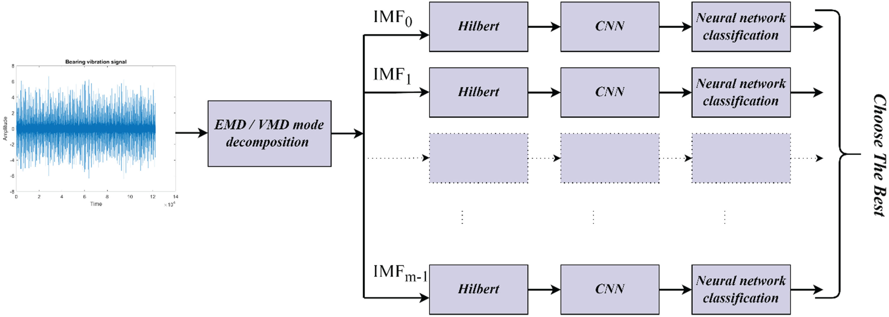
The process of detecting machine faults advanced in time is called predictive maintenance [31] and vibration analysis is a successful tool to execute condition monitoring for industrial equipment to identify and predict failure. This is highly useful for fault diagnosis and equipment management for rotating machines which usually generate vibration signals [11]. Almost all vibration measuring devices perform Fast Fourier Transform (FFT) for signal analysis [4]. In recent days, machine learning (ML) methods [1] have become popular for the extraction of fault information from the vibration signals and help in fault classification. The fault investigation using ML follows two steps: extraction of features from the vibration signals and learning the model from the features [23]. The most common vibration signal features used are mean, root mean square, skewness, maximum, minimum, standard deviation, range, kurtosis, standard deviation, variation, root mean square (RMS), absolute maximum, skewness, kurtosis, crest factor, margin factor, shape factor, impulse factor, A factor of variance, [12] B factor of variance, etc. These features have been used in many ML algorithms like support vector machine (SVM), k-nearest neighbor (KNN), Kernel Bayes, [28] Multilayer perceptron, Decision trees, sparrow search algorithm (SSA) [7], etc to forecast machine faults. A deep convolution neural network (DCNN) is a robust ML approach for image classification and segmentation [5, 16]. In recent days, the method of representing vibration signals in form of images and learning the DCNN model is gaining a lot of attention as DCNN does not require a separate feature extraction stage and automatically learns the features. A recent study [25] uses a convolutional neural network (CNN) to achieve an accuracy of over 96% by reshaping the one-dimensional CWRU vibration data into time-domain images of two dimensions. In another study [27], an accuracy of 98% is attained using a similar technique of altered time-domain images and Alexa-net-based transfer learning architecture [47]. As frequency-domain analysis reveals many of the signal’s hidden specifics, it performs more accurately than time-domain analysis. In a different study [27], a classification efficiency of 99% is shown using frequency-domain sub-spectrograms of vibration signals as images in a CNN transfer learning architecture based on Alexa-net. The main advantage of both approaches [27, 47] is that they both employ transfer learning architecture, which is characterized by very high accuracy and builds on the prior learning completed in Alexa-net. Continuous wavelet transform (CWT) is used in another study [53] to obtain signal spectra, and employing them in CNN, a very high accuracy of 99% is shown. Many researchers are interested in using the intrinsic mode function (IMF) derived by empirical mode decomposition (EMD) of vibration signals for additional analysis [10, 13, 51]. This fits significantly better for non-stationary signals and the typical process followed generally in ML techniques for vibration analysis for fault classification is shown in Fig. 1. However, on a SVM-based classifier, the CNN learned features and other time-domain features of IMF signals are used, and an accuracy of 99% is shown [51]. In EMD entropy features Stacked sparse denoising autoencoder (SSDAE) approach a precision of 99.55% is achieved [10].

Fig. 1

Basic machine learning framework of vibrational analysis.

In our previous published work, [32] the spectral images of empirical mode decomposition-intrinsic mode function (EMD-IMF) signals obtained using short-time Fourier transform (STFT) are trained using DCNN, and it is shown that for fault classification, the method gives a better classification accuracy than that of using spectral images of original signals. Using DCNN eliminates the need for a separate feature extraction stage as it learns features automatically from the training images. The numerical experiment is conducted using the bearing dataset for the fault classification problem and it is found that both methods gave a result of 100% validation accuracy for certain IMFs. As an ablation study, to bring out the efficacy of the EMD method, the numerical method is conducted for both methods on a simple binary classification problem using a milling dataset which is more nonstationary in nature. The result shows that the EMD-IMF method is better than the method that uses the spectrum of the original signal. For this milling dataset which is non-stationary in nature, the validation accuracy of the DCNN model when using a spectrum of original signals is 40% and that of the EMD-IMF method is 81% validation accuracy. This brings out the performance improvement of the method using EMD for non-stationary scenarios. Variational mode decomposition (VMD) is another method that is much more suitable for non-stationary signals and as variational mode decomposition-intrinsic mode function (VMD-IMF) are band-limited and alias-free the spectrum images obtained will lead to better results over EMD-IMFs. Considering the merits of VMD, this paper proposed to use spectrum images of VMD-IMF signals of bearing data and milling data in DCNN to demonstrate a better accuracy than the EMD-IMF method.

This paper aims to represent the Hilbert transform of IMF obtained using VMD spectral images to be trained with DCNN. The typical methodology is given in Fig. 1 and the proposed method is illustrated in Fig. 2 which differs from the way the IMFs are used. It can be observed that in the method given in Fig. 1, the entropies of the IMFs are used as an additional feature, and in the proposed method the complete IMF variations in the form of Hilbert spectrum are utilized in DCNN to learn the useful features. From Fig. 2 it can be observed that multiple CNN training is involved which is similar to classical ensemble learning (EL) in which a strong classifier is built by combining weaker classifiers.

Fig. 2

The proposed machine learning framework of vibrational analysis.

In this paper numerical experiment is conducted for both bearing and milling datasets using both EMD-IMF and VMD-IMF. Four IMF signals obtained by EMD and VMD are used and it is found that the proposed VMD method classifies 10 different fault classes of the CWRU-bearing dataset with validation accuracy of 100% at certain IMFs. It is also inferred that most of the VMD-IMFs perform better than EMD-IMFs. For milling data, the proposed VMD-IMF method gives a validation accuracy of 100% which is much better than the accuracy of the EMD method which is 81%. Hence this work brings out the efficacy of using full EMD/VMD-IMF information of vibration signals in DCNN in classifying the machine faults and also demonstrates the merits of VMD over EMD. The other key inference made is based on how this approach is different from the EL method. Though this method involves multiple CNN training it ends with one best strongest model with 100% accuracy and thus it is required to deploy only one strongest model finally that reduces computation cost. The research contribution in this paper can be summarized as follows. –

Demonstration of using Hilbert spectrogram images of IMF of EMD/VMD in DCNN learning instead of a conventional parametric approach for CWRU bearing dataset.

–

The merits of aliasing free VMD-IMF over EMD-IMF are brought out by showing that two VMD-IMFs IMF₀ and IMF₁ result in 100% validation accuracy for CWRU bearing dataset.

–

An ablation study to bring out the robustness of the VMD approach, by applying to the milling dataset which is more non-stationary than the bearing dataset. The result obtained is 100% validation accuracy for VMD-IMF₃ which is better than the EMD method.

–

The merits of the proposed VMD approach over the EL approach are studied and reported.

2 Related work

There are so many research works that have been carried out in the area of automatic machine fault classification using vibration analysis and, in this section, some of the important related works are discussed in detail. In Section 1, the evolution of fault classification methods using vibration analysis starting from FFT analysis to the ML method is discussed. The discussion is also made on various important useful parameters for vibration analysis. The merits of using image representation of vibration signal in DCNN are also discussed in the same section. The novelty of our proposed work is to use Hilbert spectral images of IMFs obtained by EMD/VMD for very high performance in terms of validation accuracy. In this section, the research works that brought out the significance of EMD and VMD in machine fault classification problems are discussed. The modalities of using IMFs of EMD and VMD in the ML algorithm are also highlighted in this section. The other key discussion that is made in this section is on related works that are done based on EL.

The signal decomposition method increases the diagnostic efficiency of rotating machinery by reducing signal complexity. The well-known decomposition technique EMD, created by Huang et al., has been utilized for decades to detect numerous rotating equipment issues [20, 22, 41, 54]. EMD is a time-frequency analysis method and is demonstrated in signal processing methods in many previous literatures. Instead of relying on preset parameters, the EMD analysis takes into account the signals’ local time scales [19]. In comparison to typical methods like discrete wavelet analysis, the enhanced EMD approach exhibits adaptability, orthogonality, and robustness. In EMD the input signal is broken down into a collection of IMFs and every IMF can be seen as the signal’s fundamental function. The EMD technique may perform better than conventional techniques when the vibration signals are nonlinear and nonstationary. Furthermore, EMD is a self-adjusting processing technique. EMD adapt to the sample rate and noise [49]. In a recent work, a combined approach known as bi-spectrum based EMD (BSEMD) [37] is illustrated to identify machine faults. In a different work, Fuzzy C-means (FCM) clustering of vibration images acquired by empirical mode decomposition-pesudo-Wigner-Ville distribution (EMD-PWVD) is demonstrated [14] in which EMD-PWVD converts vibration data with varying fault degrees into contour time-frequency images then the energy distribution values of the vibration images are utilized as an image feature and the images are segmented to determine the machine faults. Later on, several techniques for improving EMD have been developed, including ensemble empirical mode decomposition (EEMD). VMD, a new signal decomposition technique that may diagnose rotating equipment more accurately than both EMD and EEMD methods is studied [29, 57, 58]. Integrating EMD/VMD analysis in ML is tricky and challenging. One of such integration done in a use case is illustrated in Fig. 2 in which entropies of IMFs are used as additional parameters along with other features learned from STFT using CNN [51] and the accuracy shown is about 99.75% for CWRU bearing dataset [42]. Some work demonstrated the usage of EMD/VMD analysis signals directly in CNN for better accuracy. The One- dimensional (1D) vibration signal is subjected to EMD analysis to get a multi-dimensional IMF matrix which is used directly in CNN and an accuracy of 99.79% is achieved using CWRU bearing dataset. In another work in place of EMD analysis, VMD analysis is proposed for improved accuracy [30]. One-dimensional convolution neural network (1D-CNN) based ML architecture is also studied for machine fault classification using EMD-IMFs [34]. In a very recent paper EMD based multi-scale CNN is proposed to improve the accuracy of fault classification up to 99.86% [34]. As already discussed, VMD analysis is aliasing free and more suitable for fault classification and this is demonstrated in several works [8, 50, 59].

In this section, another class of ML method considered for discussion is EL in which [9, 26, 35, 38– 40, 52, 55] a global decision is taken from the outputs of several independent classifiers to get very high accuracy. One of the popular vastly used EL method is random forest algorithm [6, 43] in which multiple ML models are used in parallel and the result is evaluated using a voting scheme. EL is applied in many works related to machine fault classification using vibration analysis [15, 24, 38, 44, 60] In this discussion focus is given to CNN based EL. A CNN based EL is proposed in which multiple classifiers with different activation functions are used and the final classification result is obtained [38] for CWRU bearing dataset. The proposed method shows a result of 100%, 89.33%, 100%, 98.04%, 98.04%, 100%, 95.29%, 100%, 90.91%, 73.02%, 85.22%, 99.01% for various faults. The result is found to be superior than that of SVM and boosting method. A similar multiple CNN classifiers and EL algorithm is implemented to show that the EL algorithm evaluates the results accurately by combining the individual results of the CNN classifiers with accuracy ranges like 0.9833, 0.9783, 0.9627, 0.9410, 0.9802, 0.9470, 0.9659, 0.9800, 0.9745, 0.9390 [55] using CWRU bearing dataset. In a recent work, imbalanced ensemble method with DenseNet and Evidential Reasoning rule (IEMD-ER) is proposed for the Paderborn University bearing dataset and proved to be superior among other EL. It should be noted that EL involves multiple learning models and multiple deployments [46] of the individual classifiers that demands more computation power.

3 Proposed work

As we discussed in Section 2 there are several ways to incorporate learning of IMF of EMD/VMD signals and in this work, it is proposed to use the Hilbert spectrum images of IMF signals along with DCNN as a novel approach. It is proposed to bring out the merits of using spectrum images of IMF-VMD of vibration signal over IMF-EMD of vibration signals in DCNN to classify the machine faults in DCNN. The study is done using two different datasets

1.
Bearing dataset CWRU (10 different machine faults) [62].
2.
Milling dataset NASA (highly non-stationary and 2 different simulated machine faults) [63].

The performance of DCNN learning on EMD spectrum images is already well proven to be very high close to 100% validation accuracy for the first dataset [32]. As an ablation study, to bring out the fact that EMD spectrum learning is better with DCNN, dataset 2 is used in which more non-stationary process are involved and this will be explained in Subsequent section 3.4. To create the spectrum images Hilbert transform is used. In this section, the methodology of spectrum image creation and the dataset description are discussed in detail. The nonstationary nature of the milling dataset is also illustrated in this section.
3.1 Methodology for creating Hilbert spectral images

From the dataset, the vibration signals for healthy and unhealthy situations are extracted, and then separated into K-short, overlapping signals that overlap for T time units. In this work, we took into account two datasets [62, 63] and the K depends on the dataset we choose. Each of these K signals is regarded as a member of a fault class. For each of these signals, EMD is applied to get R intrinsic mode functions (IMF). Hilbert transform is applied to these mode functions with a window length of N and 50% overlapping to get spectrum images as shown in Fig. 3. A similar procedure is repeated to get the spectrum images by applying VMD in place of EMD shown in Fig. 4. The IMF obtained using both EMD and VMD will distribute every bit of information about the time-domain signal. The IMF is still the time-domain function that acts as the signal’s roughly parallel structure [2].

Fig. 3

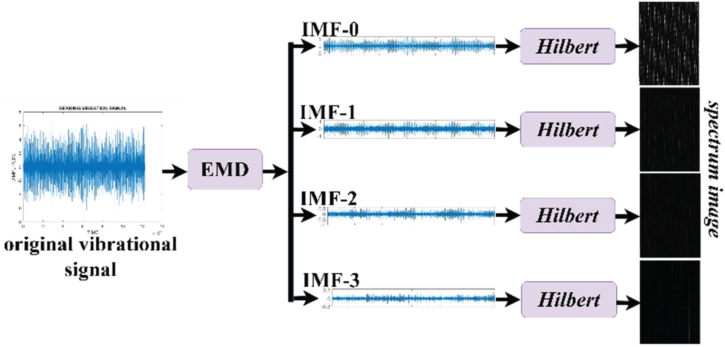
Hilbert spectrum creation of EMD-IMFs.

Fig. 4

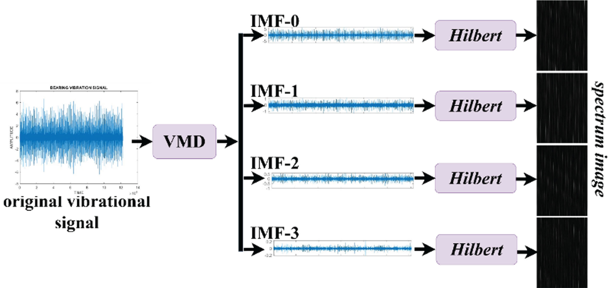
Hilbert spectrum creation of VMD-IMFs.

3.2 Dataset selection in bearing data

Experiments were carried out on the CWRU [62] bearing vibration signal database to demonstrate the effectiveness of our methodology. The experimental setup includes a dynamometer, a torque transducer, and a 2 HP motor. The motor shaft is supported by the test bearings. Electro-discharge machining is being used on the test bearings to create single-point defects with dimensions of 7, 14, 21, and 28 mils (one mil is equal to 0.001 inch). Digital data were recorded at a rate of 12,000 pulses per second for drive-end bearing problems. Speed and horsepower had to be manually recorded and measured by the torque transducer. Accelerometers will be used to collect vibration data. The bearing vibration signal database contains information on a wide range of signal elements. It covers a variety of fault types that might occur in experiment equipment, including inner race (IR), ball (BA), and orthogonal (OR) defects. The normal signal and all the classes of fault signals were considered in this experiment. Drive end (DE) accelerometer data is used in the proposed experiment to analyses the vibration signals corresponding to normal conditions and other defects. Following the procedures as discussed in Subsection 3.1 the original DE vibration signals from the bearing dataset are divided into M components and R IMF signals are obtained using EMD and VMD. The first four IMF signals are subsequently taken into focus, and the Hilbert transform is applied to each IMF signal before being transformed to image data with N = 256, resulting in 1105 × 4 images representing various faults for IMF₀ as shown in Table 1 similarly for IMF₁, IMF₂, and IMF₃. Figures 5 and 6 show a sample of 10 classes of erroneous spectrum images for the IMF₀ for EMD and VMD. These are visuals that were obtained for 10 different faulty classes and DCNN can further classify these images. Thus, in this case, there are four DCNN trained, and if the output is decided based on a voting mechanism the scheme will be similar to EL. More light on this shall be thrown in the result and discussion Section 5.

Fig. 5

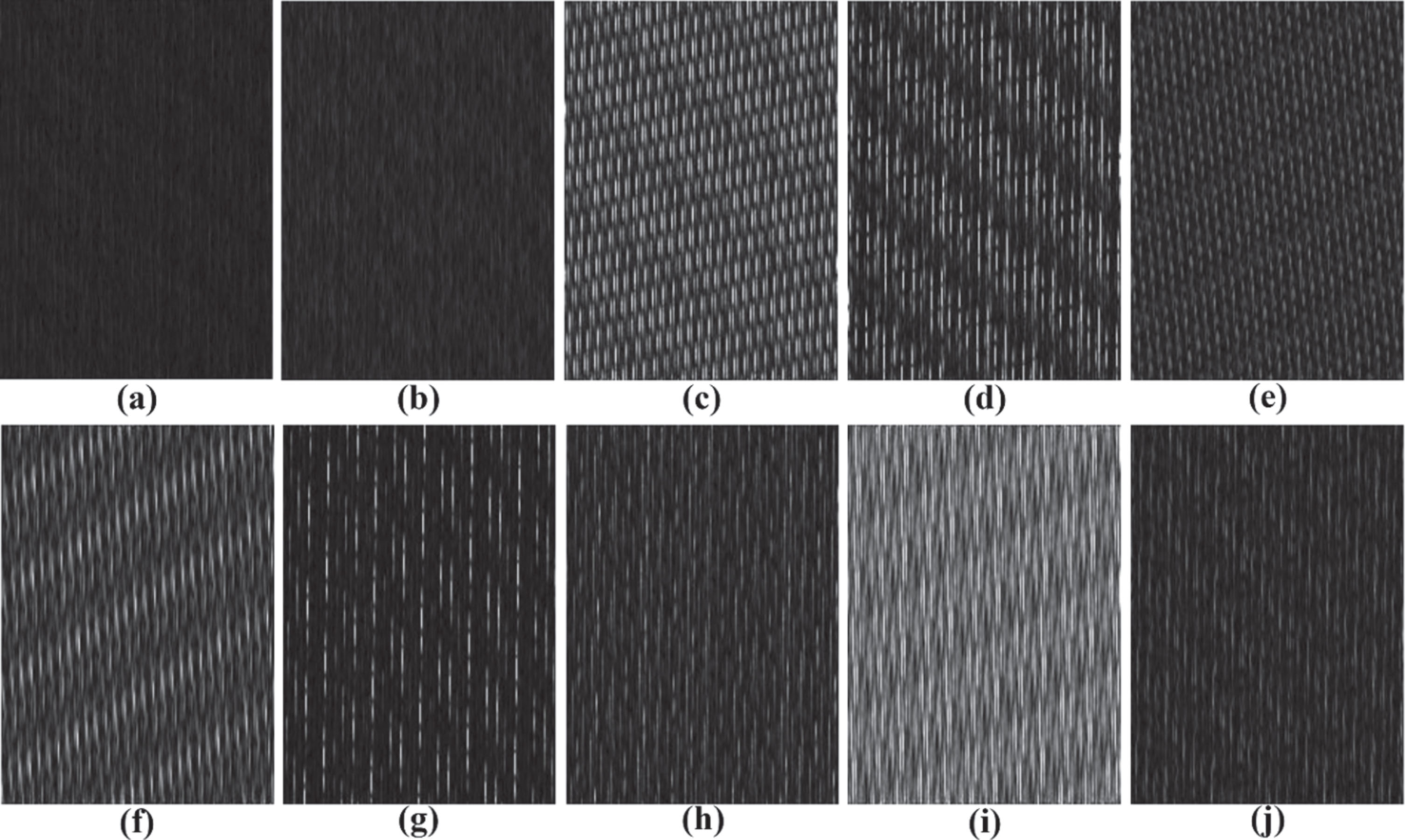
Sample EMD Hilbert spectrums for 10 different fault classes for CWRU bearing dataset (a) Ball B007, (b) Ball B021, (c) Centered OR007, (d) Centered OR021, (e) Inner Race IR007, (f) Inner race IR021, (g) Opposite OR007, (h) Opposite OR021, (i) Orthogonal OR007, (j) Orthogonal OR021.

Fig. 6

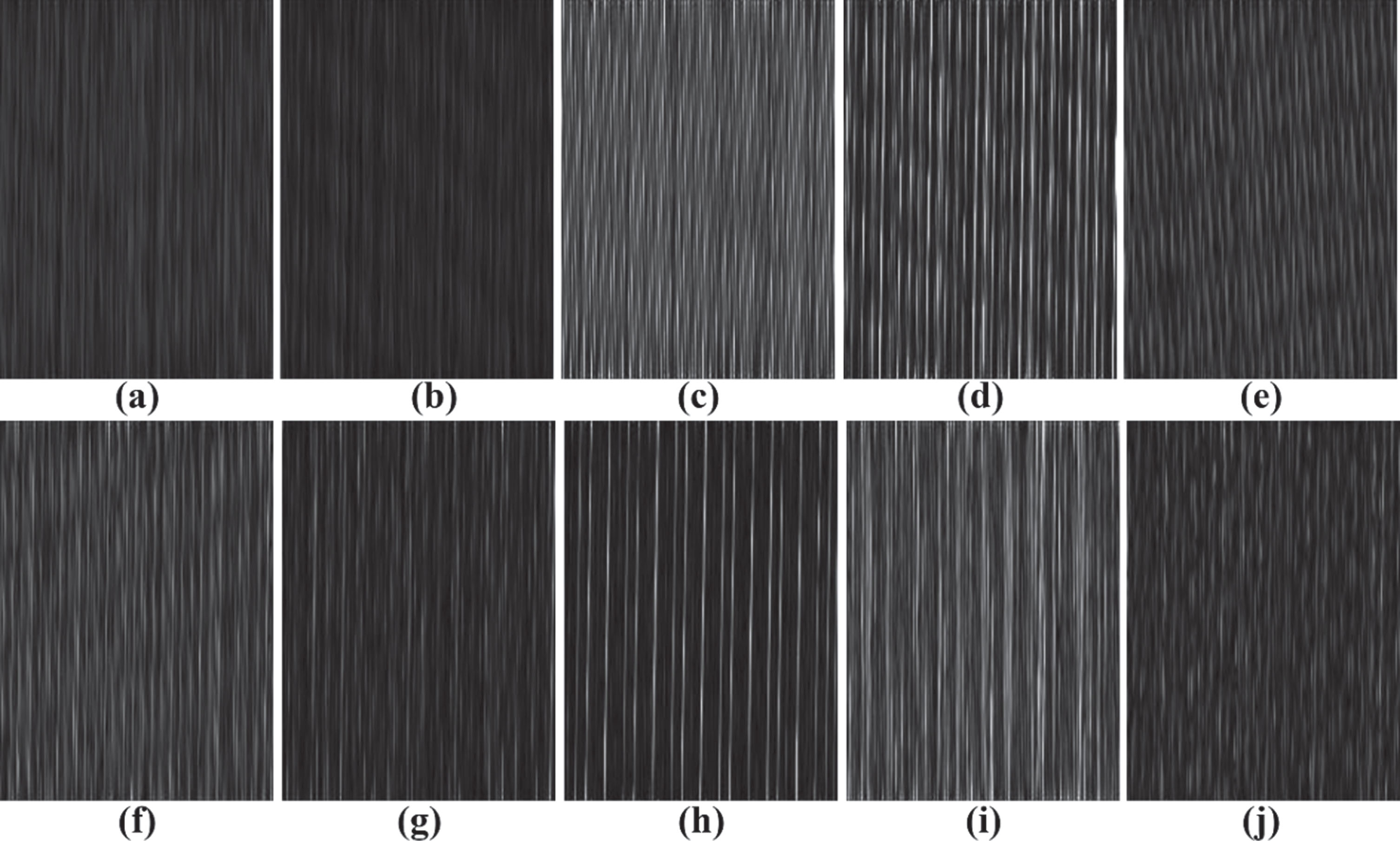
Sample VMD Hilbert spectrums for 10 different fault classes for CWRU bearing dataset (a) Ball B007, (b) Ball B021, (c) Centered OR007, (d) Centered OR021, (e) Inner Race IR007, (f) Inner race IR021, (g) Opposite OR007, (h) Opposite OR021, (i) Orthogonal OR007, (j) Orthogonal OR021.

Table 1

Configuration of the multi-class bearing dataset illustrated for IMF₀

Bearing-EMD &VMD (intrinsic mode function IMF)	IMF₀	IMF₀	IMF₀	IMF₀	IMF₀	IMF₀	IMF₀	IMF₀	IMF₀	IMF₀
Fault name	Inner Race IR007 3	Ball B007 3	Centered OR007@6 3	Orthogonal OR007@3 3	Opposite OR007@12 3	Inner race IR021 3	Ball B021 3	Centered OR021@6 3	Orthogonal OR021@3 3	Opposite OR021@12 3
Total images	1100	1096	1100	1099	1103	1096	1102	1105	1100	1108
Training (80%)	880	876	880	879	882	876	881	884	880	886
Testing (20%)	220	220	220	220	221	220	221	221	220	222

3.3 Dataset selection in milling data

Milling data [63] is another dataset that is more non-stationary in nature and used in this research to show the effectiveness of the proposed approach. The 167 struct array including the elements such as Case, Run, VB, Time, DOC, Feed, Material, smcAC, smcDC, Vib_Table, Vib_Spindle, and AE_Table and AE_Spindle lets up the milling data. This struct array is made up of 167 recordings from the experiment, and we use the vibration data from the vib-spindle to analyse it. The VB data for each recording indicates the tool’s flank wear and tear after the experiment. We took into account two examples in our analysis, fault and normal. Data with less wear and tear are assumed to be normal class, while data with excessive wear and tear are considered faults class (equivalent to VB > 3).

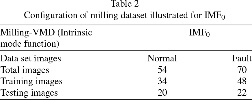
Following the procedures as discussed in Subsection 3.1 the original vibration signals from the bearing dataset are divided into M components and R IMF signals are obtained using EMD and VMD. The first four IMF signals are subsequently taken into focus, and Hilbert is applied to each IMF signal before being transformed to image data with N = 256, resulting in 54 × 4 images representing various faults for IMF₀ as shown in Table 2 similarly for IMF₁, IMF₂ and IMF₃.

Table 2
Configuration of milling dataset illustrated for IMF₀

Milling-VMD (Intrinsic IMF₀

mode function)

Data set images Normal Fault

Total images 54 70

Training images 34 48

Testing images 20 22

Milling-VMD (Intrinsic	IMF₀
Data set images	Normal	Fault
Total images	54	70
Training images	34	48
Testing images	20	22

Table 3

Model parameters of DCNN

Parameters	Values
Filter size	32 × 32, 64 × 64,
Batch size	32
Kernel size	3 × 3
Shear range	0.2
Zoom range	0.2
Layers	Conv2D, Max Pooling2D, Global AveragePooling2D, Dropout, Flatten, Dense
Activation layer	Relu, Softmax
Model type	Sequential
Optimizer	Adam
Flip type	Horizontal
Metrics	Accuracies
Loss function	Categorical-cross entropy
Epoch	25–100
Dense	256
Dropout	0.5

3.4 Statistical analysis of the vibration signal of the dataset

To prove that VMD analysis is better than EMD analysis the milling dataset which is more nonstationary in nature than the bearing dataset is used. This is because the IMF components of VMD analysis are free of aliasing noise. To show the nonstationary nature of the milling dataset a statistical analysis of each vibration signal is done. Vibration signals in the milling dataset are divided into good and bad vibration sets. For a given set the vibration signal is separated into consecutive frames and the mean is calculated for every frame and stored as a row in a matrix. This is done for every vibration signal and the matrix is filled. Thus, two different matrices are obtained for two different sets of good and fault. This matrix represents how the mean varies across the time for every vibration signal. The surf plot for the matrices is obtained & plotted in Fig. 7. From the surf plot, it can be observed that the variation of the mean value is large (maximum of 15*1031). Similarly, the experiment is done for different classes of bearing data, as shown in Fig. 8 and it can be observed the values range up to 0.05. This scale indicates that the variation of the mean across time is much larger for milling data than that for bearing data from which we can infer milling dataset is more nonstationary in nature.

Fig. 7

Surf plot of milling dataset statistical analysis (a) Good data (b) Bad data.

Fig. 8

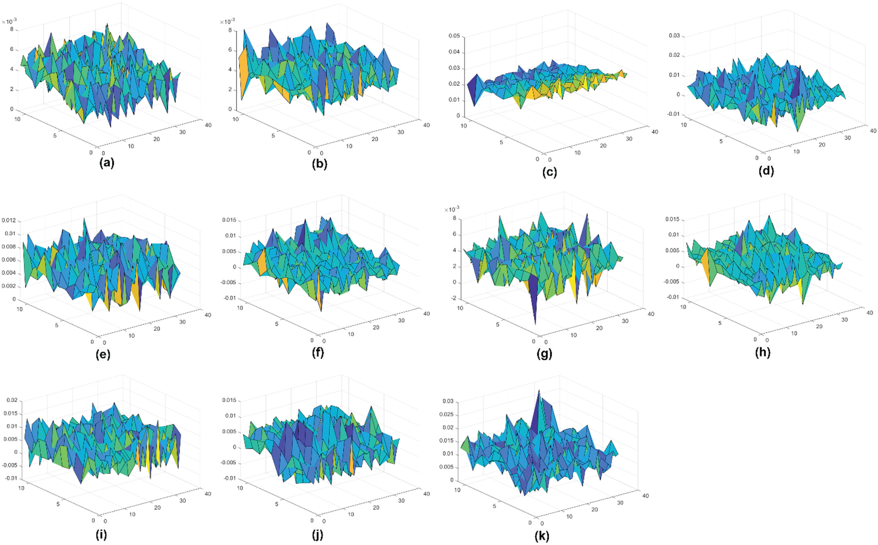
Surf plot of bearing dataset statistical analysis for 10 fault classes and normal (a) ball-0.007, (b) ball-0.21, (c) centered-0.007, (d) centered-0.21, (e) inner race-0.007, (f) inner race-0.21, (g) oppo-site-0.007, (h) opposite-0.21, (i) orthogonal-0.007, (j) orthogonal-0.21, (k) normal.

4 Data-driven model

The numerical demonstration works well with DCNN because the method uses images for categorization. A CNN is a feed-forward neural network that preserves the real connections between neurons. It is carried out based on the neurological system of living beings and now has implications for artificial intelligence, recommendation systems, and the processing of natural language. Consequently, convolutional filters learn the characteristics of the images automatically, and CNN is a technique with a remarkable ability to learn features reliably and sensitively. The CNN architecture comprises three layers: a convolutional layer, a sub-sampling layer, and a fully connected layer. Using one of the gradient-based optimization techniques, the parameters of the proposed model were computed. For a faster convergence, the parameters were updated using the Adam optimizer. The proposed deep CNN model contains two convolutional layers with 64, (3) and 128, (3) filters, respectively, as shown in Fig. 9. Two max-pooling layers with 2×2 pooling sizes were also utilized. Before being fed into the CNN model, the input photographs are resized to 64×64 pixels. The ReLU (Rectified Linear Units) activation function was used to incorporate nonlinearity at each level, enabling CNN to train sophisticated models. The suggested model was able to distinguish between the dominant and low-level features during training and classify texture images using a fully connected layer.

Fig. 9

DCNN architecture.

5 Results and discussion

In this study, we proposed to represent vibration signals as images and apply DCNN directly on the images, eliminating the feature extraction signal processing block. We investigated the method of using the Hilbert transform as an image representation technique. Hilbert imaging is performed in ways on the IMF signals obtained using VMD and empirical mode decomposition (EMD). The images obtained are used to train the DCNN to classify the faulty signal and the experiment is conducted on ten different fault data to bring out good models with better training and validation accuracies. This research shows the merits of VMD and EMD based imaging. As already discussed, it is proposed to use EMD analysis and VMD analysis on two different datasets the bearing data set and milling data set which is more non-stationary than the bearing data set as illustrated in Subsection 3.4.

5.1 Inference from DCNN learning of bearing dataset

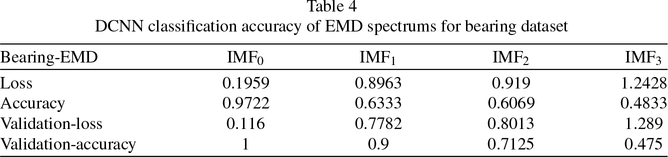
The training and testing samples are given in Table 1. The CNN learning is applied to the bearing dataset as shown in Table 1 for both the set of EMD and VMD IMFs based spectrums and the performance metrics of the ML model are shown in Tables 4&5 respectively. From Table 4 it can be inferred that among the four EMD-IMFs, EMD-IMF₀ based spectrums ML model has a training accuracy of 0.9722 with a validation accuracy of 1. From Table 5 it can be inferred that among four VMD- IMFs both IMF₀ & IMF₁ based spectrums ML model have validation accuracy of 1 thanks to aliasing free VMD-IMF components.

Table 4
DCNN classification accuracy of EMD spectrums for bearing dataset

Bearing-EMD IMF₀ IMF₁ IMF₂ IMF₃

Loss 0.1959 0.8963 0.919 1.2428

Accuracy 0.9722 0.6333 0.6069 0.4833

Validation-loss 0.116 0.7782 0.8013 1.289

Validation-accuracy 1 0.9 0.7125 0.475

Bearing-EMD	IMF₀	IMF₁	IMF₂	IMF₃
Loss	0.1959	0.8963	0.919	1.2428
Accuracy	0.9722	0.6333	0.6069	0.4833
Validation-loss	0.116	0.7782	0.8013	1.289
Validation-accuracy	1	0.9	0.7125	0.475

Table 5

DCNN classification accuracy of VMD spectrums for bearing dataset

Bearing-VMD	IMF₀	IMF₁	IMF₂	IMF₃
Loss	0.4882	0.3869	0.4775	0.5743
Accuracy	0.8708	0.8806	0.8081	0.7819
Validation-loss	0.3945	0.2876	0.3621	0.4932
Validation-accuracy	1	1	0.85	0.85

Table 4 summarizes the CNN model learning accuracy results for the bearing data dataset images shown in Table 1. Figure 10 displays the model accuracy and validation accuracy for all EMD IMFs of the bearing dataset for the epoch. Figure 11 depicts the confusion matrix for all EMD IMFs for a random experiment.

Fig. 10

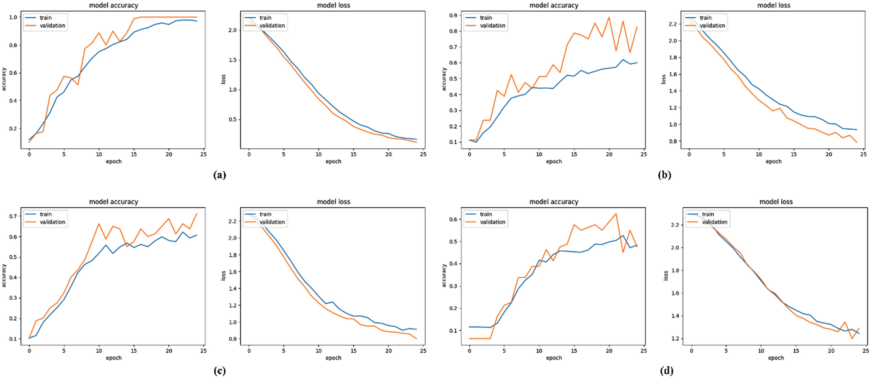
DCNN model accuracies and loss against epoch for EMD analysis of bearing dataset (a) IMF₀, (b) IMF₁, (c) IMF₂, (d) IMF₃.

Fig. 11

DCNN model confusion-matrix for EMD analysis of bearing dataset (a) IMF₀, (b) IMF₁, (c) IMF₂, (d) IMF₃.

Table 5 summarizes the CNN model learning accuracy results for the bearing data dataset images shown in Table 1. Figure 12 displays the model accuracy and validation accuracy for all VMD IMFs of the bearing dataset for the epoch. Figure 13 depicts the confusion matrix for all VMD IMFs for a random experiment.

Fig. 12

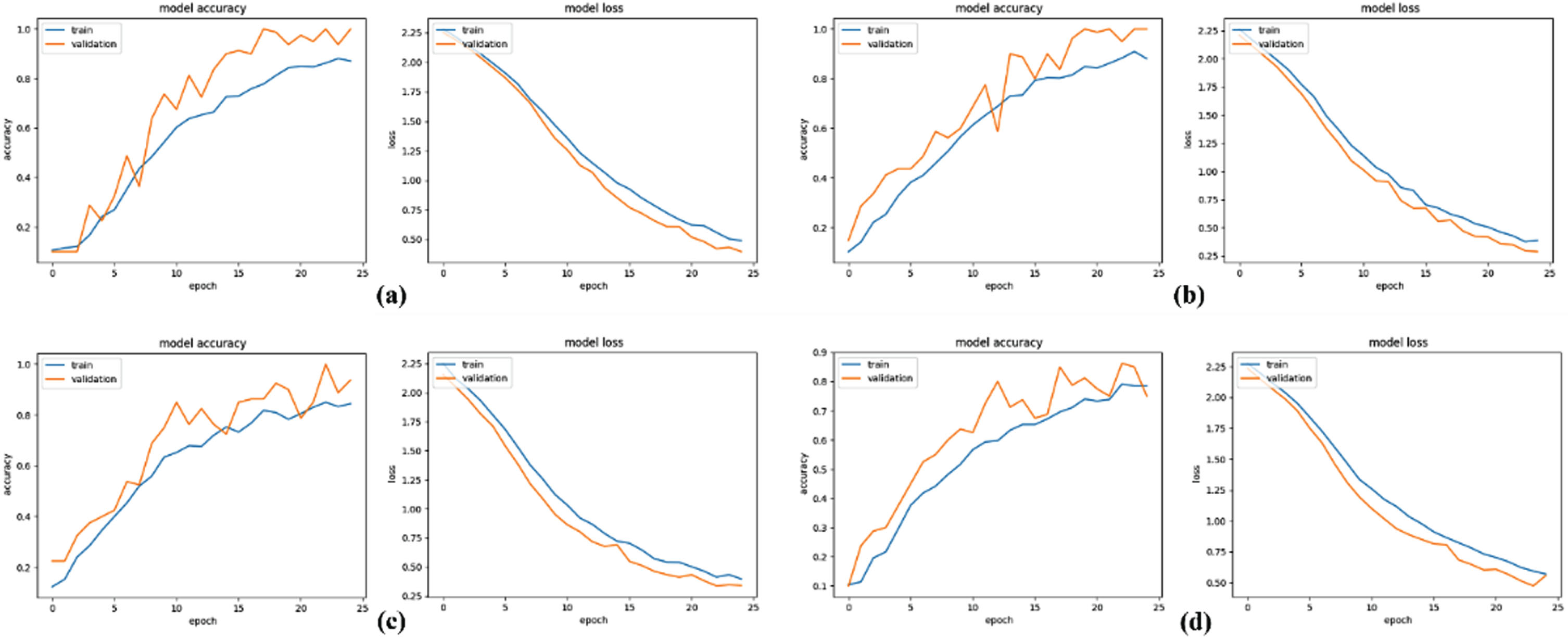
DCNN model accuracies and loss against epoch for VMD analysis of bearing dataset (a) IMF₀, (b) IMF₁, (c) IMF₂, (d) IMF₃.

Fig. 13

DCNN model confusion-matrix for VMD analysis of bearing dataset (a) IMF₀, (b) IMF₁, (c) IMF₂, (d) IMF₃.

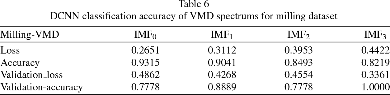
5.2 Inference from DCNN learning of milling dataset

To bring out the performance improvement of VMD analysis for non-stationary signals the milling dataset is considered. In a recent work [32] EMD analysis of a milling dataset results in an ML model with a validation accuracy of 0.8125 for the IMF₀ spectrum. The CNN learning is applied to the milling dataset as shown in Table 2 for the set of VMD IMFs based spectrums and the performance metrics of the ML model are shown in Table 6. From Table 6 it can be inferred that among four IMFs both IMF₁ and IMF₃ based spectrums ML model has validation accuracy of 0.888 and 1.0 respectively thanks to aliasing free IMF components.

Table 6
DCNN classification accuracy of VMD spectrums for milling dataset

Milling-VMD IMF₀ IMF₁ IMF₂ IMF₃

Loss 0.2651 0.3112 0.3953 0.4422

Accuracy 0.9315 0.9041 0.8493 0.8219

Validation_loss 0.4862 0.4268 0.4554 0.3361

Validation-accuracy 0.7778 0.8889 0.7778 1.0000

Milling-VMD	IMF₀	IMF₁	IMF₂	IMF₃
Loss	0.2651	0.3112	0.3953	0.4422
Accuracy	0.9315	0.9041	0.8493	0.8219
Validation_loss	0.4862	0.4268	0.4554	0.3361
Validation-accuracy	0.7778	0.8889	0.7778	1.0000

Table 6 summarizes the CNN model learning accuracy results for the milling data dataset images shown in Table 2. Figure 14 displays the model accuracy and validation accuracy for all VMD IMFs of the milling dataset for the epoch.

Fig. 14

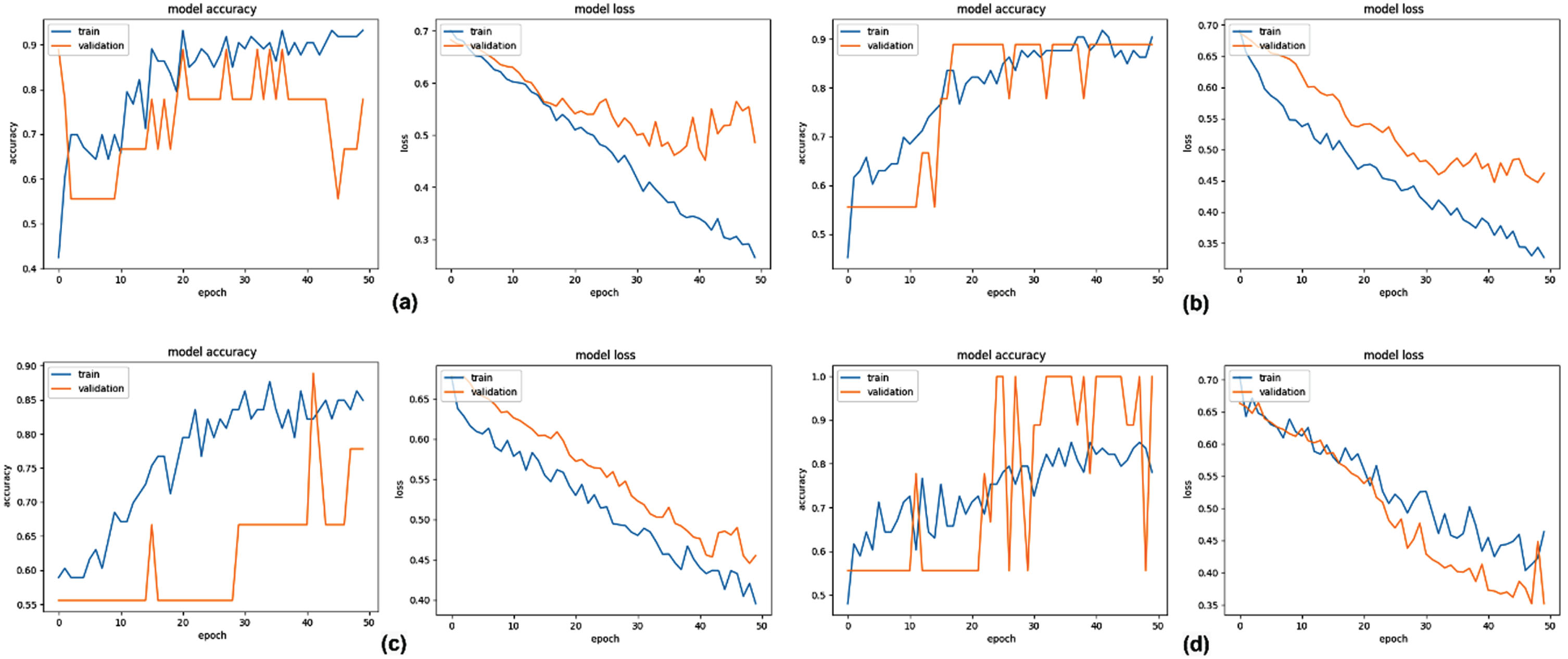
DCNN model accuracies and loss against epoch for VMD analysis of milling dataset (a) IMF₀, (b) IMF₁, (c) IMF₂, (d) IMF₃.

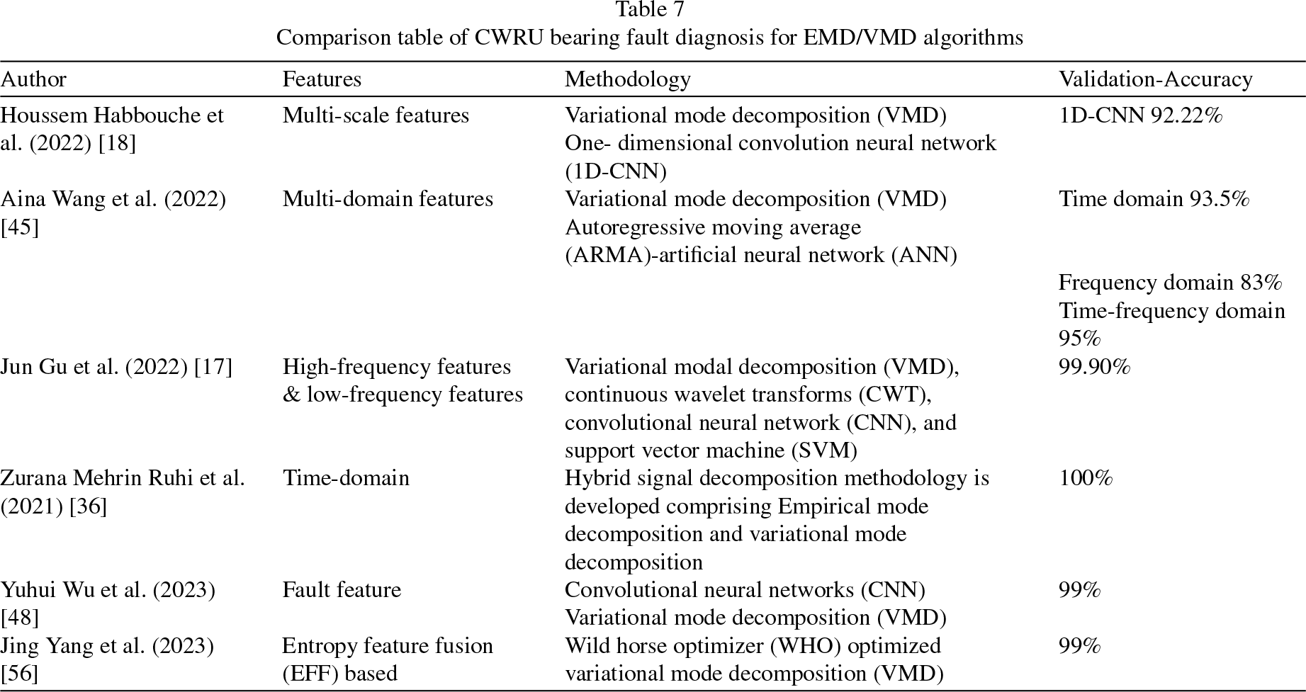
5.3 Performance of EMD/VMD based benchmark methods

In this present paper, the Hilbert spectrum images of IMFs of EMD/VMD signals of the CWRU bearing dataset are proposed for DCNN learning. The performance of EMD/VMD benchmark methods done on this bearing dataset is given in Table 7. In the present paper, both EMD/VMD spectrum based DCNN method being 100% validation accuracy (Tables 4 and 5) are on par or exceeds the performance of benchmark methods given in Table 7.

Table 7
Comparison table of CWRU bearing fault diagnosis for EMD/VMD algorithms

Author Features Methodology Validation-Accuracy

Houssem Habbouche et al. (2022) [18] Multi-scale features Variational mode decomposition (VMD) One- dimensional convolution neural network (1D-CNN) 1D-CNN 92.22%

Aina Wang et al. (2022) [45] Multi-domain features Variational mode decomposition (VMD) Autoregressive moving average (ARMA)-artificial neural network (ANN) Time domain 93.5%

Frequency domain 83%

Time-frequency domain 95%

Jun Gu et al. (2022) [17] High-frequency features &low-frequency features Variational modal decomposition (VMD), continuous wavelet transforms (CWT), convolutional neural network (CNN), and support vector machine (SVM) 99.90%

Zurana Mehrin Ruhi et al. (2021) [36] Time-domain Hybrid signal decomposition methodology is developed comprising Empirical mode decomposition and variational mode decomposition 100%

Yuhui Wu et al. (2023) [48] Fault feature Convolutional neural networks (CNN) Variational mode decomposition (VMD) 99%

Jing Yang et al. (2023) [56] Entropy feature fusion (EFF) based Wild horse optimizer (WHO) optimized variational mode decomposition (VMD) 99%

Author	Features	Methodology	Validation-Accuracy
Houssem Habbouche et al. (2022) [18]	Multi-scale features	Variational mode decomposition (VMD) One- dimensional convolution neural network (1D-CNN)	1D-CNN 92.22%
Aina Wang et al. (2022) [45]	Multi-domain features	Variational mode decomposition (VMD) Autoregressive moving average (ARMA)-artificial neural network (ANN)	Time domain 93.5%
			Frequency domain 83%
			Time-frequency domain 95%
Jun Gu et al. (2022) [17]	High-frequency features &low-frequency features	Variational modal decomposition (VMD), continuous wavelet transforms (CWT), convolutional neural network (CNN), and support vector machine (SVM)	99.90%
Zurana Mehrin Ruhi et al. (2021) [36]	Time-domain	Hybrid signal decomposition methodology is developed comprising Empirical mode decomposition and variational mode decomposition	100%
Yuhui Wu et al. (2023) [48]	Fault feature	Convolutional neural networks (CNN) Variational mode decomposition (VMD)	99%
Jing Yang et al. (2023) [56]	Entropy feature fusion (EFF) based	Wild horse optimizer (WHO) optimized variational mode decomposition (VMD)	99%

5.4 Performance of ensemble learning method

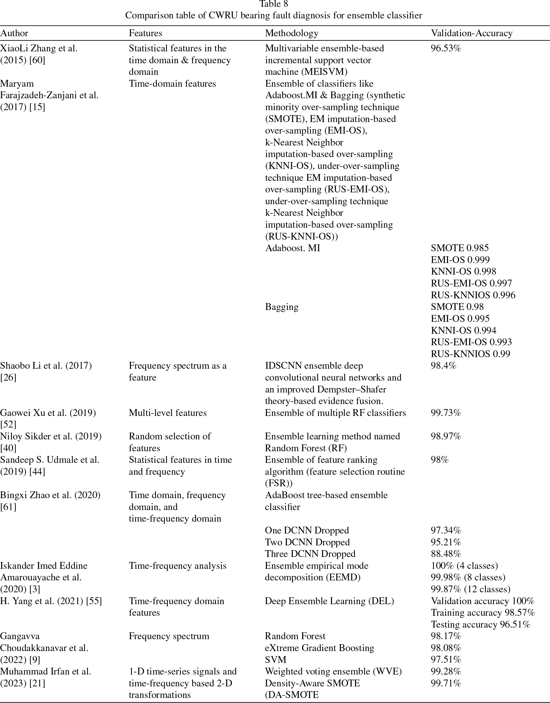
As already we discussed, the proposed method involves multiple CNNs (4 in number) and if a voting system is used to select the best output this scheme will be similar to EL. The performance of EL based benchmark methods done on this bearing dataset is given in Table 8. In the present paper, both EMD/VMD spectrum based DCNN method being 100% validation accuracy (Tables 4 and 5) are on par or exceeds the performance of benchmark EL methods given in Table 8. Though the present method is similar to EL method in terms of multiple CNN training, it is actually different from EL methods as there is no voting mechanism. Among four CNN one of the CNN is 100% accurate as given in Table 5 the need for a voting scheme is eliminated. But in future in a constrained noisy environment the EL learning can be applied in this scenario. It should be noted that the proposed problem is done for multi-class classification and 100% validation accuracy CWRU bearing dataset for IMF₀ and IMF₁ implies that both IMF₀ and IMF₁ signals generalize all different 10 faults assumed in this work and for the final deployment either of these models can be used. In case none of the IMF signals gives 100% accuracy a voting scheme is required. It should also be noted that for the non-stationary milling dataset, 100% accuracy is observed for IMF₃ signals. The merit of the proposed algorithm is that it needs only one CNN model which is the best model to be deployed finally minimizing the memory and computation cost.

Table 8
Comparison table of CWRU bearing fault diagnosis for ensemble classifier

Author Features Methodology Validation-Accuracy

XiaoLi Zhang et al. (2015) [60] Statistical features in the time domain &frequency domain Multivariable ensemble-based incremental support vector machine (MEISVM) 96.53%

Maryam Farajzadeh-Zanjani et al. (2017) [15] Time-domain features Ensemble of classifiers like Adaboost.MI &Bagging (synthetic minority over-sampling technique (SMOTE), EM imputation-based over-sampling (EMI-OS), k-Nearest Neighbor imputation-based over-sampling (KNNI-OS), under-over-sampling technique EM imputation-based over-sampling (RUS-EMI-OS), under-over-sampling technique k-Nearest Neighbor imputation-based over-sampling (RUS-KNNI-OS))

Adaboost. MI SMOTE 0.985

EMI-OS 0.999

KNNI-OS 0.998

RUS-EMI-OS 0.997

RUS-KNNIOS 0.996

Bagging SMOTE 0.98

EMI-OS 0.995

KNNI-OS 0.994

RUS-EMI-OS 0.993

RUS-KNNIOS 0.99

Shaobo Li et al. (2017) [26] Frequency spectrum as a feature IDSCNN ensemble deep convolutional neural networks and an improved Dempster– Shafer theory-based evidence fusion. 98.4%

Gaowei Xu et al. (2019) [52] Multi-level features Ensemble of multiple RF classifiers 99.73%

Niloy Sikder et al. (2019) [40] Random selection of features Ensemble learning method named Random Forest (RF) 98.97%

Sandeep S. Udmale et al. (2019) [44] Statistical features in time and frequency Ensemble of feature ranking algorithm (feature selection routine (FSR)) 98%

Bingxi Zhao et al. (2020) [61] Time domain, frequency domain, and time-frequency domain AdaBoost tree-based ensemble classifier

One DCNN Dropped 97.34%

Two DCNN Dropped 95.21%

Three DCNN Dropped 88.48%

Iskander Imed Eddine Amarouayache et al. (2020) [3] Time-frequency analysis Ensemble empirical mode decomposition (EEMD) 100% (4 classes) 99.98% (8 classes) 99.87% (12 classes)

H. Yang et al. (2021) [55] Time-frequency domain features Deep Ensemble Learning (DEL) Validation accuracy 100% Training accuracy 98.57% Testing accuracy 96.51%

Gangavva Choudakkanavar et al. (2022) [9] Frequency spectrum Random Forest eXtreme Gradient Boosting SVM 98.17% 98.08% 97.51%

Muhammad Irfan et al. (2023) [21] 1-D time-series signals and time-frequency based 2-D transformations Weighted voting ensemble (WVE) Density-Aware SMOTE (DA-SMOTE 99.28% 99.71%

Author	Features	Methodology	Validation-Accuracy
XiaoLi Zhang et al. (2015) [60]	Statistical features in the time domain &frequency domain	Multivariable ensemble-based incremental support vector machine (MEISVM)	96.53%
Maryam Farajzadeh-Zanjani et al. (2017) [15]	Time-domain features	Ensemble of classifiers like Adaboost.MI &Bagging (synthetic minority over-sampling technique (SMOTE), EM imputation-based over-sampling (EMI-OS), k-Nearest Neighbor imputation-based over-sampling (KNNI-OS), under-over-sampling technique EM imputation-based over-sampling (RUS-EMI-OS), under-over-sampling technique k-Nearest Neighbor imputation-based over-sampling (RUS-KNNI-OS))
		Adaboost. MI	SMOTE 0.985
			EMI-OS 0.999
			KNNI-OS 0.998
			RUS-EMI-OS 0.997
			RUS-KNNIOS 0.996
		Bagging	SMOTE 0.98
			EMI-OS 0.995
			KNNI-OS 0.994
			RUS-EMI-OS 0.993
			RUS-KNNIOS 0.99
Shaobo Li et al. (2017) [26]	Frequency spectrum as a feature	IDSCNN ensemble deep convolutional neural networks and an improved Dempster– Shafer theory-based evidence fusion.	98.4%
Gaowei Xu et al. (2019) [52]	Multi-level features	Ensemble of multiple RF classifiers	99.73%
Niloy Sikder et al. (2019) [40]	Random selection of features	Ensemble learning method named Random Forest (RF)	98.97%
Sandeep S. Udmale et al. (2019) [44]	Statistical features in time and frequency	Ensemble of feature ranking algorithm (feature selection routine (FSR))	98%
Bingxi Zhao et al. (2020) [61]	Time domain, frequency domain, and time-frequency domain	AdaBoost tree-based ensemble classifier
		One DCNN Dropped	97.34%
		Two DCNN Dropped	95.21%
		Three DCNN Dropped	88.48%
Iskander Imed Eddine Amarouayache et al. (2020) [3]	Time-frequency analysis	Ensemble empirical mode decomposition (EEMD)	100% (4 classes) 99.98% (8 classes) 99.87% (12 classes)
H. Yang et al. (2021) [55]	Time-frequency domain features	Deep Ensemble Learning (DEL)	Validation accuracy 100% Training accuracy 98.57% Testing accuracy 96.51%
Gangavva Choudakkanavar et al. (2022) [9]	Frequency spectrum	Random Forest eXtreme Gradient Boosting SVM	98.17% 98.08% 97.51%
Muhammad Irfan et al. (2023) [21]	1-D time-series signals and time-frequency based 2-D transformations	Weighted voting ensemble (WVE) Density-Aware SMOTE (DA-SMOTE	99.28% 99.71%

5.5 Comparison with state of art DCNN based method

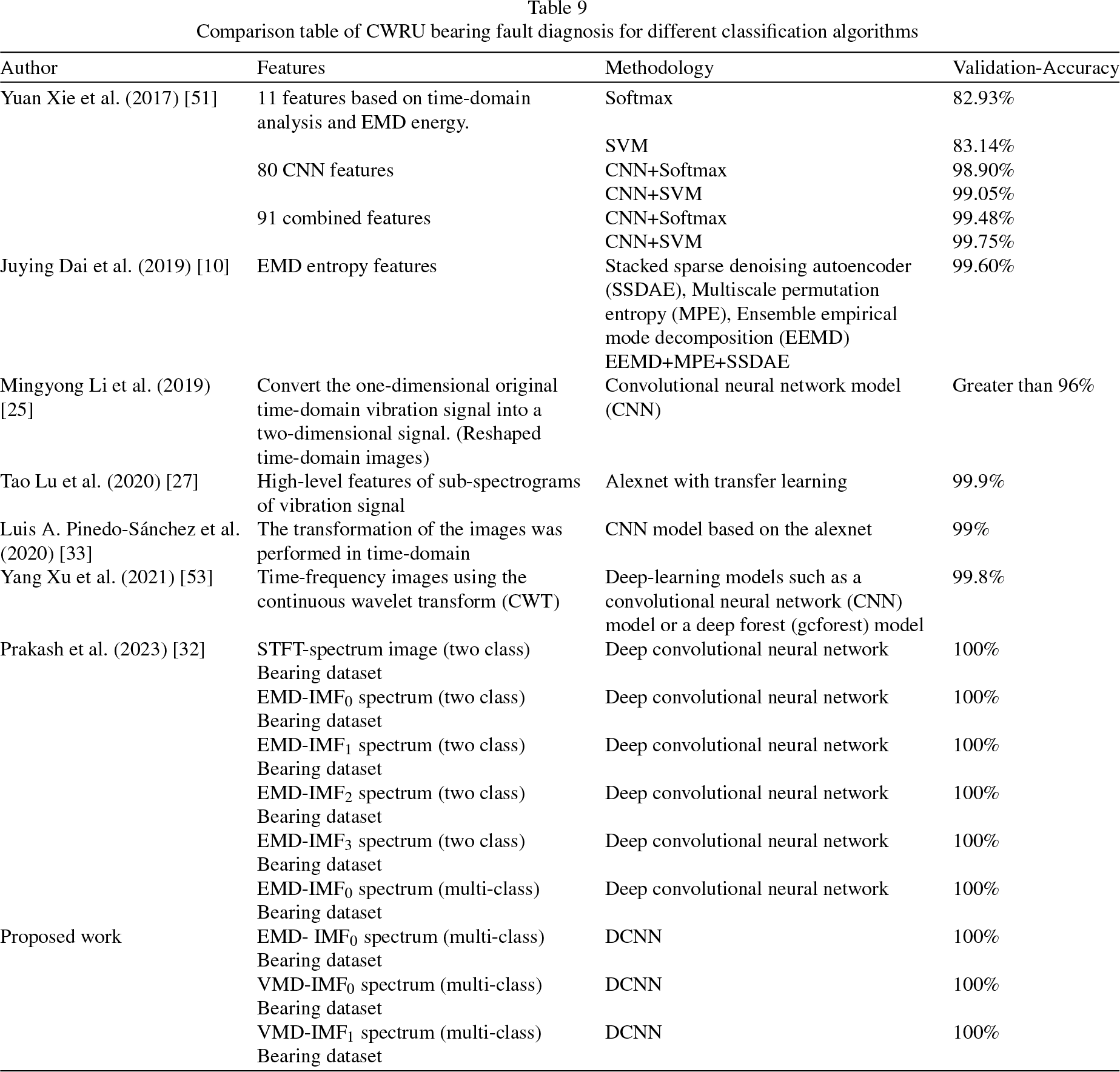
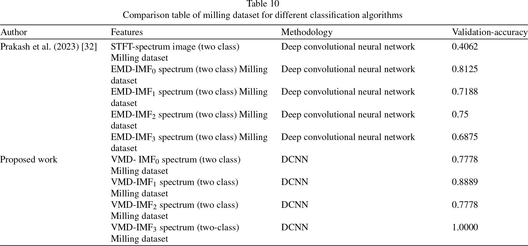
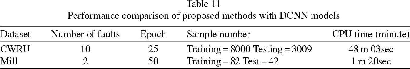
A comparison is given in Table 9 for the EMD and VMD methods done in this paper using DCNN benchmarked against state-of-the-art methods it can be observed that in DCNN VMD-based analysis outperforms for IMF₀ & IMF₁ and EMD-based analysis outperforms for IMF₀ for multi-class classification in terms of validation accuracy and Table 10 shows the comparison of milling dataset which is more non-stationary in nature for EMD and VMD algorithm. The spectrum of VMD-IMF₃ for two-class classification gives 100% validation accuracy and is much better than EMD analysis. Also, it can be seen that all approaches are improved by the VMD-based analysis working with DCNN in regards to validation accuracy. Table 11 shows the execution time of the proposed method with the DCNN model for bearing and milling datasets based on training and validation. The experiment is done in cloud platform and the system parameters are 11th Gen Intel(R) Core (TM) i5-1135G7 processor at a clock of 2.40 GHz with RAM of 8.00 GB, 64-bit operating system and Windows 11 with network band 2.4 GHz speed receiver/transmitter 144/144 (Mbps). The value mentioned is for the time taken for training and validation. The validation alone takes around 5 seconds and thus negligible.

Table 9
Comparison table of CWRU bearing fault diagnosis for different classification algorithms

Author Features Methodology Validation-Accuracy

Yuan Xie et al. (2017) [51] 11 features based on time-domain analysis and EMD energy. Softmax 82.93%

SVM 83.14%

80 CNN features CNN+Softmax 98.90%

CNN+SVM 99.05%

91 combined features CNN+Softmax 99.48%

CNN+SVM 99.75%

Juying Dai et al. (2019) [10] EMD entropy features Stacked sparse denoising autoencoder (SSDAE), Multiscale permutation entropy (MPE), Ensemble empirical mode decomposition (EEMD) EEMD+MPE+SSDAE 99.60%

Mingyong Li et al. (2019) [25] Convert the one-dimensional original time-domain vibration signal into a two-dimensional signal. (Reshaped time-domain images) Convolutional neural network model (CNN) Greater than 96%

Tao Lu et al. (2020) [27] High-level features of sub-spectrograms of vibration signal Alexnet with transfer learning 99.9%

Luis A. Pinedo-Sánchez et al. (2020) [33] The transformation of the images was performed in time-domain CNN model based on the alexnet 99%

Yang Xu et al. (2021) [53] Time-frequency images using the continuous wavelet transform (CWT) Deep-learning models such as a convolutional neural network (CNN) model or a deep forest (gcforest) model 99.8%

Prakash et al. (2023) [32] STFT-spectrum image (two class) Bearing dataset Deep convolutional neural network 100%

EMD-IMF₀ spectrum (two class) Bearing dataset Deep convolutional neural network 100%

EMD-IMF₁ spectrum (two class) Bearing dataset Deep convolutional neural network 100%

EMD-IMF₂ spectrum (two class) Bearing dataset Deep convolutional neural network 100%

EMD-IMF₃ spectrum (two class) Bearing dataset Deep convolutional neural network 100%

EMD-IMF₀ spectrum (multi-class) Bearing dataset Deep convolutional neural network 100%

Proposed work EMD- IMF₀ spectrum (multi-class) Bearing dataset DCNN 100%

VMD-IMF₀ spectrum (multi-class) Bearing dataset DCNN 100%

VMD-IMF₁ spectrum (multi-class) Bearing dataset DCNN 100%

Author	Features	Methodology	Validation-Accuracy
Yuan Xie et al. (2017) [51]	11 features based on time-domain analysis and EMD energy.	Softmax	82.93%
		SVM	83.14%
	80 CNN features	CNN+Softmax	98.90%
		CNN+SVM	99.05%
	91 combined features	CNN+Softmax	99.48%
		CNN+SVM	99.75%
Juying Dai et al. (2019) [10]	EMD entropy features	Stacked sparse denoising autoencoder (SSDAE), Multiscale permutation entropy (MPE), Ensemble empirical mode decomposition (EEMD) EEMD+MPE+SSDAE	99.60%
Mingyong Li et al. (2019) [25]	Convert the one-dimensional original time-domain vibration signal into a two-dimensional signal. (Reshaped time-domain images)	Convolutional neural network model (CNN)	Greater than 96%
Tao Lu et al. (2020) [27]	High-level features of sub-spectrograms of vibration signal	Alexnet with transfer learning	99.9%
Luis A. Pinedo-Sánchez et al. (2020) [33]	The transformation of the images was performed in time-domain	CNN model based on the alexnet	99%
Yang Xu et al. (2021) [53]	Time-frequency images using the continuous wavelet transform (CWT)	Deep-learning models such as a convolutional neural network (CNN) model or a deep forest (gcforest) model	99.8%
Prakash et al. (2023) [32]	STFT-spectrum image (two class) Bearing dataset	Deep convolutional neural network	100%
	EMD-IMF₀ spectrum (two class) Bearing dataset	Deep convolutional neural network	100%
	EMD-IMF₁ spectrum (two class) Bearing dataset	Deep convolutional neural network	100%
	EMD-IMF₂ spectrum (two class) Bearing dataset	Deep convolutional neural network	100%
	EMD-IMF₃ spectrum (two class) Bearing dataset	Deep convolutional neural network	100%
	EMD-IMF₀ spectrum (multi-class) Bearing dataset	Deep convolutional neural network	100%
Proposed work	EMD- IMF₀ spectrum (multi-class) Bearing dataset	DCNN	100%
	VMD-IMF₀ spectrum (multi-class) Bearing dataset	DCNN	100%
	VMD-IMF₁ spectrum (multi-class) Bearing dataset	DCNN	100%

Table 10

Comparison table of milling dataset for different classification algorithms

Author	Features	Methodology	Validation-accuracy
Prakash et al. (2023) [32]	STFT-spectrum image (two class) Milling dataset	Deep convolutional neural network	0.4062
	EMD-IMF₀ spectrum (two class) Milling dataset	Deep convolutional neural network	0.8125
	EMD-IMF₁ spectrum (two class) Milling dataset	Deep convolutional neural network	0.7188
	EMD-IMF₂ spectrum (two class) Milling dataset	Deep convolutional neural network	0.75
	EMD-IMF₃ spectrum (two class) Milling dataset	Deep convolutional neural network	0.6875
Proposed work	VMD- IMF₀ spectrum (two class) Milling dataset	DCNN	0.7778
	VMD-IMF₁ spectrum (two class) Milling dataset	DCNN	0.8889
	VMD-IMF₂ spectrum (two class) Milling dataset	DCNN	0.7778
	VMD-IMF₃ spectrum (two-class) Milling dataset	DCNN	1.0000

Table 11

Performance comparison of proposed methods with DCNN models

Dataset	Number of faults	Epoch	Sample number	CPU time (minute)
CWRU	10	25	Training = 8000 Testing = 3009	48 m 03sec
Mill	2	50	Training = 82 Test = 42	1 m 20sec

5.6 Key inference points

By analysing all the results discussed above, the following are the key inference points that are derived from the numerical experiment done for

–
Unlike using the energy and entropy parameters of EMD-IMFs of a vibration signal to classify machine faults a different approach is used in which spectrogram images of IMF signal are used in DCNN learning.
–
It is proposed to bring out the merits of aliasing free VMD-IMF over EMD-IMF and it is shown that the validation accuracy of all the four IMFs is better for VMD over EMD. Two of the VMD-IMFs IMF₀ and IMF₁ result in an 100% validation accuracy.
–
To further bring out the robustness of the VMD approach, VMD is applied to the milling dataset which is the more non-stationary bearing dataset. The result obtained is 100% validation accuracy for IMF₃ which is better than the EMD method of 81% validation accuracy shown in our recent work [32].
–
The merits of the proposed VMD approach over the EL approach are that the proposed approach uses the best IMF function that gives 100% validation accuracy and needs only one CNN model to be deployed in the application.

6 Conclusions

Numerical experiments are conducted to determine the efficacy of VMD analysis of vibration signals using DCNN to classify machine faults. The idea of representing IMF components obtained by EMD and VMD as Hilbert spectral images and trained in DCNN to classify the machine faults is demonstrated using CWRU bearing dataset for 10 different fault classes. The model accuracies are tabulated and plotted against the epochs. The results show that one of the four IMFs (IMF₀) of the EMD method gives a validation accuracy of 100% and two of the four IMFs (IMF_0 & IMF₁) of the VMD method give a validation accuracy of 100%. It is also shown that the validation accuracy of all four IMFs of VMD is better than the EMD method. The confusion matrix is obtained and depicted for this 10-class problem which also supports that VMD based analysis is better than EMD based analysis. To substantiate this statement, the VMD based DCNN experiment is repeated for a different non-stationary dataset (milling dataset) for a binary class problem and it is shown that the IMF₃ component gives an accuracy of 100% which is very high for an EMD based method demonstrated using DCNN in previous work for the same dataset with a maximum validation accuracy of 81%. The proposed method is compared with the state-of-the-art work and it is evident that VMD based analysis outperforms all other methods. It is also better than the popular EL algorithm as it requires the deployment of one single best model in the application end. The future scope identified for this work is to extend the idea for noisy vibration signals by optimally searching the best possible number of IMFs using heuristic algorithms and to fuse the best results for a better outcome in an EL based framework.

References

Aherwar

Khalid

Vibration analysis techniques for gearbox diagnostic: A review, Int. J. Adv. Eng. Technol.3 (2012), 4–12.

Ahmadi

Ekhlasi

Types of EMD algorithms, , 5th Iran. Conf. Signal Process. Intell. Syst. ICSPIS2019 (2019), 18–19.

Amarouayache

I.I.E.

Saadi

M.N.

Guersi

Boutasseta

Bearing fault diagnostics using EEMD processing and convolutional neural network methods, , Int. J. Adv. Manuf. Technol.107 (2020), 4077–4095.

Asilturk

Aslanci

Ozmen

Machinery monitoring using vibration signal analysis,, 40th IASTEM Int. Conf. Kuala Lumpur, Malaysia (2016), 978–93.

Baba Fakruddin Ali

B.H.

, Ramachandran,

Compressive wavelet domain deep CNN for image classification using genetic algorithm based sensing mask learning, , IEEE Access.11 (2023), 35567–35578.

Shao

Wang

Lai

Prediction of coal mine gas emission based on hybrid machine learning model, , Earth Sci. Informatics.16 (2023), 501–513.

Shao

Zheng

Yang

Workshop layout optimization method based on sparrow search algorithm: a new approach,, J. Ind. Prod. Eng. (2024).

Cai

Zhang

Xie

Tool vibration feature extraction method based on SSA-VMD and SVM,, Arab. J. Sci. Eng. (2022).

Choudakkanavar

Mangai

J.A.

Bansal

MFCC based ensemble learning method for multiple fault diagnosis of roller bearing, , Int. J. Inf. Technol.14 (2022), 2741–2751.

10.

Dai

Tang

Shao

Huang

Wang

Fault diagnosis of rolling bearing based on multiscale intrinsic mode function permutation entropy and a stacked sparse denoising autoencoder, , Appl. Sci.9 (2019).

11.

Dekys

Condition monitoring and fault diagnosis, , Procedia Eng.177 (2017), 502–509.

12.

Dhamande

L.S.

Chaudhari

M.B.

Compound gear-bearing fault feature extraction using statistical features based on time-frequency method, , Meas. J. Int. Meas. Confed.125 (2018), 63–77.

13.

Yang

Application of the EMD method in the vibration analysis of ball bearings, , Mech. Syst. Signal Process21 (2007), 2634–2644.

14.

Fan

Shao

Zhang

Wan

Cao

Intelligent Fault Diagnosis of Rolling Bearing Using FCM Clustering of EMD-PWVD Vibration Images, , IEEE Access8 (2020), 145194–145206.

15.

Farajzadeh-Zanjani

Razavi-Far

Saif

Efficient sampling techniques for ensemble learning and diagnosing bearing defects under class imbalanced condition, , 2016 IEEE Symp. Ser. Comput. Intell. SSCI2016 (2017), 1–7.

16.

González-Muñiz

Díaz

Cuadrado

A.A.

DCNN forcondition monitoring and fault detection in rotating machines andits contribution to the understanding of machine nature, Heliyon6 (2020), e03395.

17.

Peng

Chang

Chen

A novel fault diagnosis method of rotating machinery via VMD, CWT and improved CNN, , Meas. J. Int. Meas. Confed.200 (2022), 111635.

18.

Habbouche

Amirat

Benkedjouh

Benbouzid

Bearing fault event-triggered diagnosis using a variational mode decomposition-based machine learning approach, , IEEE Trans. Energy Convers37 (2022), 466–474.

19.

Huang

N.E.

Shen

Long

S.R.

A new view of nonlinear water waves: The Hilbert spectrum, Annu. Rev. Fluid Mech.31 (1999), 417–457.

20.

Huang

N.E.

Shen

Long

S.R.

M.C.

Shih

H.H.

Yen

Tung

C.C.

Liu

H.H.

The empirical mode decomposition and the Hilbert spectrum for nonlinear and non-stationary time series analysis, , Proc. R. Soc. A.454 (1996), 903–995.

21.

Irfan

Mushtaq

Khan

N.A.

Mursal

S.N.F.

Rahman

Magzoub

M.A.

Latif

M.A.

Althobiani

Khan

Abbas

A Scalo gram-based CNN Ensemble Method with Density-Aware SMOTE Oversampling for Improving Bearing Fault Diagnosis, , IEEE Access11 (2023), 1–1.

22.

Kedadouche

Thomas

Tahan

A comparative study between Empirical Wavelet Transforms and Empirical Mode Decomposition Methods: Application to bearing defect diagnosis, , Mech. Syst. Signal Process81 (2016), 88–107.

23.

Koukoura

Carroll

McDonald

Weiss

Comparison of wind turbine gearbox vibration analysis algorithms based on feature extraction and classification, , IET Renew. Power Gener.13 (2019), 2549–2557.

24.

Larocque-Villiers

Dumond

Knox

Automating predictive maintenance using state-based transfer learning and ensemble methods,, IEEE Int. Symp. Robot. Sensors Environ. ROSE 2021 - Proc. (2021), 1–7.

25.

Wei

Wang

Zhang

Research on fault diagnosis of time-domain vibration signal based on convolutional neural networks, , Syst. Sci. Control Eng.7 (2019), 73–81.

26.

Liu

Tang

An ensemble deep convolutional neural network model with improved D-S evidence fusion for bearing fault diagnosis, , Sensors (Switzerland)17 (2017).

27.

Han

Wang

A generic intelligent bearing fault diagnosis system using convolutional neural networks with transfer learning, , IEEE Access.8 (2020), 164807–164814.

28.

Mohanraj

Yerchuru

Krishnan

Nithin Aravind

R.S.

, Yameni,

Development of tool condition monitoring system in end milling process using wavelet features and Hoelder’s exponent with machine learning algorithms, , Meas. J. Int. Meas. Confed.173 (2021), 108671.

29.

Mohanty

Gupta

K.K.

Raju

K.S.

Comparative study between VMD and EMD in bearing fault diagnosis, , 9th Int. Conf. Ind. Inf. Syst. ICIIS2014 (2015).

30.

Nightingale

Spiby

Sheen

Slade

LJMU research online m,, Tour. Recreat. Res. (2018), 19.

31.

Pavithra

Ramachandran

An overview of predictive maintenance for industrial machine using vibration analysis,, 2021 (2021), 1–7.

32.

Pavithra

Ramachandran

Deep convolution neural network for machine health monitoring using spectrograms of vibration signal and its EMD-intrinsic mode functions, Preprint, J. Intell. Fuzzy Syst. (2023), 1–14.

33.

Pinedo-Sánchez

L.A.

Mercado-Ravell

D.A.

Carballo-Monsivais,

C.A.

Vibration analysis in bearings for failureprevention using CNN, J. Brazilian Soc. Mech. Sci. Eng.42 (2020), 1–17.

34.

Yao

Application of EMD combined with deep learning and knowledge graph in bearing fault, , J. Signal Process. Syst.95 (2023), 935–954.

35.

Rodrigues

C.E.

Júnior

C.L.N.

Rade

D.A.

Application ofMachine Learning Techniques and Spectrum Images of Vibration Orbitsfor Fault Classification of Rotating Machines, , J. Control.Autom. Electr. Syst.33 (2022), 333–344.

36.

Ruhi

Z.M.

Jahan

Uddin

A novel hybrid signal decomposition technique for transfer learning based industrial fault diagnosis, , Ann. Emerg. Technol. Comput.5 (2021), 37–53.

37.

Saidi

Ben Ali,

, Fnaiech

, Morello,

Bi-spectrum based-EMD applied to the non-stationary vibration signals for bearing faults diagnosis, , 6th Int. Conf. Soft Comput. Pattern Recognition, SoCPaR2014 (2014), 25–30.

38.

Shao

Jiang

Lin

A novel method for intelligent fault diagnosis of rolling bearings using ensemble deep auto-encoders, , Mech. Syst. Signal Process102 (2018), 278–297.

39.

Sharma

Amarnath

Kankar

P.K.

Novel ensemble techniques for classification of rolling element bearing faults, , J. Brazilian Soc. Mech. Sci. Eng.39 (2017), 709–724.

40.

Sikder

Bhakta

Al Nahid

Islam,

M.M.M.

Fault diagnosis of motor bearing using ensemble learning algorithm with FFT-based preprocessing, , 1st Int. Conf. Robot. Electr. Signal Process. Tech. ICREST2019 (2019), 564–569.

41.

Singh

D.S.

Zhao

Pseudo-fault signal assisted EMD for fault detection and isolation in rotating machines, , Mech. Syst. Signal Process81 (2016), 202–218.

42.

Zhang

Bearing fault diagnosis method based on HCDDP, , Zhendong Yu Chongji/Journal Vib. Shock42 (2023), 103–111.

43.

Toma

R.N.

Kim

J.M.

Article bearing fault classification of induction motors using discrete wavelet transform and ensemble machine learning algorithms, , Appl. Sci.10 (2020).

44.

Udmale

S.S.

Singh

S.K.

Analysis of statistical features for bearing fault classification using ensemble technique, , 2019 10th Int. Conf. Comput. Commun. Netw. Technol. ICCCNT2019 (2019), 1–6.

45.

Wang

Yao

Zhong

Xue

Guo

A novel hybrid model for the prediction and classification of rolling bearing condition, , Appl. Sci.12 (2022).

46.

Wang

Zhang

An ensemble method with DenseNet and evidential reasoning rule for machinery fault diagnosis under imbalanced condition, , Meas. J. Int. Meas. Confed.214 (2023), 112806.

47.

Wang

Zhang

Miao

A deep learning method for bearing fault diagnosis based on time-frequency image, , IEEE Access7 (2019), 42373–42383.

48.

Liu

Qian

A small sample bearing fault diagnosis method based on variational mode decomposition, autocorrelation function, and convolutional neural network, , Int. J. Adv. Manuf. Technol.124 (2023), 3887–3898.

49.

Huang

N.E.

Ensemble empirical mode decomposition: A noise-assisted data analysis method, , Adv. Adapt. Data Anal.1 (2009), 1–41.

50.

Niu

Liu

Fault diagnosis of wind turbine bearing using variational nonlinear chirp mode decomposition and order analysis,, Int. Conf. Sensing, Meas. Data Anal. Era Artif. Intell. ICSMD 2020 - Proc. (2020), 479–484.

51.

Xie

Zhang

Fault diagnosis for rotating machinery based on convolutional neural network and empirical mode decomposition,, Shock Vib. (2017).

52.

Liu

Jiang

Söffker

Shen

Bearing fault diagnosis method based on deep convolutional neural network and random forest ensemble learning, , Sensors (Switzerland)19 (2019).

53.

Wang

Sarkodie-Gyan

Feng

A hybrid deep-learning model for fault diagnosis of rolling bearings, , Meas. J. Int. Meas. Confed.169 (2021), 108502.

54.

Yang

C.Y.

T.Y.

Diagnostics of gear deterioration using EEMD approach and PCA process, , Meas. J. Int. Meas. Confed.61 (2015), 75–87.

55.

Yang

W.D.

K.X.

Liang

Y.C.

Y.Q.

Deep ensemble learning with non-equivalent costs of fault severities for rolling bearing diagnostics, , J. Manuf. Syst.61 (2021), 249–264.

56.

Yang

Bai

Cheng

Zhang

A new model for bearing fault diagnosis based on optimized variational mode decomposition correlation coefficient weight threshold denoising and entropy feature fusion, Springer Netherlands, 2023.

57.

Zhang

Feng

Application of variational mode decomposition based demodulation Analysis in gearbox fault diagnosis, , Conf. Rec. - IEEE Instrum. Meas. Technol. Conf.2016 (2016), 1–6.

58.

Zhang

Jiang

Feng

Research on variational mode decomposition in rolling bearings fault diagnosis of the multistage centrifugal pump, , Mech. Syst. Signal Process93 (2017), 460–493.

59.

Zhang

Gao

Pan

Shang

Fusion of GNSS and speedometer based on VMD and its application in bridge deformation monitoring, , Sensors (Switzerland)20 (2020).

60.

Zhang

Wang

Chen

Intelligent fault diagnosis of roller bearings with multivariable ensemble-based incremental support vector machine, , Knowledge-Based Syst.89 (2015), 56–85.

61.

Zhao

Yuan

Zhang

An improved scheme for vibration-based rolling bearing fault diagnosis using feature integration and adaboost tree-based ensemble classifier, , {Appl. Sci.10 (2020).

62.

Download a Data File | Case School of Engineering | Case Western Reserve University, (n.d.).

63.

NASA Milling Dataset | Kaggle, (n.d.).

Milling-VMD (Intrinsic	IMF₀
mode function)
Data set images	Normal	Fault
Total images	54	70
Training images	34	48
Testing images	20	22

Non-stationary signal analysis utilizing VMD and EMD algorithm for multiple fault classification for industrial applications

Abstract

Keywords

List of abbreviations

1 Introduction

3 Proposed work

Table 2 Configuration of milling dataset illustrated for IMF0 Milling-VMD (Intrinsic IMF0 mode function) Data set images Normal Fault Total images 54 70 Training images 34 48 Testing images 20 22

5.1 Inference from DCNN learning of bearing dataset

Table 4 DCNN classification accuracy of EMD spectrums for bearing dataset Bearing-EMD IMF0 IMF1 IMF2 IMF3 Loss 0.1959 0.8963 0.919 1.2428 Accuracy 0.9722 0.6333 0.6069 0.4833 Validation-loss 0.116 0.7782 0.8013 1.289 Validation-accuracy 1 0.9 0.7125 0.475

Table 6 DCNN classification accuracy of VMD spectrums for milling dataset Milling-VMD IMF0 IMF1 IMF2 IMF3 Loss 0.2651 0.3112 0.3953 0.4422 Accuracy 0.9315 0.9041 0.8493 0.8219 Validation_loss 0.4862 0.4268 0.4554 0.3361 Validation-accuracy 0.7778 0.8889 0.7778 1.0000

References

Table 2
Configuration of milling dataset illustrated for IMF₀

Milling-VMD (Intrinsic IMF₀

mode function)

Data set images Normal Fault

Total images 54 70

Training images 34 48

Testing images 20 22

Table 4
DCNN classification accuracy of EMD spectrums for bearing dataset

Bearing-EMD IMF₀ IMF₁ IMF₂ IMF₃

Loss 0.1959 0.8963 0.919 1.2428

Accuracy 0.9722 0.6333 0.6069 0.4833

Validation-loss 0.116 0.7782 0.8013 1.289

Validation-accuracy 1 0.9 0.7125 0.475

Table 6
DCNN classification accuracy of VMD spectrums for milling dataset

Milling-VMD IMF₀ IMF₁ IMF₂ IMF₃

Loss 0.2651 0.3112 0.3953 0.4422

Accuracy 0.9315 0.9041 0.8493 0.8219

Validation_loss 0.4862 0.4268 0.4554 0.3361

Validation-accuracy 0.7778 0.8889 0.7778 1.0000