SSF: Sparse point cloud object detection based on self-adaptive voxel encoding and focal-sparse convolution

Abstract

Point cloud object detection is gradually playing a key role in autonomous driving tasks. To address the issue of insensitivity to sparse objects in point cloud object detection, we have made improvements to the voxel encoding and 3D backbone network of the PVRCNN++. We have introduced adaptive pooling operations during voxel feature encoding to expand the point cloud information within each voxel, followed by the utilization of multi-layer perceptrons to extract richer point cloud features. On the 3D backbone network, we have employed adaptive sparse convolution operations to make the backbone network’s channel count more flexible, allowing it to accommodate a wider range of input data types. Furthermore, we have integrated Focal Loss to tackle the issue of class imbalance in detection tasks. Experimental results on the public KITTI dataset demonstrate significant improvements over the PVRCNN++, particularly in pedestrian and bicycle detection tasks. Specifically, we have observed 1% increase in detection accuracy for pedestrians and 2.1% improvement for bicycles. Our detection performance also surpasses that of other comparative detection algorithms.

Keywords

3D point cloud object detection adaptive pooling sparse convolution focal loss

1 Introduction

In recent years, with the continuous advancement in the fields of autonomous driving, intelligent transportation, and robotics, point cloud object detection has garnered significant attention as a crucial computer vision task [1]. Compared to 2D images, point clouds offer a three-dimensional data representation with rich information, holding vast potential for various applications. However, 3D object detection still faces challenges related to sparsity, robustness, generality, and real-time processing. The development of deep learning in recent years has provided substantial support for point cloud research, leading to the emergence of innovative algorithmic models designed for point [2, 3].

Three-dimensional object detection based on LiDAR mainly includes voxel-based 3D object detection, point cloud-based 3D object detection, and hybrid point cloud 3D object detection combining voxels and raw point clouds [4 –6].

Voxel-based 3D object detection [7, 8] involves dividing point cloud data into a series of small cubic units in three-dimensional space, forming a voxel grid, and then performing object detection. Lang A. H. et al. introduced the PointPillars [9], which improves detection speed by mapping extracted features into 2D pseudo-images for 3D object detection in a manner similar to 2D object detection. However, its performance may be sensitive to the density of input point cloud data and may not perform well with extremely dense or sparse point cloud data. Yan Y. et al. proposed the Second model [10], which utilizes multi-layer sparse convolution to extract point cloud features, enabling the model to efficiently handle sparse input data and reduce computation. However, the model uses fixed-size voxels to partition point cloud data, which may result in information loss or may not be suitable for handling objects of different sizes. Zhou Y. et al. introduced the VoxelNet model [11], which divides the point cloud into three-dimensional voxel grids and uses multi-layer three-dimensional convolutional neural networks to extract point cloud data features, making the model suitable for complex scene detection tasks. Due to the substantial computational requirements for processing three-dimensional point cloud data, VoxelNet has relatively high computational complexity and may require significant computing resources. Yin T. et al. proposed CenterPoint [12], which transforms point cloud data into three-dimensional voxel grids and uses center regression to locate the centers of objects, allowing efficient handling of object detection in three-dimensional scenes. However, CenterPoint has relatively high computational complexity and may require substantial computing resources.

Point cloud-based 3D object detection primarily involves using raw point clouds as the input for object detection models [13]. Yang B. et al. introduced the PIXOR model [14], which detects objects in point cloud data by projecting it onto the Bird’s Eye View (BEV) plane, simplifying the problem and accelerating model processing. However, projecting point cloud data onto the BEV plane can result in some information loss, particularly in the vertical dimension, making it challenging to obtain complete 3D information. Shi S. et al. proposed the PointRCNN model [15], which employs a Region Proposal subnetwork to generate candidate object boxes (proposals). Then, through classification and regression networks applied to these proposals, PointRCNN predicts whether each proposal contains an object and provides object bounding box information. PointRCNN adopts a two-stage detection structure, enhancing object detection accuracy. However, it has relatively high computational complexity and demands substantial computing resources. Chen Y. et al. introduced the Fast PointRCNN model [16], which leverages a spherical spatial indexing structure to accelerate region feature extraction, improving computational speed. While Fast PointRCNN optimizes the speed of region feature extraction, the high computational requirements for processing 3D point cloud data still remain, making it computationally intensive. Additionally, it may not perform well on sparse point cloud data. Li Z. et al. proposed the Lidar RCNN model [17], which combines 2D image features and utilizes PointNet++ [18] for feature extraction, enabling it to handle varying quantities of point cloud data and adapt to different point cloud densities. However, this model can be sensitive to the density of input point clouds and may not perform well with extremely dense or sparse point cloud data.

Hybrid point cloud 3D object detection, combining voxel-based grid processing and raw point cloud handling methods [19], offers a blend of techniques. Yang Z. et al. introduced the 3DSSD model [20], which employs custom 3D convolution layers and PointNet++ [18] modules to extract features from point cloud data. These features are used to capture the shape and structural information of objects within the point cloud. However, 3DSSD uses fixed-size voxels to partition point cloud data, which may result in information loss or may not be suitable for handling objects of different sizes. Shi S. et al. proposed the PVRCNN model [21], which divides point cloud data into three-dimensional voxel grids, merging the point cloud points within each voxel into a single feature point. Subsequently, the feature-extracted point cloud data is projected onto corresponding 2D images to obtain the position of each point on the image. By combining the features from both the point cloud and 2D images, this approach further enhances the model’s detection performance. However, the utilization of 3D sparse convolution for down sampling features inevitably leads to the loss of spatial information, making it unable to fully leverage the structural information within the point cloud and thus reducing localization accuracy.

In response to the challenges of not fully utilizing structural information within point clouds and insensitivity to sparse object detection in object detection tasks, this paper proposes a method aimed at improving the accuracy of sparse point cloud object detection. Building upon the existing PVRCNN++ model [22], this approach introduces adaptive average pooling and adaptive max pooling during voxel encoding. Furthermore, it merges these two features through multi-layer perceptrons and fully connected layers to enrich the encoded point cloud information. In addition, modifications to the channel count within the 3D backbone network are made to enhance its flexibility, enabling it to adapt to various data types and sizes. Moreover, Focal Loss functions are integrated into the sparse convolution, allowing the model to focus on challenging samples by accumulating losses through multi-level Focal Loss computation. The primary contributions of this work can be summarized as follows:

Firstly, during the voxel encoding stage, an adaptive pooling fusion strategy and a multi-layer perceptron (MLP) are employed. Adaptive average pooling and adaptive max pooling expand the features of the input, which are then further enriched and diversified through MLP and fully connected operations. This enhances the representation of the point cloud data within the voxels, capturing more comprehensive information.

Secondly, within the 3D backbone network, modifications are made to the sparse convolutional layers. By altering the channel count of the backbone network, it transitions from a fixed number of layers to a customizable number, thereby allowing it to accommodate a broader range of input data types.

Thirdly, building upon these enhancements, a Focal Loss computation approach is introduced. By cumulatively calculating losses through multi-level Focal Loss, the model can focus on sparse point cloud objects, thereby improving detection accuracy for sparse objects. Through improvements in the voxel feature encoding module and the 3D backbone network, the model is equipped to obtain diverse point cloud features during the feature acquisition stage and pay greater attention to the features of sparse points during feature detection. Consequently, this leads to improved detection accuracy on sparse point clouds. The model was evaluated on the KITTI dataset for object detection tasks and demonstrated favorable results.

2 Related work

Mao J et al. introduced a Transformer-based object detection architecture that voxelizes 3D point clouds [23], transforming point cloud data into a 3D voxel grid. Through multiple layers of Transformer modules, this model performs feature extraction and context modeling on the voxelized data. Finally, the object detection head network outputs the ultimate 3D object detection results. This network architecture can adaptively learn multi-scale feature representations, facilitating the detection of objects of various sizes. Additionally, end-to-end learning allows the model to directly learn feature representations and object detection from raw point cloud data. However, due to the adoption of the Transformer architecture, training the model can lead to substantial computational demands, thereby reducing detection efficiency.

Z. Cui et al. proposed the PVF-NET model [24], which first extracts features from point cloud data using the PointNet++ [18] network. Subsequently, the point cloud data is voxelized to obtain a 3D voxel grid. The VoxelNet structure is then used to extract features from the voxelized data. Finally, point cloud features and voxel features are fused, and the object detection head network generates the ultimate 3D object detection results. Given the fusion of point cloud and voxelized data, the training process of PVF-NET may be complex and requires significant computational resources. Luo X et al. presented a dynamic multi-object detection algorithm based on PointRCNN [25], designed for handling point cloud data in dynamic environments, particularly considering moving objects. Voxelization is employed during the point cloud data processing, dividing the point cloud into 3D voxel grids, and PointRCNN [15] is utilized for feature extraction and object detection. By integrating information from multiple voxel grids, it achieves fast and accurate detection of multiple objects in dynamic environments. However, the algorithm’s performance may be sensitive to the quality of point cloud data and could be impacted by significant noise or low point cloud density. Additionally, processing dynamic point cloud data demands substantial computational resources, resulting in relatively high computational complexity. Voxelization of point cloud data simplifies data representation and processing by converting continuous point cloud data into discrete voxels, which can enhance the efficiency of point cloud data processing and feature extraction to some extent.

Shi S et al. introduced the PVRCNN model [21]. The Voxel Set Abstraction operation projects sparse voxels and their features from multiple scales in the Sparse Convolution backbone network back into the original 3D space. It then aggregates voxel-wise features around a small number of keypoints sampled from the point cloud, effectively combining the structural aspects of both raw points and voxelized point cloud feature extraction. This process aggregates multi-scale information of the entire scene into a small set of keypoint features for subsequent RoI-pooling. Additionally, they proposed the Predicted Keypoint Weighting module, which highlights foreground keypoints’ features based on free point cloud segmentation annotations obtained from 3D annotated boxes while weakening background keypoints’ features. Furthermore, they designed a more robust point cloud 3D RoI Pooling operation. In contrast to previous methods, PVRCNN uniformly samples grid points within each RoI, treating them as sphere centers to aggregate features around neighboring keypoints. Through the interplay of point-voxel features in the Voxel-to-keypoint and keypoint-to-grid processes, PVRCNN gains significant structural diversity, allowing it to learn more diverse features from point cloud data and enhance its final 3D detection performance. However, due to the substantial computational requirements for processing 3D point cloud and 2D image data, PVRCNN has relatively high computational complexity and demands substantial computing resources. Building upon this work, Shi S et al. further improved PVRCNN and introduced the PV-RCNN++ model [22]. The main enhancements include a partition-based proposal-centered strategy and vector pooling aggregation. The partition-based proposal-centered strategy efficiently generates more representative keypoints, while vector pooling aggregation effectively aggregates local point features with fewer resource demands. By employing these two strategies, PV-RCNN++ achieves over a two-fold speed improvement compared to PV-RCNN while delivering better performance on large-scale open datasets. The combination of voxelization and raw point data enables the comprehensive utilization of two distinct data representations. Voxelization provides a regular grid structure and denser features, while raw points preserve richer fine-grained details. Such integration can enhance the performance of object detection algorithms. However, voxelizing point clouds may introduce information loss, particularly for small-sized or dense objects, significantly impacting the final detection results.

3 Our approach

In this study, PVRCNN++ was chosen as the baseline model and subsequently modified. In the voxel encoding phase, the baseline model employed average pooling, which resulted in relatively simplistic point cloud features that may not adequately meet the requirements of subsequent detection tasks. This study employed a more sophisticated combination pooling operation. During the voxel encoding phase, the point cloud features within each voxel were first subjected to adaptive mean pooling and adaptive max pooling operations. Subsequently, the features extracted from these two pooling operations were concatenated and further processed through a Multi-Layer Perceptron (MLP). The combination of mean and max pooling aimed to extract richer and more diverse feature information, potentially enhancing the representation of point cloud data within the voxels. Additionally, the incorporation of MLP and fully connected layers allowed the model to learn more complex nonlinear relationships, which could improve feature representational capacity and overall model performance. Within the 3D backbone network, a combination of 3D sparse convolution and Focal Loss was employed for feature extraction. The original model’s 3D feature extraction module had a fixed channel size, which limited its adaptability. In this study, the backbone network design leaned towards flexible channel sizing, and Focal Loss was introduced during feature extraction. The introduction of Focal Loss enabled the model to better focus on challenging-to-classify samples when confronted with class-imbalanced data, thus enhancing the model’s performance.

As shown in Fig. 1. Structure of SSF, the model first encodes the input point cloud data through voxelization. By combining adaptive average pooling and adaptive max pooling operations, followed by the connection of MLP and fully connected layers, the resulting point cloud features become more enriched. Subsequently, the point cloud features are fed into the 3D Backbone for feature extraction. Within the 3D backbone, a combination of 3D sparse convolution and Focal Loss is employed, integrating Focal Loss into the sparse convolution operation to focus on challenging-to-classify samples while extracting sparse features. Following the generation of candidate object boxes in the Region Proposal Network (RPN) stage, a Proposal Box phase is executed. This phase leverages both the original point cloud features and voxel-based features to provide candidate object boxes for the subsequent classification and localization stages. Finally, through Voxel Set Abstraction and the Region of Interest (ROI) stage, the model produces the ultimate classification results and more accurate bounding box positions, yielding the final output.

Fig. 1

Structure of SSF.

3.1 Mean max MLP VFE

Due to the substantial volume of input point cloud data, a single average pooling operation significantly limits the acquisition of point cloud features. In this study, feature expansion is achieved through a combination pooling approach. Initially, the input raw point cloud data is processed through a fully connected neural network and represented as voxel features. Subsequently, adaptive average pooling and adaptive max pooling operations are applied to the point cloud features within each voxel, and the pooled features are concatenated. Adaptive pooling operations dynamically adjust the pooling window size based on the specified output dimensions, thereby emphasizing key features. Finally, the concatenated features are further processed through a Multi-Layer Perceptron (MLP) to perform full connectivity operations and yield feature representations of a specific dimension. The combination of mean and max pooling is beneficial for extracting richer and more diverse feature information, enhancing the representation of point cloud data within the voxels. The introduction of a Multi-Layer Perceptron enables the model to learn more complex nonlinear relationships, thereby improving feature representational capacity and overall model performance. The structural diagram of the Mean Max MLP VFE is illustrated in Fig. 2. Structure of Mean Max MLP VFE.

Fig. 2

Structure of mean max MLP VFE.

The input raw point cloud data is subjected to fully connected operations. Subsequently, full connectivity is applied to the point cloud data within each voxel, and adaptive combination pooling is employed to highlight point cloud features. The incorporation of a Multi-Layer Perceptron (MLP) and fully connected layers enriches the resulting point cloud features, contributing to subsequent feature extraction and object detection. For both adaptive average pooling and adaptive max pooling, the input is represented as a tensor X with dimensions (N, C, H, W), where N denotes the batch size, C represents the number of channels, and H and W correspond to the height and width, respectively. The adaptive average pooling operation and adaptive max pooling operation transform this tensor into one with dimensions (N, C, 1, 1), as expressed by the following equations: $Y_{i, j, k, l} = \frac{1}{size (2)} \sum_{m = 0}^{size (2) - 1} X_{i, j, k, m}$ (1) $Y_{i, j, k, l} = {Max}_{m = 0}^{size (2) - 1} X_{I, J, K, M}$ (2)

In the equations provided, Y represents the output tensor, where i represents the batch dimension, j represents the channel dimension, and k and l represent the height and width dimensions. Equation (1) signifies the average values along the height and width dimensions for each channel, while Equation (2) indicates the maximum values along the height and width dimensions for each channel.

A Multi-Layer Perceptron (MLP) is a neural network module composed of multiple linear layers and activation functions. For an MLP with L layers, each layer can be represented as follows: $h^{(1)} = f (W^{(l)} h^{(l - 1)} + b^{(l)})$ (3)

In the equations provided, h^(l) represents the output of layer l, h^(l-1) represents the input or output of layer l - 1, W^(l) is the weight matrix of layer l, b^(l) is the bias vector of layer l, represents the activation function, typically either the ReLU function or the sigmoid function. The final output of the MLP is usually obtained through a linear layer to obtain the ultimate prediction or feature representation: $y = W^{(l + 1)} h^{(l)} + b^{(l + 1)}$ (4)

In the equations provided, represents the final layer of the MLP.

3.2 VoxelBackBone8x Focal

To address the issues of the fixed channel number, low adaptability, and limited flexibility of the original 3D backbone module, this study modified the channel number of the backbone network to make it more flexible for adjustment. By increasing the input channel number, the network can better adapt to inputs of different types and sizes. Additionally, to tackle the problem of insufficient attention to class imbalance in object detection, this paper introduced the Focal Loss calculation method. By accumulating and calculating the loss using multiple layers of Focal Loss, it effectively mitigates the issue of class imbalance.

This module primarily aims to enhance feature extraction through multiple sparse convolution operations and the computation of multiple layers of Focal Loss. 3D sparse convolution involves convolving over three-dimensional sparse data inputs to extract relevant features. By scanning the non-zero elements in the input data and weighting the surrounding points based on convolutional kernel weights, the convolution result for each point is computed. This approach efficiently processes input data with only a few non-zero elements, avoiding convolution calculations for all elements, thereby improving computational efficiency. Simultaneously, Focal Loss is incorporated during sparse convolution operations. Focal Loss is a loss function used to address class imbalance issues, particularly suitable for classification tasks. It allows the model to focus more on challenging-to-classify samples, thus improving the model’s performance on minority classes. The output comprises the model’s predicted probabilities for different categories.

Focal Loss introduces two main factors when calculating the loss: (1 - p_t,c) ^γ and - log(p_t,c). These two factors, to some extent, jointly reduce the loss weight of easy samples and increase the loss weight of hard-to-classify samples. When the model assigns a higher probability to a sample, the value of (1 - p_t,c) ^γ decreases, leading to a reduction in loss weight. Conversely, for hard-to-classify samples, - log(p_t,c) increases the loss weight.

The calculation process of the Focal Loss is as follows: $FL (p_{t, c}) = - α_{t} \cdot (1 - p_{t, c})^{γ} \cdot log (p_{t, c})$ (5)

In the equations provided, p_t,c represents the predicted probability of class c. For each input sample, the model generates a predicted probability for each class c. α_t is the balancing factor used to adjust the weights of positive and negative samples. Class c, α_t can be adjusted based on the proportion of samples for that class to give it a larger weight when computing the loss. γ is a tunable hyperparameter used to control the impact of sample difficulty on the loss. A large γ will increase the loss weight for challenging-to-classify samples.

The structure diagram of the VoxelBackBone8x focus model is shown in Fig. 3. Structure of VoxelBackBone8x Focal. The 3D backbone network primarily conducts feature extraction through the combination of 3D sparse convolution and Focal loss. The voxelized point cloud features from the VFE module are input, and a single layer of sparse convolution operation transforms them into features of size DHW. Through five iterations of sparse convolution and four iterations of Focal loss, the DHW features are downsampled to D/16H/16W/16, thus extracting the final features for input to the RPN stage.

Fig. 3

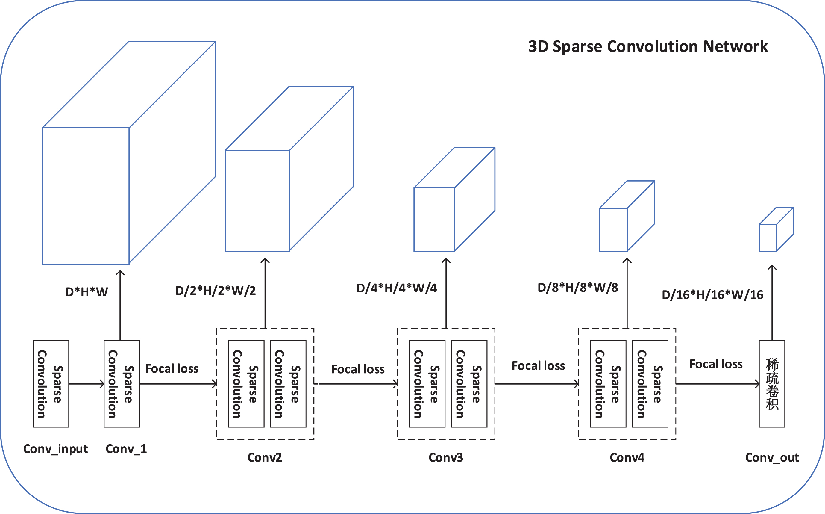
Structure of VoxelBackBone8x Focal.

4 Point cloud object detection

4.1 Dataset

To evaluate the effectiveness of the model in object detection, experiments were conducted on the KITTI open-source dataset for 3D point cloud object detection. The KITTI dataset comprises urban street scenes. During the training process, a total of 7481 frames of data, including point cloud data, image data, and annotation information, were used to train the object detection model. During the testing phase, 7518 frames of point cloud data were employed to perform object detection with the trained model, thus assessing its performance.

Details of experimental equipment: In order to verify the effect of the proposed 3D point cloud object detection model in object detection tasks, the simulation experiment uses KITTI dataset for training and testing in Ubuntu 20.04, Python 3.7, Pytorch 1.12.1, torchvision 0.13.1, CUDA11.3 environments. The hardware parameters of the computer and configuration environment used are processor Inter (R) Xeon (R) W-1270P CPU @3.80G Hz, RAM is 64G. NVIDIA GeForce RTX 3090 video card chip has a memory capacity of 24G.

4.2 Experiment

In this study, the model was trained, tested, and validated on the KITTI dataset. After undergoing 80 rounds of training, the model’s performance was evaluated on the test set using Average Precision (AP) as the primary metric to assess accuracy.

4.2.1 Model comparison

Tables 1 and 2 present the accuracy of our method compared to previous mainstream methods and recent classification models on the KITTI dataset. The object detection task encompasses three primary categories: cars, pedestrians, and bicycles, evaluated across 3D scales. Additionally, different detection difficulties were configured for each detection category. Detection metrics include accuracy for the three detection categories under easy difficulty (IoU = 0.25), moderate difficulty (IoU = 0.5), and hard difficulty (IoU = 0.7).

Table 1
Accuracy comparison between the proposed model and other models on test

Methods Stages Car 3D AP Ped 3D AP Cyclist 3D AP

Easy Mod Hard Easy Mod Hard Easy Mod Hard

PointPillars One 79.1 75.0 68.3 52.1 43.5 41.5 75.8 59.1 52.9

Second One 83.1 73.7 66.2 51.1 42.6 37.3 70.5 53.9 46.9

Part-A2-Net Two 86.0 77.9 72.0 67.7 48.6 44.3 78.6 62.7 57.7

PointRCNN Two 85.9 75.8 68.3 49.4 41.8 38.6 73.9 59.6 53.6

VoxelRCNN Two 90.9 81.6 77.1 – – – – – –

VoxelNet Two 77.5 65.1 57.7 39.5 33.7 31.5 61.2 48.4 44.4

PVRCNN++ Two 79.1 72.6 66.2 53.8 45.2 40.6 73.5 49.5 47.6

Ours Two 79.5 72.9 66.3 54.7 46.4 41.7 76.7 60.8 53.0

Methods	Stages	Car 3D AP	Ped 3D AP	Cyclist 3D AP
PointPillars	One	79.1	75.0	68.3	52.1	43.5	41.5	75.8	59.1	52.9
Second	One	83.1	73.7	66.2	51.1	42.6	37.3	70.5	53.9	46.9
Part-A2-Net	Two	86.0	77.9	72.0	67.7	48.6	44.3	78.6	62.7	57.7
PointRCNN	Two	85.9	75.8	68.3	49.4	41.8	38.6	73.9	59.6	53.6
VoxelRCNN	Two	90.9	81.6	77.1	–	–	–	–	–	–
VoxelNet	Two	77.5	65.1	57.7	39.5	33.7	31.5	61.2	48.4	44.4
PVRCNN++	Two	79.1	72.6	66.2	53.8	45.2	40.6	73.5	49.5	47.6
Ours	Two	79.5	72.9	66.3	54.7	46.4	41.7	76.7	60.8	53.0

Table 2

Accuracy comparison between the proposed model and other models on val

Methods	Stages	Car 3D AP			Ped 3D AP			Cyclist 3D AP
		Easy	Mod	Hard	Easy	Mod	Hard	Easy	Mod	Hard
PointPillars	One	90.8	89.7	81.4	68.8	50.5	45.4	75.6	73.2	65.5
Second	One	90.8	89.7	81.5	71.7	52.4	46.2	74.6	70.3	63.1
Second_iou	One	90.9	89.6	82.1	71.6	56.1	45.3	75.9	74.4	64.3
Part-A2-Net	Two	92.2	89.2	82.6	73.8	60.4	54.6	76.9	75.8	65.4
PointRCNN_iou	Two	96.3	89.4	81.8	70.9	58.6	51.3	79.1	75.0	66.9
PointRCNN	Two	90.7	89.7	81.9	71.3	55.8	48.7	88.5	74.7	65.6
VoxelRCNN	Two	92.1	89.5	84.0	–	–	–	–	–	–
PVRCNN++	Two	95.6	89.2	82.3	69.1	56.2	50.5	75.3	72.9	64.1
Ours	Two	95.9	89.3	82.4	71.1	56.2	48.1	78.5	76.6	69.3

The loss curve during the training process of our model is depicted in Fig. 4. Training loss chart.

Fig. 4

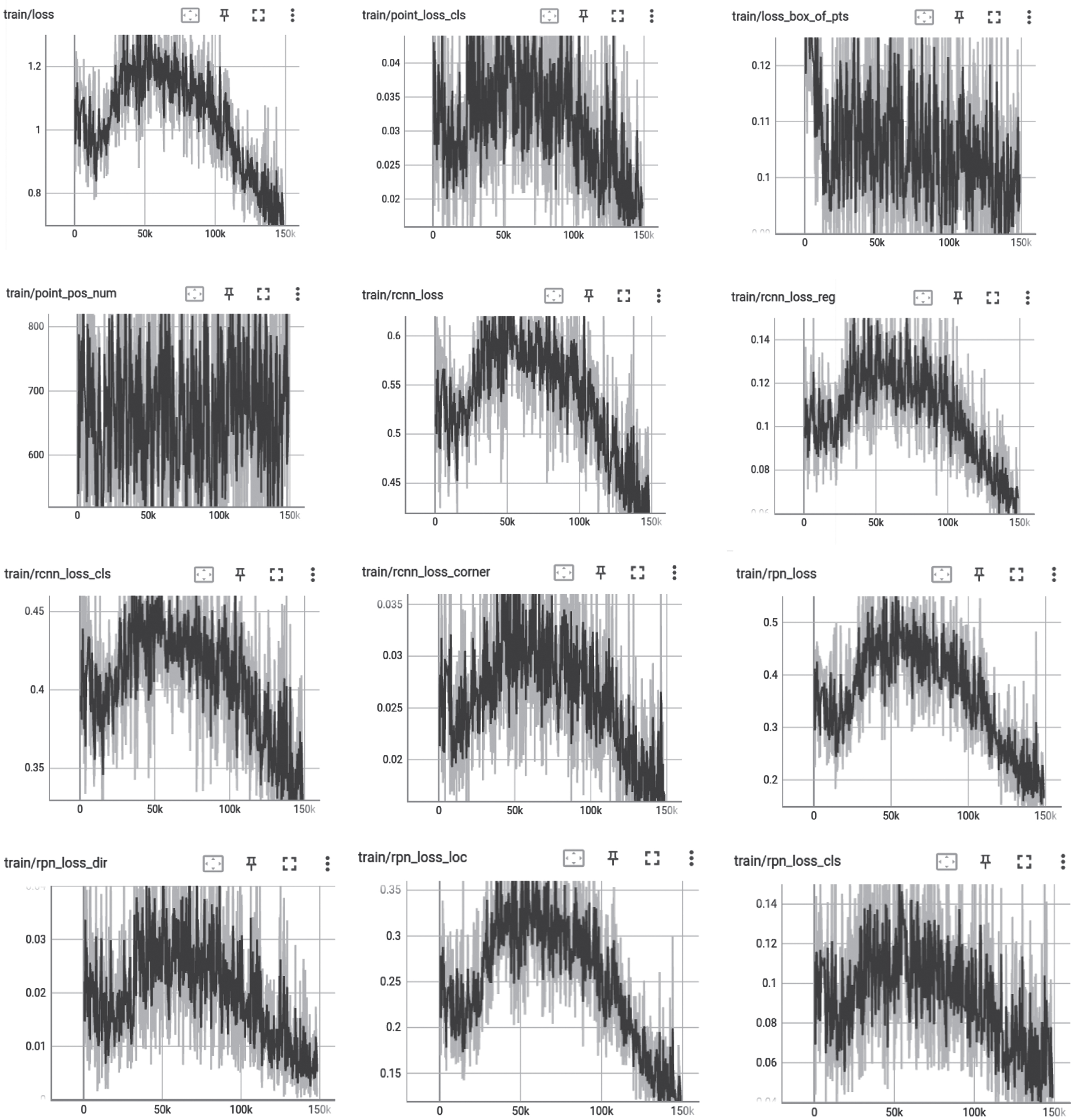
Training loss chart.

4.2.2 FPS experiment

We conducted FPS experiments on our model. Sec_per_example is a time measurement metric that represents the average processing time per sample, indicating the model’s runtime speed. Average predicted number of objects is a metric in the context of object detection tasks, which denotes the average number of predicted objects by the model in each sample.

Table 3
FPS experiment

Models Sec_per_ Average predicted number

example (s) of objections (3769)

PointPillars 0.0238 16.965

Second 0.0283 14.227

Second_iou 0.0300 14.204

Part-A2-Net 0.0531 11.202

PointRCNN_iou 0.0472 7.199

PointRCNN 0.0544 5.706

VoxelRCNN 0.0398 6.027

PVRCNN++ 0.0635 9.240

Ours 0.1347 10.408

Models	Sec_per_	Average predicted number
PointPillars	0.0238	16.965
Second	0.0283	14.227
Second_iou	0.0300	14.204
Part-A2-Net	0.0531	11.202
PointRCNN_iou	0.0472	7.199
PointRCNN	0.0544	5.706
VoxelRCNN	0.0398	6.027
PVRCNN++	0.0635	9.240
Ours	0.1347	10.408

4.2.3 Ablation experiment

We conducted ablation experiments to verify the effectiveness of the proposed modules. Two baseline models were selected as the main subjects for ablation experiments. The improved modules were separately evaluated on the single-stage model “Second” and the two-stage model PVRCNN++ using the validation dataset to compare the detection accuracy. Comparing with the two baseline models, “Second” and PVRCNN++, as shown in Table 4 Ablation experiment.

Table 4
Ablation experiment

Methods Modules Car 3D AP Ped 3D AP Cyclist 3D AP

Voxel BackBone Mean Max Easy Mod Hard Easy Mod Hard Easy Mod Hard

8x Focal MLP VFE

Second √ 90.7 89.6 80.8 70.0 49.5 42.7 74.1 67.6 60.2

√ 95.9 89.5 81.4 68.8 50.1 43.3 75.6 73.2 65.0

PVRCNN √ 95.8 89.3 82.2 68.4 52.0 47.1 76.2 74.5 68.2

++ √ 94.9 89.3 82.5 68.7 52.7 45.3 72.8 71.6 64.5

Methods	Modules	Car 3D AP	Ped 3D AP	Cyclist 3D AP
Second	√		90.7	89.6	80.8	70.0	49.5	42.7	74.1	67.6	60.2
		√	95.9	89.5	81.4	68.8	50.1	43.3	75.6	73.2	65.0
PVRCNN	√		95.8	89.3	82.2	68.4	52.0	47.1	76.2	74.5	68.2
++		√	94.9	89.3	82.5	68.7	52.7	45.3	72.8	71.6	64.5

We performed ablation experiments on the module in addition to experiments on time, rate of detecting samples per second, and average number of predicted objects.

4.2.4 Number of model parameters

4.2.5 Recall experiment

We conducted a comparison of recall rates for our model. Recall rate refers to the proportion of correctly detected samples by the model among all true positive samples. In object detection, positive samples typically refer to the actual existing objects. The formula for calculating recall rate is:

Recall Rate = Number of Correctly Detected Positive Samples / Total Number of Positive Samples.

4.2.6 Visualization results

As shown in Fig. 5. Visualization results, we present partial visual results of our model compared to the baseline model PVRCNN++. Figures (a)–(f) show the visualizations of the model for three frames of point cloud detection in the KITTI dataset, respectively, where Figures (a) and (d), Figures (b) and (e), Figures (c) and (f) are for the same frame of data. Figures (a), (b), and (c) represent visual results of our model, while (d), (e), and (f) show visual results of the baseline model. In the images, objects detected in green are labeled as vehicles, while objects detected in blue are small objects corresponding to pedestrians and bicycles.

Fig. 5

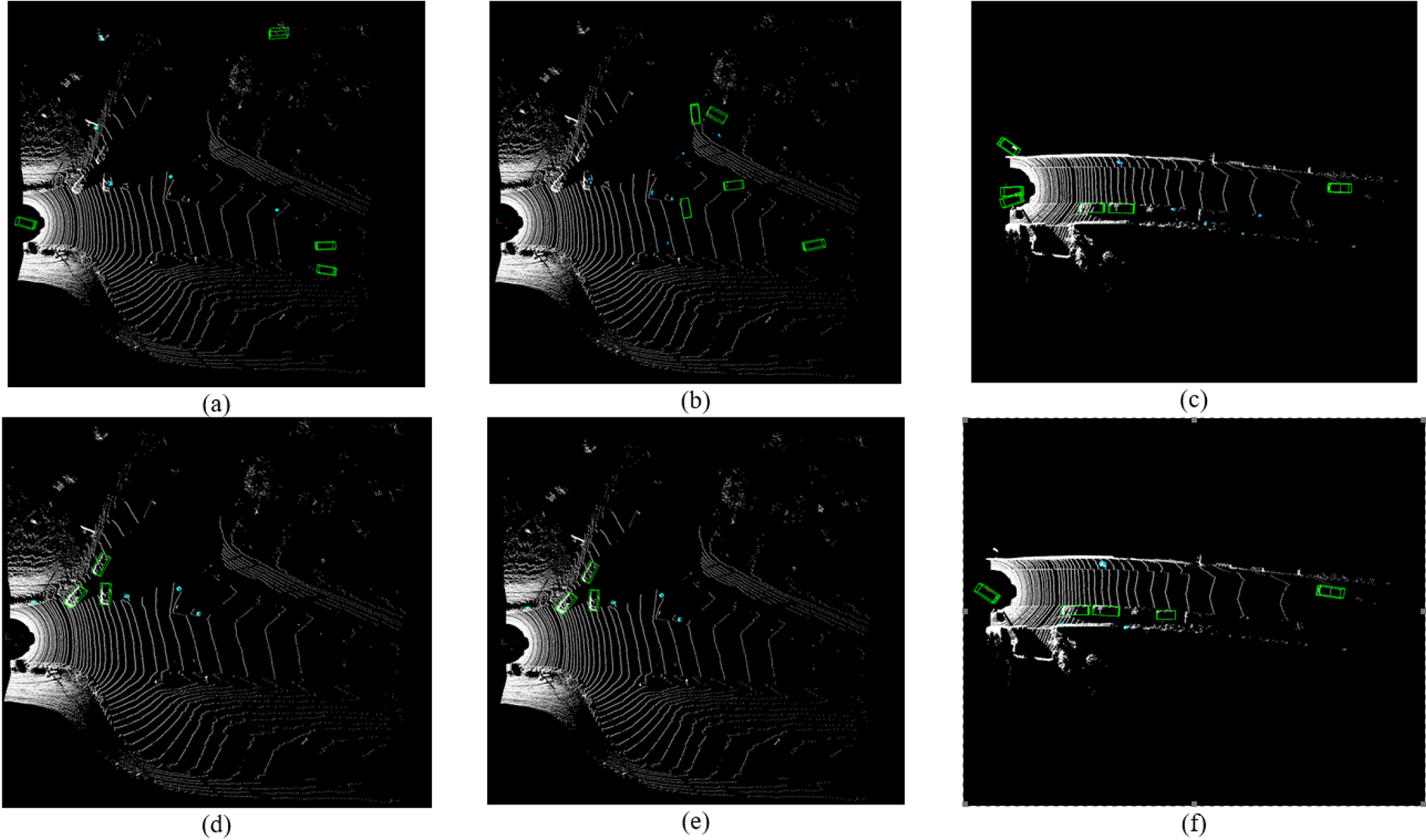
Visualization results.

4.3 Results and discussions

Through comparative experiments on the test dataset in Table 1, our model performs well at all difficulty levels, with values ranging from 66.3% to 79.5%. This shows that the model is able to accurately detect cars in a variety of scenarios, including challenging ones. Performance for pedestrians is relatively low, with values ranging from 41.7% to 54.7%, but slightly better than the other comparison models. This suggests that the model is relatively poor at detecting pedestrians, especially in more challenging situations. The model performs well at detecting cyclists, with values ranging from 53.0% to 76.7%. This shows that the model has a strong ability to identify cyclists in different situations. In addition, our method exhibits a 0.4% improvement in the car detection category compared to the PVRCNN++ model. However, when compared to other two-stage object detection algorithms, it falls slightly short. Nevertheless, in the small target categories of pedestrians and bicycles, our method achieves an accuracy increase of 1.1% and 3.2%, respectively, compared to the PVRCNN++ model, and the improvement is more pronounced compared to other comparative models.

In comparative experiments on the validation dataset in Table 2, our method shows a significant enhancement in the detection accuracy of small targets compared to other comparative methods.

In Fig. 4. Training loss chart, train_loss represents the overall loss throughout the training, measuring the model’s performance on the entire training dataset. point_loss_cls assesses the model’s classification performance on objects within the point cloud, indicating whether the model can correctly identify the object categories in the point cloud. rcnn_loss encompasses the overall loss for the RCNN component, which may include classification loss and regression loss. rcnn_loss_reg evaluates the model’s performance in the task of regressing object bounding boxes, i.e., whether the model can accurately predict the object’s location. rcnn_loss_cls gauges the model’s performance in the task of object classification, assessing whether the model can correctly classify the detected objects. rpn_loss_cls measures the model’s classification performance when generating candidate boxes, indicating whether the model can correctly classify the candidate boxes.

In Table 3, PointPillars and Second have shorter inference times (0.02 seconds), but PointPillars has a higher average number of predicted targets (16.965) and Second has a smaller average number of predicted targets (14.227). Our model has a long inference time (0.1347 seconds) and a moderate average number of predicted targets (10.408). The results indicate that our model exhibits slower detection speeds, significantly higher than most other models. When processing individual samples, our model’s inference speed is relatively slow. In terms of the average predicted number of objects, our model falls within the moderate range compared to other models. This suggests that our model can generate a reasonable number of object detection results in object detection tasks. Regarding the model’s efficiency, from a comprehensive perspective considering both performance and speed, our model’s performance may be relatively lower. Although it can produce a certain number of object detection results, it handles fewer samples per unit of time and operates at a slower pace. This might not be suitable for real-time performance requirements in certain application scenarios.

Tables 4 and 5 show the ablation experiments of the model and the module efficiency experiments.

Table 5
Experiments on time, speed of sample detection per second, and average number of predicted objects

Methods Modules Sec_per_example Average predicted number Time

Voxel BackBone Mean MaxMLP of objections(3769)

8x Focal VFE

Second √ 0.0336 13.812 10.5h

√ 0.0302 13.850 6.3h

PVRCNN ++ √ 0.1315 9.768 18.8h

√ 0.0624 11.247 10.8h

Methods	Modules	Sec_per_example	Average predicted number	Time
Second	√		0.0336	13.812	10.5h
		√	0.0302	13.850	6.3h
PVRCNN ++	√		0.1315	9.768	18.8h
		√	0.0624	11.247	10.8h

VoxelBackBone8x Focal: Building upon the Mean Max MLP VFE module, the 3D backbone network was replaced with VoxelBackBone8x for feature extraction. Experimental results on the validation dataset indicated that, in comparison to the baseline model, in single-stage object detection, the average detection accuracy for cars decreased by 2%, while that for pedestrians and small objects such as bicycles decreased by 2.7% and 1.9%, respectively. In two-stage object detection, the average detection accuracy for cars decreased by 0.2%, and for pedestrians and small objects like bicycles, it decreased by 2.2% and 5.2%, respectively. These results suggest that the VoxelBackBone8x Focal module can enhance the model’s sensitivity to small objects to some extent.

Mean Max MLP VFE: In the scenario where the 3D backbone network remains unchanged, the voxel encoding module was replaced with Mean VFE. Experimental results on the validation dataset showed that, in single-stage object detection, compared to the baseline model, the average accuracy for car detection decreased by 0.3%, while that for pedestrians and small objects such as bicycles decreased by 2.6% and 2%, respectively. In two-stage object detection, the average accuracy for car detection decreased by 0.1% compared to the comparison model, whereas for pedestrians and small objects like bicycles, it decreased by 8.9% and 2.2%, respectively. These results suggest that the Mean Max MLP VFE module can, to some extent, expand the feature representation of the input model.

When only the VoxelBackBone8x Focal module is present, the single-stage model exhibits shorter detection times, a higher average predicted sample count, and overall superior speed compared to the two-stage model. Experimental results indicate that the VoxelBackBone8x Focal module performs more efficiently in the single-stage model, resulting in faster detection speeds and a greater number of predicted samples.

When only the Mean MaxMLP VFE module is used, the single-stage model still maintains shorter detection times. Both models exhibit similar average sample prediction counts and samples detected per second, but the single-stage model remains superior to the two-stage model. Experimental results demonstrate that the Mean MaxMLP VFE module exhibits certain advantages in the single-stage model, and even within the two-stage model, it maintains relatively higher speeds.

These two experimental observations indicate that the single-stage model performs better in terms of speed, regardless of whether the VoxelBackBone8x Focal module or the Mean MaxMLP VFE module is used. This may be attributed to the fact that single-stage models are generally more suitable for applications requiring efficient object detection, as they are more compact and directly perform detection tasks, whereas two-stage models require additional steps for detection and recognition, which may result in some performance loss.

In Table 6, Compared with PointPillars and Second, the model of Part-A2-Net is larger. The number of our model parameters is 160.32 million, which has the largest parameter size among all listed models except Part-A2-Net.Although our model has more parameters compared to other models, approaching or even surpassing some complex models, this indirectly reflects that our model also possesses a larger capacity to accommodate more feature information, exhibiting stronger fitting and expressive capabilities, with the potential to capture more complex features and patterns. It is expected to deliver better performance in future deployment stages.

Table 6

Model parameter quantity

Methods	Params(M)
PointPillars	19.38
Second	21.36
Part-A2-Net	255.36
PointRCNN_iou	16.29
PointRCNN	16.29
VoxelRCNN	30.42
PVRCNN++	52.57
Ours	160.32

In Table 7, we evaluated the model comprehensively using different recall rate metrics. At an IoU threshold of 0.3, our model’s Recall Rate is moderate compared to other models, with no significant performance advantage or disadvantage. At an IoU threshold of 0.5, the Recall Rate of our model is also moderate, similar to the performance of other models. At an IoU threshold of 0.7, the Recall Rate of our model similarly falls within the moderate range, with no significant performance advantage.

Table 7

Recall rate experiment

Methods	Recall_0.3		Recall_0.5		Recall_0.7
	roi	rcnn	Roi	rcnn	roi	rcnn
PointPillars	–	0.94	–	0.88	–	0.64
Second	–	0.95	–	0.89	–	0.67
Second_iou	0.97	0.97	0.93	0.93	0.71	0.71
Part-A2-Net	0.97	0.97	0.93	0.94	0.71	0.75
PointRCNN_iou	0.90	0.90	0.87	0.88	0.69	0.74
PointRCNN	0.90	0.90	0.87	0.87	0.69	0.74
VoxelRCNN	0.98	0.98	0.97	0.97	0.83	0.87
PVRCNN++	0.97	0.97	0.93	0.93	0.72	0.76
Ours	0.90	0.90	0.87	0.87	0.69	0.74

In terms of detection of small objects, the number of detections of our model is significantly higher compared to the number of detections of the benchmark model, which indicates that our model is largely more sensitive to the detection of small objects and is able to capture more small targets. In terms of detecting large objects in cars, the number of detections of our model is roughly the same as that of the benchmark model, which also indicates that our model is at the same level as the mainstream model in detecting large objects.

5 Conclusion

We propose a sparse point cloud object detection method based on adaptive voxel coding and focal sparse convolution, which can better improve the detection accuracy of small objects in the detection model. We found that by expanding the extraction of features and increasing the calculation of focal loss, the missing sparse small object detection can be compensated to a large extent. In the voxel encoding stage, we employ an adaptive pooling combination strategy along with multi-layer perceptrons and fully connected operations to expand the input features of the point cloud. Furthermore, in the 3D backbone network stage, we utilize custom sparse convolution operations to enable the backbone network to better adapt to different feature data. Additionally, by introducing multiple layers of Focal Loss, we address the issue of imbalanced detection categories, enabling the model to focus more on sparse and smaller objects. Experimental results on the KITTI public dataset demonstrate that in pedestrian and bicycle detection tasks, compared to the PVRCNN++ model, our method achieves a 1% and 2.1% improvement in detection accuracy for pedestrians and bicycles, respectively, outperforming other compared detection algorithms. This fully validates the effectiveness of the proposed improvement in point cloud object detection.

Through iterative experiments, this paper provides several insights: to make full use of point cloud data, it is crucial to enhance the richness of point cloud features during input feature processing. Additionally, in the feature extraction stage, attention should be given not only to dense point cloud features but also to sparse small targets. It’s important to note that this study only focuses on three-dimensional point cloud object detection tasks, and the robustness of the detection model and real-time detection speed for deployment in actual vehicles have not been evaluated. Future work may involve deploying the model on real vehicles for practical applications.

Footnotes

Acknowledgments

This work was supported in part by the Scientific research start-up project of Shanghai Institute of Technology under Grant No. YJ2022-40; in part by the collaborative innovation fund of Shanghai Institute of Technology under Grant.

Declarations

There is no conflict of interest in this paper, and the data set used in the experiment is public and no confidential.

References

Cooper: Cooperative Perception for Connected Autonomous Vehicles Based on 3D Point Clouds

, Li

and Liu

, Research on 3D Point Cloud Object Detection Methods Based on Deep Learning[C]//2023 2nd International Conference on Big Data, Information and Computer Network (BDICN).IEEE, (2023), 34–37.

Guo

, Wang

, Hu

, et al., Deep learning for 3d point clouds: A survey[J], IEEE Transactions on Pattern Analysis and Machine Intelligence 43(12) (2020), 4338–4364.

Huang

, Wang

and Li

, Research overview on 3D object detection methods[J], Journal of Intelligent Science and Technology 5(1) (2023), 7–31.

Guo Yifeng, , Wu Dihao , Wei Qingmin, , A Comprehensive Overview of Deep Learning-Based 3D Object Detection Methods for Point Clouds[J], Application Research of Computers / Jisuanji Yingyong Yanjiu 40(1) (2023).

Ji Yimu, , Chen Zhiyu, , Tian Penghao, , et al., A Review of 3D Object Detection Methods in Unmanned Driving[J], Journal of Nanjing University of Posts and Telecommunications: Natural Science Edition 39(4) (2019), 72–79.

Zhang

, Wang

, Zhao

, et al., U-Select RCNN: An Effective Voxel-based 3D Object Detection Method with Feature Selection Strategy[C]//2022 34th Chinese Control and Decision Conference (CCDC). IEEE, (2022), 3581–3586.

Tao

and Su

, Research on object detection algorithm of 3D point cloud PointPillar based on attention mechanism[C]//2022 China Automation Congress (CAC), IEEE, (2022), 4382–4385.

Lang

A.H.

, Vora

, Caesar

, et al., Pointpillars: Fast encoders for object detection from point clouds[C]//Proceedings of the IEEE/CVF conference on computer vision and pattern recognition, (2019), 12697–12705.

10.

Yan

, Mao

and Li

, Second: Sparsely embedded convolutional detection[J], Sensors 18(10) (2018), 3337.

11.

Zhou

and Tuzel

, Voxelnet: End-to-end learning for point cloud based 3d object detection[C]//Proceedings of the IEEE conference on computer vision and pattern recognition, (2018), 4490–4499.

12.

Yin

, Zhou

and Krahenbuhl

, Center-based 3d object detection and tracking[C]//Proceedings of the IEEE/CVF conference on computer vision and pattern recognition, (2021), 11784–11793.

13.

Wei

, Wang

, Fan

, et al., An Efficient Point Cloud-based 3D Single Stage Object Detector[C]//5th CAA International Conference on Vehicular Control and Intelligence (CVCI). IEEE, (2021), 1–5.

14.

Yang

, Luo

and Urtasun

, Pixor: Real-time 3d object detection from point clouds[C]//Proceedings of the IEEE conference on Computer Vision and Pattern Recognition, (2018), 7652–7660.

15.

Shi

, Wang

and Li

, Pointrcnn: 3d object proposal generation and detection from point cloud[C]//Proceedings of the IEEE/CVF conference on computer vision and pattern recognition, (2019), 770–779.

16.

Chen

, Liu

, Shen

, et al., Fast point r-cnn[C]//Proceedings of the IEEE/CVF international conference on computer vision, (2019), 9775–9784.

17.

, Wang

and Wang

, Lidar r-cnn: An efficient and universal 3d object detector[C]//Proceedings of the IEEE/CVF Conference on Computer Vision and Pattern Recognition, (2021), 7546–7555.

18.

C.R.

, Yi

, Su

, et al., Pointnet++: Deep hierarchical feature learning on point sets in a metric space[J], Advances in Neural Information Processing Systems (2017), 30.

19.

Yuan

, Wang

, Liu

, et al., A Rail Detection Method Using Bird’s Eye View of LiDAR Point Clouds[C]//2023 6th International Conference on Electronics Technology (ICET). IEEE, (2023), 120–126.

20.

Yang

, Sun

, Liu

, et al., 3dssd: Point-based 3d single stage object detector[C]//Proceedings of the IEEE/CVF conference on computer vision and pattern recognition, (2020), 11040–11048.

21.

Shi

, Guo

, Jiang

, et al., Pv-rcnn: Point-voxel feature set abstraction for 3d object detection[C]//Proceedings of the IEEE/CVF conference on computer vision and pattern recognition, (2020), 10529–10538.

22.

Shi

, Jiang

, Deng

, et al., PV-RCNN++: Point-voxel feature set abstraction with local vector representation for 3D object detection[J], International Journal of Computer Vision 131(2) (2023), 531–551.

23.

Mao

, Xue

, Niu

, et al., Voxel transformer for 3d object detection[C]//Proceedings of the IEEE/CVF International Conference on Computer Vision, (2021), 3164–3173.

24.

Cui

and Zhang

, PVF-NET: Point & Voxel Fusion 3D Object Detection Framework for Point Cloud, 2020 17th Conference on Computer and Robot Vision (CRV), Ottawa, ON, Canada, (2020), 125–133.

25.

Luo

, Zhou

, Tao

, et al., Dynamic multitarget detection algorithm of voxel point cloud fusion based on PointRCNN[J], IEEE Transactions on Intelligent Transportation Systems 23(11) (2022), 20707–20720.