Heating load prediction in buildings using decision tree machine learning method

Abstract

In recent years, the burgeoning imperative of energy-efficient building management practices has surged dramatically, underscoring an urgent mandate for comprehensive studies that integrate cutting-edge optimization algorithms with precise heating load forecasting techniques. These studies are not merely endeavors; they represent concerted efforts to increase building energy efficiency and address mounting concerns regarding sustainability and resource utilization. In the intricate domain of heating, ventilation, and air conditioning (HVAC) systems, energy optimization challenges are being meticulously confronted through rigorous exploration and the application of innovative problem-solving methodologies. This pioneering study introduces groundbreaking methodologies by seamlessly integrating two state-of-the-art optimization algorithms— the Red Fox Optimization and the Golden Eagle Optimizer— with the Decision Tree model. This fusion is aimed at enhancing the accuracy of heating load predictions and streamlining HVAC system optimization processes, marking a significant leap toward achieving heightened energy efficiency and operational efficacy in building management practices. The study emphasizes the significance of precise heating load prediction in advancing energy efficiency, realizing cost savings, and fostering environmental sustainability in building management. Furthermore, it delves into the multifaceted impact of various building features on heating load, encompassing variables such as glazing area, orientation, height, relative compactness, roof area, surface area, and wall area. These insights furnish actionable intelligence for refined decision-making processes in both building design and operation. Based on the results, the DT single model experienced the weakest performance among the three models, with R ² = 0.975 and RMSE = 1.608. The model DTFO (DT + FOX) achieves an extraordinary R ² value of 0.996 and RMSE value of 0.961 for heating load prediction, surpassing the performance benchmarks set by other models. This achievement holds considerable promise for aiding engineers in crafting energy-efficient buildings, particularly within the swiftly evolving landscape of smart home technologies.

Keywords

Decision tree heating load red fox optimization golden eagle optimizer

1 Introduction

The construction industry is a significant energy consumer and carbon emitter within contemporary society [1]. Mitigating building energy consumption and its linked carbon emissions calls for the effective prediction of building thermal loads, a vital aspect with extensive utility in optimizing HVAC systems [2], enhancing the operation of thermal energy storage [3], planning energy distribution systems [4], and managing smart grids [5], to name a few. To determine a structure’s cooling load (CL) or heating load (HL), it is essential to scrutinize the temperature profiles within smart homes. When the interplay between building structure and energy needs is understood, architects and builders can formulate energy-efficient building designs that optimally utilize energy for heating and cooling. Therefore, estimating a building’s HL and CL has posed a longstanding challenge in building energy efficiency [6–8]. The prediction of energy consumption holds a significant place in research, considering that it accounts for roughly 30% of the overall energy usage and contributes to approximately 33% of carbon emissions in 2021 [9]. Even with advancements in the construction industry, current initiatives fall short of achieving the 1.5°C scenario, necessitating the implementation of intelligent and sustainable infrastructures to accommodate the swiftly expanding urban landscape. Predicting and modeling energy consumption are essential to developing resource-efficient and intelligent infrastructure. Notably, three primary approaches for modeling and forecasting building energy consumption are physical, data-driven, and hybrid models [10]. Among the methodologies considered, data-driven approaches have become the most apt for integrating into smart homes [11].

In the physical models, predictions are made using equations that describe the physical dynamics of a system. In contrast, data-driven methods use historical system behavior data to generate output. Among data-driven methods, those employing regression models to identify the most precise function for mapping input parameters to observed output can be categorized into statistical and machine-learning methods [12, 13]. In statistical methodologies, the complexity of these functions is frequently preordained by the regression model, where the parameters and architecture of the model are explicitly specified. Conversely, within the domain of machine learning [14, 15], the methodology takes a divergent path as it autonomously adjusts and comprehends the complexity of the functions, typically through iterative processes such as training and optimization [16]. This distinction illuminates the intrinsic adaptability and self-learning prowess inherent in machine learning algorithms, setting them apart from traditional statistical approaches.

Efficiently managing and optimizing building energy consumption necessitates comprehensive data on the building’s performance and environmental conditions. While electricity, gas, and heating supply represent critical energy resources within a structure, the key applications for these resources encompass elevators, heating, ventilation, air conditioning (HVAC), domestic hot water, and more. Notably, among these energy sources, the effective operation of HVAC systems and the provision of indoor environmental conditions stand out as crucial elements in evaluating a building’s energy efficiency [17, 18]. HVAC systems, which serve as fundamental building infrastructure, are responsible for modulating the internal CL and HL of residential structures. While the necessity of these systems in buildings is undeniable, a substantial concern arises from the fact that approximately 40% of all energy consumption, particularly in office buildings, is attributed to these systems [19, 20]. Accurate prediction of thermal loads is a crucial factor in optimizing building heating and cooling expenses. Any deviations from the optimally scheduled load values can significantly escalate the overall operational costs [21]. Within engineering and the context of forecasting HL, the Decision Tree (DT) algorithm is a valuable instrument known for its proficiency in managing intricate relationships within datasets. As SB Kotsiantis highlighted in their foundational DT research [22], these models have proven their effectiveness in capturing intricate interdependencies among diverse parameters. Consequently, engineers benefit from a robust framework, enabling accurate estimations of HL demands across various building scenarios [23].

Researchers have employed various methodologies to forecast heating and cooling loads and energy demand across diverse building contexts [24–31]. For instance, in one study [32], the MLP method was utilized with meteorological data to predict building heating loads, while another [33] simultaneously forecasted both cooling and heating loads using meteorological and date data inputs. Furthermore, a study [34] investigated a building’s energy performance employing machine learning techniques such as general linear regression, artificial neural networks, decision trees, support vector regression (SVR), and ensemble inference models for cooling and heating load forecasting. The impact of structural and interior design factors on cooling loads was explored through a range of regression models [35], while HVAC system energy demand was estimated from cooling and heating load requirements using various regression models. In commercial buildings, cooling load and electric demand were forecasted for short-term and ultrashort-term management [36], augmenting energy efficiency through a hybrid SVR approach. Additionally, the SVR method was applied [37] to project cooling loads in a large coastal office building in China, introducing a novel vector-based SVR model to enhance robustness and forecasting precision [31].

This research primarily aims to offer indispensable support to architects and design engineers in the pre-design phase of energy-efficient building projects, focusing specifically on the precise estimation of HL. The DT model has been meticulously developed to realize this objective as a robust tool for accurately predicting building energy loads. This predictive capacity holds remarkable significance within this context. The model’s performance has been further enhanced by employing two distinct optimization algorithms: the Fox Optimization (FOX) optimizer and the Golden Eagle Optimizer (GEO). The outcomes generated by these three models, comprising a single model and two optimized versions, underwent rigorous assessment involving a range of performance metrics, such as R², RMSE, MAE, SI, and n10-index. Consequently, this extensive evaluation identified the superior ensemble model, essential for precisely forecasting HLs in building systems.

The paper’s subsequent sections follow a structured progression: Section 2 meticulously delineates the materials and methodologies harnessed in the study, offering transparency into the research process. Section 3 unfolds the paper’s core, unveiling the research findings and initiating comprehensive discussions that probe their significance and implications. Finally, Section 4 concludes the paper, summarizing key takeaways and their broader implications to opt for the best-performed model to use in designing energy-efficient buildings.

2 Materials and methods

2.1 Data collection

This research aims to predict building HL using experimental energy consumption data. The study employs a DT simulation approach with two specialized optimizers to refine DT hyperparameters. Input parameters, such as relative compactness, surface area, wall area, and more, are used to estimate HL in kilowatts (kW), and Table 1 summarizes the input and output parameter statistics [38, 39].

Table 1
The statistical properties of the input variable of heating

Variables Indicators

Category Min Max Avg St . Dev .

RelativeCompactness Input 0.62 0.98 0.764 0.106

SurfaceArea Input 514.5 808.5 671.7 88.09

WallArea Input 245 416.5 318.5 43.63

RoofArea Input 110.3 220.5 176.6 45.17

Overall, Height Input 3.5 7 5.25 1.751

Orientation Input 2 5 3.5 1.119

GlazingArea Input 0 0.4 0.234 0.133

GlazingAreaDistribution Input 0 5 2.813 1.551

Heating Output 6.01 43.1 22.31 10.09

Variables	Indicators
RelativeCompactness	Input	0.62	0.98	0.764	0.106
SurfaceArea	Input	514.5	808.5	671.7	88.09
WallArea	Input	245	416.5	318.5	43.63
RoofArea	Input	110.3	220.5	176.6	45.17
Overall, Height	Input	3.5	7	5.25	1.751
Orientation	Input	2	5	3.5	1.119
GlazingArea	Input	0	0.4	0.234	0.133
GlazingAreaDistribution	Input	0	5	2.813	1.551
Heating	Output	6.01	43.1	22.31	10.09

2.2 Overview of machine learning model

2.2.1 Decision Tree (DT)

The DT is a supervised learning approach for regression and classification tasks [40]. It involves a hierarchical tree structure with distinct levels or divisions. In regression tasks, where no specific category or class is defined, this technique makes predictions based on independent variables [41, 42].

The model illustrated in Fig. 1 represents a straightforward DT. It consists of a single binary target variable, Y (0or1), and two continuous variables, x1 and x2, with values ranging from 0 to 1. This structure can be visualized as a partitioned physical space, as shown in Fig. 2. Segmenting the sample space into discrete, non-overlapping, and exhaustive segments is a fundamental aspect of this analytical framework. Each segment corresponds directly to a unique leaf node, the final output resulting from a sequence of decision-making steps. Each data point is assigned to a single segment, a leaf node. DT analysis aims to identify the optimal model for effectively partitioning the available data into discrete segments.

Fig. 1

Sample DT based on binary target variable Y.

Fig. 2

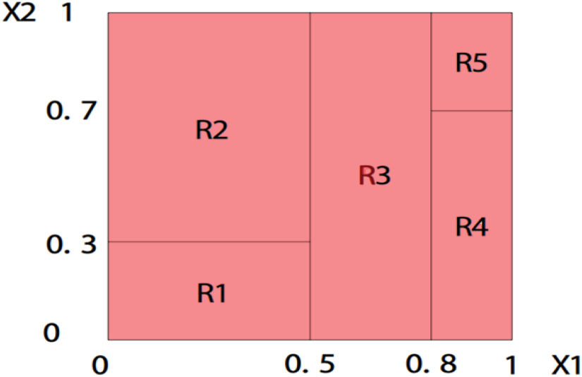
DT illustrated using a sample space view.

A DT model is primarily composed of nodes and branches. The key phases in constructing such a model involve the processes of splitting, stopping, and pruning.

2.3 Overview of optimization algorithms

2.3.1 Red Fox Optimization (FO)

The Red Fox Optimization Algorithm (RFOA) is inspired by red fox hunting behavior and consists of two main stages: exploitation and exploration. The exploitation stage mirrors a fox closing in on its prey, while their relative distance influences the exploration phase. The algorithm operates with a constant population of foxes, as outlined below [43]:

\bar{x} = (x_{0}, x_{1}, \dots, x_{n - 1})

(1)

To identify each fox, denoted as ${\bar{x}}^{t}$ in iteration t, the notation ${({\bar{x}}_{j}^{i})}^{t}$ is introduced. Here, i represents the number of foxes, and j corresponds to the coordinates within the solution space, determined by the dimensions.

The notation ${(\bar{x})}^{(i)} = [{(x_{0})}^{(i)}, {(x_{1})}^{(i)}, {(x_{2})}^{(i)}, \dots, {(x_{n - 1})}^{(i)}]$ is used to represent each point within the solution space 〈a, b 〉 ⁿ, where $a, b \in ℝ$ .

Additionally, concerning the solution space, a function $f \in ℝ^{n}$ considered as the typical n-variable function. Should the function’s value be, $f ({(\bar{x})}^{(i)})$ , corresponds to a global maximum or minimum within the interval 〈a, b〉, then $({(\bar{x})}^{(i)})$ is considered to be the optimal solution.

When the foxes cannot locate prey, family members venture out in search of food. When they discover a more favorable area, they share the location, and the population is sustained based on the associated cost. The Euclidean squared distance serves as the metric for this purpose:

D ({({\bar{x}}^{i})}^{t}, {({\bar{x}}^{b})}^{t}) = \sqrt{{({\bar{x}}^{i})}^{t} - {({\bar{x}}^{b})}^{t}},

(2)

Here $({\bar{x}}^{b})$ signifies $({\bar{x}}^{best})$ , and the individuals within the population shift their positions in the direction of the best performer:

{({\bar{x}}^{i})}^{t} = {({\bar{x}}^{i})}^{t} + α * S * ({({\bar{x}}^{b})}^{t} - {({\bar{x}}^{i})}^{t}),

(3)

In this case, α is randomly selected from the range $(0, d ({({\bar{x}}^{i})}^{t}, {({\bar{x}}^{b})}^{t}))$ , and ‘S’ denotes the ‘sign’ word.

The random value β, falling within the range <0,1>, is applied as a single setting for all individuals within the population. This value characterizes the action of the fox as: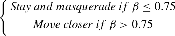

{\begin{matrix} Stay and masquerade if β ⩽ 0.75 \\ Move closer if β > 0.75 \end{matrix}

A sophisticated Cochleoid formula represents the actions of individuals if β affects the population’s migration in a certain cycle. The fox radius has two components: φ₀∈ 〈 0, 2π 〉 for the initial observation angle and α∈ 〈 0, 0.2 〉as a scaling parameter, preset for all individuals in the population to represent random changes in distance as the fox approaches the victim:

r = {\begin{matrix} a \frac{\sin φ_{0}}{φ_{0}} if φ_{0} \neq 0 \\ δ if φ_{0} = 0 \end{matrix}

(4)

Here, δ is a randomly determined variable that depends on the weather and is set once at the beginning of the process. It ranges from 0 to 1. The following is a description of the population’s movement pattern:

{\begin{matrix} x_{0}^{new} = ar * cos (φ_{1}) + x_{0}^{ac} \\ x_{1}^{new} = ar * sin (φ_{1}) + ar * cos (φ_{2}) + x_{1}^{ac} \\ x_{2}^{new} = ar * sin (φ_{1}) + ar * sin (φ_{2}) + ar * cos (φ_{3}) + x_{2}^{ac} \\ \dots \\ x_{n - 2}^{new} = ar * \sum_{q = 1}^{n - 2} sin (φ_{q}) + ar * cos (φ_{n - 1}) + x_{n - 2}^{ac} \\ x_{n - 1}^{new} = ar * sin (φ_{1}) + ar * cos (φ_{2}) + \dots + ar * sin (φ_{n - 1}) + x_{n - 1}^{ac} \end{matrix}

(5)

Where “ac” in $x_{0}^{ac}$ stands for “actual” and φ₁, φ₂, φ₃, and so on, up to φ_n-1, all fall within the range of 〈0, 2π〉.

To simulate this action in every iteration, 5% of the least successful candidates are chosen based on the criterion function. This choice is made as a subjective tendency to bring about little variances among the bunch. Two of the highest-performing people are chosen to create an alpha pair during iteration t:

${({\bar{x}}^{(1)})}^{t} & {({\bar{x}}^{(2)})}^{t}$ , and the habitat’s center is computed using the following equation. The habitat’s extent is determined by the square of the Euclidean distance between the couple respectively:

{(H^{cntr})}^{t} = \frac{{({\bar{x}}^{(1)})}^{t} + {({\bar{x}}^{(2)})}^{t}}{2}

(6)

{(H^{diamtr})}^{t} = \sqrt{{({\bar{x}}^{(1)})}^{t} - {({\bar{x}}^{(2)})}^{t}}

(7)

Here, ‘H’ means habitat. In each iteration, a random parameter q, ranging from 0to 1, is selected to dictate the substitutions made during the repetition as follows:

{\begin{matrix} Reproduction Of The Alpha Couple if q < 0.45 \\ New Nomadic Individual if q ⩾ 0.45 \end{matrix}

(8)

The top two candidates denoted as ${({\bar{x}}^{(1)})}^{t}$ and ${({\bar{x}}^{(2)})}^{t}$ , are merged to create a new candidate represented as ${({\bar{x}}^{(rep)})}^{t}$ , where “rep” signifies reproduction. This combination occurs as follows:

{({\bar{x}}^{(rep)})}^{t} = q \frac{{({\bar{x}}^{(1)})}^{t} + {({\bar{x}}^{(2)})}^{t}}{2}

(9)

RFOA (Red Fox Optimization Algorithm)

1: Commence,

2: Establish the algorithm’s parameters: the fitness functionf (0), the number of iterations T, the initial fox observation angleφ₀, the maximum populationsizen, weather conditionsθ, and the solutionspacerange 〈a, b 〉 ,

3: Create a population of n foxes randomly distributed within the solution space.

4: t = 0

5: whilet ⩽ Tdo

6: Define iteration coefficients: fox proximity change (α), scaling parameter (α) .

7: For every fox within the current population,

8: Organize individuals based on their fitness function values,

9: Select

{({\bar{x}}^{b})}^{t}

10: Compute the repositioning of individuals as per Equation (2) ,

11: If the new position is superior to the previous one, then

12: Relocate the fox to the new position,

13: else

14: Revert the fox to its previous location,

15: end if

16: Determine the parameter β to define the fox’s hunting awareness,

17: If the fox remains unnoticed, then

18: Calculate the fox’s observation radius (r) using Equation (4) ,

19: Compute the repositioning based on Equation (5) ,

20: else

21: The fox maintains its current position to remain concealed,

22: end if

23: end for

24: Arrange the population following the fitness function,

25: Eliminate the poorest –performing foxes from the group, or they fall victim to hunters,

26: Introduce new foxes into the population using Equation (8) as nomadic foxes outside the habitat or through reproduction from the alpha couple withinthe herd, as outlined in Equation (9) .

27: t ++ ,

28: end while

29: Return the fittest fox

{(\bar{x})}^{b},

30: Stop.

2.3.2 Golden Eagle Optimizer (GEO)

The hunting behavior of golden eagles can be mathematically delineated as follows [44]:

•The rotational movement exhibited by golden eagles

The exploration into the spiraling flight patterns of golden eagles revolves around a research inquiry where one eagle, denoted as n, selects its target prey from a different eagle through a random process fand loops the finest prior advert of f, with the ability to encircle its recollection(fin { 1, 2, . . . , PopSize }) .

•Selecting a Target from Potential Victims

During the iterative process, exploration agents adjust their positions by retrieving data from a collective repository, whereas the golden eagles in GEO’s system haphazardly choose prey from the memory of any fellow flock member without being restricted by spatial nearness.

•Attack (exploitation)

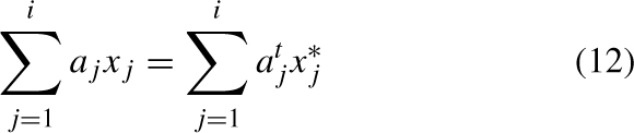
The computation of the attack vector, which extends from the present location of the golden eagle n to its recollected prey, is attainable Equation (10):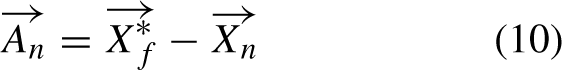

\vec{A_{n}} = \vec{X_{f}^{*}} - \vec{X_{n}}

(10)

Given this situation, $\vec{X_{n}}$ signifies the current place of the eagle n, $\vec{A_{n}}$ denotes the vector of attack utilized by the eagle n, and $\vec{X_{f}^{*}}$ relates to the best position (prey) that the eagle has investigated up to this point f.

•Cruise (exploration)

The cruise vector arises from altering the attack vector along the tangent of the circle in i-dimensional space, which symbolizes the speed of the prey and is established by Equation (11)’s hyperplane equation.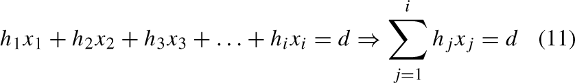

h_{1} x_{1} + h_{2} x_{2} + h_{3} x_{3} + \dots + h_{i} x_{i} = d \Rightarrow \sum_{j = 1}^{i} h_{j} x_{j} = d

(11)

\sum_{j = 1}^{i} a_{j} x_{j} = \sum_{j = 1}^{i} a_{j}^{t} x_{j}^{*}

(12)

Given this situation, 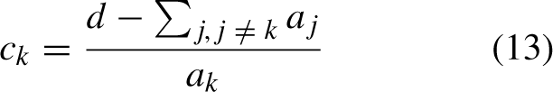$\vec{P} = [p_{1}, p_{2}, p_{3}, \dots, p_{i}]$ stands as a random position situated on the hyperplane, whereas $\vec{H} = [h_{1}, h_{2}, h_{3}, \dots, h_{i}]$ represents the mean vector. The vector of variables is indicated by X = [x₁, x₂, x₃, …, x_i] and d is definite as the dot creation of $\vec{H}$ and $\vec{P}$ , which can alternatively be described as the result of summing the products of h_j and p_j for j reaching from1 to i. Seeing $\vec{X_{n}}$ to symbolize the position of the eagle labeled as n and $\vec{A_{n}}$ by considering it as the mean vector of the hyperplane, the hyperplane association can be determined of ${\vec{C}}_{n}^{t}$ (The cruising vector for the golden eagle n during iteration t) using Equation (12). In this scenario, $X^{*} = [x_{1}^{*}, x_{2}^{*}, x_{3}^{*}, \dots, x_{i}^{*}]$ is characterized as the selected prey’s position, A_n = [a₁, a₂, a₃, …, a_i] symbolizes the assault vector and X = [x₁, x₂, x₃, …, x_i] indicates the variable vector of decisions or designs. After calculating the cruising plane for eagle ‘n’ during iteration t, the subsequent phase involves creating a cruising vector within the same plane. Attaining the ultimate dimension necessitates the fulfillment of the plane equation, yielding a solitary fixed variable and i1 uncorrelated variable. In this process, an arbitrary point ^′C′ in i dimensions is determined on the path plane for golden eagle ‘n’ in the first step. Choose a single parameter from the set i-variable designate a fixed element with index k, distinct from the subset containing zero elements in the attack vector $\vec{A_{n}}$ . A zero coefficient in Equation (11) permits that variable to vary independently along its axis as others change. For instance, in a three-dimensional space as such3x₁ + 2x₂ = 10, ifk = 3, and random standards are allocated to x₁and x₂, like {x₁ = 2, x₂ = 5 } , this leads to a boundless collection of points that meet the criteria of the plane’s equation, similar to { [2, 5, 1] , ] 2, 5, 2] , ] 2, 5, 3] , … } . During Step 2, allocate values to all variables excluding the k - th one, and in Step 3, ascertain the k - th variable’s value with the aid of Equation (13):

c_{k} = \frac{d - \sum_{j, j \neq k} a_{j}}{a_{k}}

(13)

In this structure, c_k represents the k - th component of point C, a_j representing the j - th component in the attack vector A_n, and d is linked to the value in Equation (11). Also, $a_{k}^{t}$ denotes the k - th component in the attack vector $\vec{A_{n}}$ , where k signifies the fixed variable’s index. The voyage hyperplane is adjusted to include a novel randomly chosen destination point, and Equation (14) guides the determination of this recent point in the hyperplane:

\begin{matrix} {\vec{C}}_{n} = (c_{1} = rand, c_{2} = rand, \dots, c_{k} \\ = \frac{d - \sum_{j; j \neq k} a_{j}}{a_{k}}, \dots, c_{i} = rand \end{matrix}

(14)

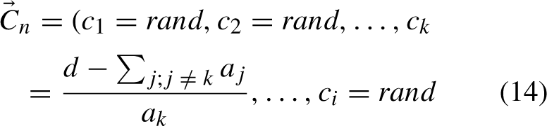
Compute the cruising vector for Golden Eagle ‘n’ in iteration ^′t′ by using random values within the [0, 1] range. This steers the population away from prior recollections and enriches GEO’s exploration.

•Transitioning to Fresh Roles

Golden eagles possess both attack and cruise motion vectors. For golden eagle nduring iterationt, the step vector is determined by Equation (15).

Δ x_{n} = {\vec{r}}_{1} p_{a} \frac{\vec{A_{n}}}{∥ \vec{A_{n}} ∥} + {\vec{r}}_{2} p_{c} \frac{{\vec{C}}_{n}}{∥ {\vec{C}}_{n} ∥}

(15)

During repetition ‘t,’ the navigation of golden eagles is impacted by crucial factors 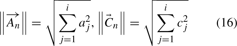$p_{a}^{t}$ and $p_{c}^{t}$ , coupled with random vectors ${\vec{r}}_{1}$ and ${\vec{r}}_{2}$ in the [0, 1] range. The functions of p_aand p_c will undergo additional examination while $∥ {\vec{C}}_{n} ∥$ and $∥ \vec{A_{n}} ∥$ represent norms of Euclidean, as calculated for the attack and cruise vectors through Equation (16):

∥ \vec{A_{n}} ∥ = \sqrt{\sum_{j = 1}^{i} a_{j}^{2}}, ∥ {\vec{C}}_{n} ∥ = \sqrt{\sum_{j = 1}^{i} c_{j}^{2}}

(16)

In iteration (t + 1) , the golden eagles’ locations are determined by merging the step vector computed in iteration t with their positions from iteration t.

x^{t + 1} = x^{t} + Δ x_{i}^{t}

(17)

Golden eagles improve their locations through the coefficients in Equation (15), namely, $p_{a}^{t}$ and $p_{c}^{t}$ , as they simultaneously update their memory by evaluating the quality of their positions during every repetition.

•Shifting from Exploratory to Exploitative Activities

The optimization strategy employed by the Golden Eagles comprises an initial soaring stage, succeeded by a hunting phase, and offers adaptability through the utilization of the parameters p_a and p_c.

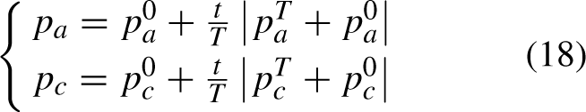
{\begin{matrix} p_{a} = p_{a}^{0} + \frac{t}{T} | p_{a}^{T} + p_{a}^{0} | \\ p_{c} = p_{c}^{0} + \frac{t}{T} | p_{c}^{T} + p_{c}^{0} | \end{matrix}

(18)

Within the mathematical representation, the symbol t denotes the current iterative step, and T represents the upper limit for the number of iterations. The variables $p_{a}^{0}$ and $p_{a}^{T}$ represent the initial and final values for the attack inclination (p_a), while $p_{c}^{0}$ and $p_{c}^{T}$ signify the initial and terminal phases of the cruising propensity (p_c). As per the forthcoming experiments, it is apparent that the suggested parameter settings are $[p_{a}^{0}$ and $p_{a}^{T}$ ] = [0.5, 2] and [ $p_{c}^{0}$ and $p_{c}^{T}$ ]= [1, 0.5]. Throughout iterations, p_a progressively rises from 0.5to2, whereas p_c continuously declines from 1 to 0.5. It is worth mentioning that Equation (18) employs a linear approach for parameter adaptation, although alternative methods like logarithmic or other functions are feasible choices. It is important to note that r₁ and r₂ represent stochastic values within the [0, 1].

2.4 Performance evaluation metrics

Within this investigation, the efficacy of prediction algorithms underwent a meticulous assessment utilizing an extensive set of five critical performance metrics, as reported in Table 2.

Table 2
Performance evaluation metrics

Formula Definition NO.

$R^{2} = {(\frac{\sum_{i = 1}^{n} (T_{i} - \bar{T}) (H_{i} - \bar{H})}{\sqrt{[\sum_{i = 1}^{n} {(T_{i} - \bar{H})}^{2}] [\sum_{i = 1}^{n} {(H_{i} - \bar{H})}^{2}]}})}^{2}$ Coefficient of Determination (19)

$RMSE = \sqrt{\frac{\sum_{i = 1}^{n} {(H_{i} - T_{i})}^{2}}{n}}$ Root Mean Square Error (20)

$MAE = \frac{1}{n} \sum_{i = 1}^{n} ∥ H_{i} - T_{i} ∥$ Mean Absolute Error (21)

$n 10 - index = \frac{n 10}{n}$ n-10 index (22)

$SI = \frac{RMSE}{T_{i}}$ Scatter Index (23)

Formula	Definition	NO.
$R^{2} = {(\frac{\sum_{i = 1}^{n} (T_{i} - \bar{T}) (H_{i} - \bar{H})}{\sqrt{[\sum_{i = 1}^{n} {(T_{i} - \bar{H})}^{2}] [\sum_{i = 1}^{n} {(H_{i} - \bar{H})}^{2}]}})}^{2}$	Coefficient of Determination	(19)
$RMSE = \sqrt{\frac{\sum_{i = 1}^{n} {(H_{i} - T_{i})}^{2}}{n}}$	Root Mean Square Error	(20)
$MAE = \frac{1}{n} \sum_{i = 1}^{n} ∥ H_{i} - T_{i} ∥$	Mean Absolute Error	(21)
$n 10 - index = \frac{n 10}{n}$	n-10 index	(22)
$SI = \frac{RMSE}{T_{i}}$	Scatter Index	(23)

Here, n corresponds to the total number of data points, T_i and H_isymbolize the test and predicted results, respectively, $\bar{T}$ and $\bar{H}$ represent the averages of the test and prediction result values.

3 Results and discussion

3.1 Results of evaluation metrics

Table 3 summarizes performance metrics, encompassing R², RMSE, MAE, n10-index, and SI, across all prediction models applied to the training, validation, and testing datasets. Subsequent analysis delves into a detailed evaluation of the model’s predictive accuracy in estimating the HL:

Table 3
The result of developed models for DT

Model Phase Index values

RMSE R ² MAE n10-index SI

DT Train 1.522 0.978 1.317 0.717 0.068

Validation 1.808 0.968 1.522 0.643 0.084

Test 1.780 0.970 1.501 0.704 0.077

All 1.608 0.975 1.375 0.704 0.072

DTFO Train 0.691 0.996 0.526 0.970 0.031

Validation 1.165 0.987 0.910 0.948 0.054

Test 1.133 0.988 0.869 0.991 0.049

All 0.854 0.994 0.635 0.970 0.038

DTGE Train 1.149 0.987 0.983 0.838 0.051

Validation 1.516 0.978 1.297 0.722 0.071

Test 1.645 0.973 1.390 0.800 0.071

All 1.294 0.984 1.091 0.815 0.058

Model	Phase	Index values
DT	Train	1.522	0.978	1.317	0.717	0.068
	Validation	1.808	0.968	1.522	0.643	0.084
	Test	1.780	0.970	1.501	0.704	0.077
	All	1.608	0.975	1.375	0.704	0.072
DTFO	Train	0.691	0.996	0.526	0.970	0.031
	Validation	1.165	0.987	0.910	0.948	0.054
	Test	1.133	0.988	0.869	0.991	0.049
	All	0.854	0.994	0.635	0.970	0.038
DTGE	Train	1.149	0.987	0.983	0.838	0.051
	Validation	1.516	0.978	1.297	0.722	0.071
	Test	1.645	0.973	1.390	0.800	0.071
	All	1.294	0.984	1.091	0.815	0.058

•

The R² values for all network models vary from 0.968 (noted in the DT single model during validation) to 0.996 (achieved in the training phase of the DTFO ensemble model). These results emphasize the substantial accuracy achieved by the developed models. The DTFO model stands out as the best model due to its R² value being closest to 1, with a difference of 1.8% compared to the DT model and 0.9% compared to the DTGE model during the training phase.

•

In error analysis, the DTFO model outperforms other models with RMSE values approximately two times lower than the DT model and 1.5 times lower than the DTGE model. This highlights the DTFO model’s superior predictive accuracy and significantly reduced discrepancies between predicted and actual values compared to the other models.

•

The n10-index metric assesses the proportion of models with error values below the 10 percent threshold. The results indicate that during the training phase of DTFO, 97% of its models met this criterion, while the testing phase demonstrated 99.1% compliance. In contrast, DTGE had a lower percentage of models below the 10 percent threshold during the training phase, with 83.8%, and a higher proportion during the testing phase, reaching 80% compared to the corresponding testing results for DTGE.

•

SI is a valuable tool for gauging the dispersion or variability of data points within a dataset. Notably, a lower SI value signifies less divergence among the data points, highlighting superior model performance. This trend is evident when examining the DTFO model, which boasts an SI value of 0.031. This value outperforms DTGE by 39.21% and surpasses the DT single model by 54.41%, reaffirming its prowess in minimizing data spread and enhancing predictive accuracy.

3.2 Comparative analysis

In Fig. 3, a reference line, y = x, along with two lines, y = 1.1x, and y = 0.9x, incorporated to expedite the identification of the optimal model. Based on the data distribution close to the center line, it becomes evident that the DTFO model is the most favorable. This assertion is substantiated by the observation that the data points of the DTFO model exhibit significantly reduced dispersion as they approach the vicinity of the designated lines compared to the other models. Upon scrutinizing the remaining two figures and assessing the dispersion of data points between the reference lines, a hierarchical ranking of model performance emerges. After the DTFO model, the DTGE model takes the second position in performance, revealing a comparatively inferior performance compared to the best model. In contrast, the DT single model, when compared to the other models, exhibits the highest degree of data dispersion, indicating its comparatively weaker performance.

Fig. 3

Plotting the dispersion of evolved ensemble models.

In Fig. 4, three plots are presented, of which two pertain to error metrics, while the third is associated with the R² values. The representation takes the form of a column chart, where, concerning error metrics, a shorter column corresponds to superior model performance. In the case of R² values, a taller column signifies enhanced model performance. Based on the elucidations offered, it becomes evident that in the RMSE and MAE charts, the DT model exhibits the tallest columns, signifying its comparatively weak performance when juxtaposed with the other models. Conversely, in the R² chart, the tallest column corresponds to DTFO, which underlines the model’s superiority compared to the other alternatives.

Fig. 4

Stacked column plot to compare the developed models by presented metrics.

Figures 5 and 6 depict the error values of three models (DTFO, DTGE, and DT) by utilizing two distinct visualization formats: the distribution-rug plot and the violin with quartile plot. As illustrated in Fig. 5, it is apparent that the DT model exhibits a frequency of approximately 0.05, the DTFO model has a frequency of around 0.15, and the DTGE model is associated with a frequency of about 0.06 all of the frequencies are effectively converging to a near-zero percentage of error. Consequently, the DTFO model emerges as the most favorable model due to its highest frequency compared to the other models. According to the visual representation as Fig. 6, an analysis of error percentages reveals notable distinctions among the DT, DTGE, and DTFO models. Specifically, the DT and DTGE models exhibit error percentages ranging from approximately 40% to –35%. In contrast, the DTFO model demonstrates a narrower error range, falling within the interval of approximately 20% to –10%.

Fig. 5

The error percentage of the models is based on the distribution-rug plot.

Fig. 6

The violin with quartile plot errors of proposed models.

Based on these two types of plots, to provide a more nuanced understanding of model performance, it is imperative to underscore that a lower error rate indicates superior model performance. So, the DTFO model emerges as the most proficient performer, as its error percentage range is closer to zero. This observation underscores the DTFO model’s ability to generate predictions with higher accuracy than the DT and DTGE models. Consequently, when considering the quality of model outcomes, the DTFO model outshines its counterparts by demonstrating superior predictive accuracy, enhancing its utility in practical applications.

3.3 Wilcoxon test

The Wilcoxon test [45] was utilized to evaluate the relative effectiveness of three models: DT, DTFO, and DTGE. By analyzing the test outcomes, including the p-values and statistics for every model pair, valuable insights into their statistical significance were obtained. Table 4 displays the outcomes of the Wilcoxon test, indicating that there is no statistically significant distinction in performance between DT and DTGE (p-value = 0.7183, Statistic = 143539), as well as between DT and DTFO (p-value = 0.5041, Statistic = 145429.5). These results imply similar performance among the model pairs. Nonetheless, the assessment between DTFO and DTGE indicates a slightly noteworthy difference (p-value = 0.1771, Statistic = 139346). Although the findings do not meet the usual thresholds for significance, they hint at a possible distinction worth exploring further. To summarize, the Wilcoxon test indicates similar performance between DT and DTGE, as well as between DT and DTFO. However, there is a slight but noteworthy difference between DTFO and DTGE, underscoring the importance of careful interpretation and the potential for deeper investigation.

Table 4
Results of the Wilcoxon Test

Difference of models Parameter

p_value Statistic

DT vs DTFO 0.5041 143539

DT vs DTGE 0.7183 145429.5

DTFO vs DTGE 0.1771 139346

Difference of models	Parameter
DT vs DTFO	0.5041	143539
DT vs DTGE	0.7183	145429.5
DTFO vs DTGE	0.1771	139346

3.4 Comparison between previous studies and present one

Table 5 presents the findings of prior research endeavors in Heating Load prediction, providing a comprehensive benchmark for comparison with the current study. Among the three models documented in this table from previous research, the GPR model, as presented in the study by Roy et al. [46], demonstrated the highest performance, boasting an R² of 0.99 and an RMSE of 0.059. As elaborated in Sections 3.1 and 3.2, the investigation underscores the superior performance of the DTFO model during the training phase, yielding impressive metric scores with an R² value of 0.996 and an RMSE of 0.691. This dual excellence in pivotal metrics firmly establishes the DTFO model in the study as surpassing its counterparts, emphasizing its efficacy in predicting Heating Load.

Table 5
Comparing the results of the present study with previous studies

Articles Models Models’ performance

RMSE R ²

Roy et al. [46] GPR 0.059 0.99

Gong et al. [47] GBM 0.1929 0.9882

Afzal et al. [48] MLP 1.4122 0.9806

Present Study DTFO (DT + FO) 0.691 0.996

Articles	Models	Models’ performance
Roy et al. [46]	GPR	0.059	0.99
Gong et al. [47]	GBM	0.1929	0.9882
Afzal et al. [48]	MLP	1.4122	0.9806
Present Study	DTFO (DT + FO)	0.691	0.996

4 Conclusion

In summary, in the field of building energy management, this study examined the critical requirement for precise energy consumption predictions and the evaluation of retrofit techniques. It has traditionally been difficult to predict building energy use accurately because of a variety of variables, including building attributes, energy systems, weather patterns, and tenant behavior. Although physics-based simulations provided insightful information, their accuracy depended on the availability of thorough data and intricate modeling. In response to these difficulties, this research investigated the potential of machine learning approaches, concentrating on Decision Tree models, by using the ever-increasing amount of publicly available building energy data. The results revealed that the DTFO (Decision Tree optimized with Fox Optimization) model emerged as the top-performing model among the other two alternatives. The DTFO model displayed an impressive correlation with the actual measured HL, achieving a high R² value of 0.996, surpassing DT and DTGE (Decision Tree optimized by Golden Eagle optimizer) by 1.8% and 0.9%, respectively. Notably, the DTFO model also showcased superior accuracy compared to the other models, evident through its minimal RMSE value of 0.691. This translated to a substantial 54.59% reduction compared to DT and a 39.86% decrease relative to DTGE in RMSE values. This underscores the considerable promise of machine learning, as demonstrated by DTFO, to greatly improve the accuracy of energy consumption predictions. Therefore, it gives stakeholders more influence over energy-saving and retrofit solutions, supporting the main goals of environmentally friendly building operations and sustainability.

References

Ürge-Vorsatz

Cabeza

L.F.

Serrano

Barreneche

Petrichenko

, Heating and cooling energy trends and drivers in buildings, Renewable and Sustainable Energy Reviews41 (2015), 85–98.

Kusiak

, Cooling output optimization of an air handling unit, Appl Energy87 (2010), 901–909.

Luo

Hong

Jia

Weng

, Data analytics and optimization of an ice-based energy storage system for commercial buildings, Appl Energy204 (2017), 459–475.

Pedersen

Stang

Ulseth

, Load prediction method for heat and electricity demand in buildings for the purpose of planning for mixed energy distribution systems, Energy Build40 (2008), 1124–1134.

Xue

Wang

Sun

Xiao

, An interactive building power demand management strategy for facilitating smart grid optimization, Appl Energy116 (2014), 297–310.

Chaganti

Rustam

Daghriri

de la

Díez

Mazón

J.L.V.

Rodríguez

C.L.

Ashraf

, Building heating and cooling load prediction using ensemble machine learning model, Sensors22 (2022), 7692.

Crawley

D.B.

Lawrie

L.K.

Pedersen

C.O.

Winkelmann

F.C.

, Energy plus: Energy simulation program, ASHRAE J42 (2000), 49–56.

Berardi

Jafarpur

, Assessing the impact of climate change on building heating and cooling energy demand in Canada, Renewable and Sustainable Energy Reviews121 (2020), 109681.

U. IEA, Global energy review 2020, Ukraine.[Online] Https://Www.Iea.Org/Countries/Ukraine [Accessed: 2020-09-10] (2020).

10.

Bourdeau

qiang Zhai

Nefzaoui

Guo

Chatellier

, Modeling and forecasting building energy consumption: A review of data-driven techniques, Sustain Cities Soc48 (2019), 101533.

11.

Evcil

, An estimation of the residential space heating energy requirement in Cyprus using the regional average specific heat loss coefficient, Energy Build55 (2012), 164–173.

12.

Nakhaees Sharif

Keshavarz Saleh

Afzal

Shoja Razavi

Fadaei Nasab

Kadaei

, Evaluating and identifying climatic design features in traditional Iranian architecture for energy saving (case study of residential architecture in northwest of Iran), Complexity2022 (2022).

13.

behnam Sedaghat Tejani

G.G.

Kumar

, Predict the Maximum Dry Density of soil based on Individual and Hybrid Methods of Machine Learning, Advances in Engineering and Intelligence Systems002 (2023). https://doi.org/10.22034/aeis.2023.414188.1129.

14.

Chen

Ngai

E.W.T.

Gou

Zhang

, Prediction of hotel booking cancellations: Integration of machine learning and probability model based on interpretable feature interaction, Decis Support Syst170 (2023), 113959.

15.

Zhang

Gou

Chen

, An online reviews-driven method for the prioritization of improvements in hotel services, Tour Manag87 (2021), 104382.

16.

Breiman

, Statistical modeling: The two cultures (with comments and a rejoinder by the author), Statistical Science16 (2001), 199–231.

17.

Wei

Zhang

Shi

Xia

Pan

Han

Zhao

, A review of data-driven approaches for prediction and classification of building energy consumption, Renewable and Sustainable Energy Reviews82 (2018), 1027–1047.

18.

Abd Alla

Bianco

Tagliafico

L.A.

Scarpa

, Life-cycle approach to the estimation of energy efficiency measures in the buildings sector, Appl Energy264 (2020), 114745.

19.

Zhao

Liu

, A hybrid method of dynamic cooling and heating load forecasting for office buildings based on artificial intelligence and regression analysis, Energy Build174 (2018), 293–308.

20.

Di Foggia

, Energy efficiency measures in buildings for achieving sustainable development goals, Heliyon4 (2018).

21.

Shi

Jabari

Anvari-Moghaddam

Mohammadpourfard

Mohammadi-ivatloo

, Risk-constrained optimal chiller loading strategy using information gap decision theory, Applied Sciences9 (2019), 1925.

22.

Kotsiantis

S.B.

, Decision trees: A recent overview, Artif Intell Rev39 (2013), 261–283.

23.

Akbarzadeh

M.R.

Ghafourian

Anvari

Pourhanasa

Nehdi

M.L.

, Estimating Compressive Strength of Concrete Using Neural Electromagnetic Field Optimization, Materials16 (2023), 4200.

24.

Chen

Xia

Jiang

Liu

Sun

, Short-term load forecasting based on deep learning for end-user transformer subject to volatile electric heating loads, IEEE Access7 (2019), 162697–162707.

25.

Roy

S.S.

Samui

Nagtode

Jain

Shivaramakrishnan

Mohammadi-Ivatloo

, Forecasting heating and cooling loads of buildings: A comparative performance analysis, J Ambient Intell Humaniz Comput11 (2020), 1253–1264.

26.

Abdelkader

Al-Sakkaf

Ahmed

, A comprehensive comparative analysis of machine learning models for predicting heating and cooling loads, Decision Science Letters9 (2020), 409–420.

27.

Mokeev

V.V

, Prediction of heating load and cooling load of buildings using neural network, in: 2019 International Ural Conference on Electrical Power Engineering (UralCon), IEEE, (2019), pp. 417–421.

28.

Moradzadeh

Mansour-Saatloo

Mohammadi-Ivatloo

Anvari-Moghaddam

, Performance evaluation of two machine learning techniques in heating and cooling loads forecasting of residential buildings, Applied Sciences10 (2020), 3829.

29.

Song

Zhang

Xue

Gao

Jiang

, Predicting hourly heating load in a district heating system based on a hybrid CNN-LSTM model, Energy Build243 (2021), 110998.

30.

Yao

, A machine-learning-based approach to predict residential annual space heating and cooling loads considering occupant behaviour, Energy212 (2020), 118676. https://doi.org/10.1016/j.energy.2020.118676

31.

khiavi

B.S.A.J.

, B.N.E.K.A.R.T.K. hadi Sadaghat, The Utilization of a Naive Bayes Model for Predicting the Energy Consumption of Buildings, Journal of Artificial Intelligence and System Modelling01 (2023). https://doi.org/10.22034/JAISM.2023.422292.1003.

32.

Wong

S.L.

Wan

K.K.W.

Lam

T.N.T.

, Artificial neural networks for energy analysis of office buildings with daylighting, Appl Energy87 (2010), 551–557.

33.

Paudel

Elmtiri

Kling

W.L.

Le Corre

Lacarrière

, Pseudo dynamic transitional modeling of building heating energy demand using artificial neural network, Energy Build70 (2014), 81–93.

34.

Chou

J.-S.

Bui

D.-K.

, Modeling heating and cooling loads by artificial intelligence for energy-efficient building design, Energy Build82 (2014), 437–446.

35.

Schiavon

Lee

K.H.

Bauman

Webster

, Influence of raised floor on zone design cooling load in commercial buildings, Energy Build42 (2010), 1182–1191.

36.

Fan

Wang

Gang

, Assessment of deep recurrent neural network-based strategies for short-term building energy predictions, Appl Energy236 (2019), 700–710.

37.

Zhong

Wang

Jia

, Vector field-based support vector regression for building energy consumption prediction, Appl Energy242 (2019), 403–414.

38.

Zhou

Moayedi

Bahiraei

Lyu

, Employing artificial bee colony and particle swarm techniques for optimizing a neural network in prediction of heating and cooling loads of residential buildings, J Clean Prod254 (2020), 120082.

39.

Pessenlehner

Mahdavi

, Building morphology, transparence, and energy performance, na, 2003.

40.

Karbassi

Mohebi

Rezaee

Lestuzzi

, Damage prediction for regular reinforced concrete buildings using the decision tree algorithm, Comput Struct130 (2014), 46–56.

41.

Erdal

H.I.

, Two-level and hybrid ensembles of decision trees for high performance concrete compressive strength prediction, Eng Appl Artif Intell26 (2013), 1689–1697.

42.

Ahmad

Farooq

Niewiadomski

Ostrowski

Akbar

Aslam

Alyousef

, Prediction of compressive strength of fly ash based concrete using individual and ensemble algorithm, Materials14 (2021), 794.

43.

Połap

Woźniak

, Red fox optimization algorithm, Expert Syst Appl166 (2021).https://doi.org/10.1016/j.eswa.2020.114107

44.

Mohammadi-Balani

Nayeri

M.D.

Azar

Taghizadeh-Yazdi

, Golden eagle optimizer: A nature-inspired metaheuristic algorithm, Comput Ind Eng152 (2021), 107050.

45.

Jiang

M.-R.

M.-W.

Hong

W.-C.

R.-Z.

, A floating offshore platform motion forecasting approach based on EEMD hybrid ConvLSTM and chaotic quantum ALO, Appl Soft Comput (2023), 110487.

46.

Roy

S.S.

Samui

Nagtode

Jain

Shivaramakrishnan

Mohammadi-Ivatloo

, Forecasting heating and cooling loads of buildings: A comparative performance analysis, J Ambient Intell Humaniz Comput11 (2020), 1253–1264.

47.

Gong

Bai

Qin

Wang

Yang

Wang

, Gradient boosting machine for predicting return temperature of district heating system: A case study for residential buildings in Tianjin, Journal of Building Engineering27 (2020), 100950.

48.

Afzal

Ziapour

B.M.

Shokri

Shakibi

Sobhani

, Building energy consumption prediction using multilayer perceptron neural network-assisted models; comparison of different optimization algorithms, Energy (2023), 128446. https://doi.org/10.1016/j.energy.2023.128446.

Variables	Indicators
	Category	Min	Max	Avg	St . Dev .
RelativeCompactness	Input	0.62	0.98	0.764	0.106
SurfaceArea	Input	514.5	808.5	671.7	88.09
WallArea	Input	245	416.5	318.5	43.63
RoofArea	Input	110.3	220.5	176.6	45.17
Overall, Height	Input	3.5	7	5.25	1.751
Orientation	Input	2	5	3.5	1.119
GlazingArea	Input	0	0.4	0.234	0.133
GlazingAreaDistribution	Input	0	5	2.813	1.551
Heating	Output	6.01	43.1	22.31	10.09

Model	Phase	Index values
		RMSE	R ²	MAE	n10-index	SI
DT	Train	1.522	0.978	1.317	0.717	0.068
	Validation	1.808	0.968	1.522	0.643	0.084
	Test	1.780	0.970	1.501	0.704	0.077
	All	1.608	0.975	1.375	0.704	0.072
DTFO	Train	0.691	0.996	0.526	0.970	0.031
	Validation	1.165	0.987	0.910	0.948	0.054
	Test	1.133	0.988	0.869	0.991	0.049
	All	0.854	0.994	0.635	0.970	0.038
DTGE	Train	1.149	0.987	0.983	0.838	0.051
	Validation	1.516	0.978	1.297	0.722	0.071
	Test	1.645	0.973	1.390	0.800	0.071
	All	1.294	0.984	1.091	0.815	0.058

Difference of models	Parameter
	p_value	Statistic
DT vs DTFO	0.5041	143539
DT vs DTGE	0.7183	145429.5
DTFO vs DTGE	0.1771	139346

Heating load prediction in buildings using decision tree machine learning method

Abstract

Keywords

1 Introduction

2 Materials and methods

2.1 Data collection

2.2.1 Decision Tree (DT)

2.3.1 Red Fox Optimization (FO)

3.1 Results of evaluation metrics

Table 4 Results of the Wilcoxon Test Difference of models Parameter p_value Statistic DT vs DTFO 0.5041 143539 DT vs DTGE 0.7183 145429.5 DTFO vs DTGE 0.1771 139346

Table 5 Comparing the results of the present study with previous studies Articles Models Models’ performance RMSE R 2 Roy et al. [46] GPR 0.059 0.99 Gong et al. [47] GBM 0.1929 0.9882 Afzal et al. [48] MLP 1.4122 0.9806 Present Study DTFO (DT + FO) 0.691 0.996

References

Table 4
Results of the Wilcoxon Test

Difference of models Parameter

p_value Statistic

DT vs DTFO 0.5041 143539

DT vs DTGE 0.7183 145429.5

DTFO vs DTGE 0.1771 139346

Table 5
Comparing the results of the present study with previous studies

Articles Models Models’ performance

RMSE R ²

Roy et al. [46] GPR 0.059 0.99

Gong et al. [47] GBM 0.1929 0.9882

Afzal et al. [48] MLP 1.4122 0.9806

Present Study DTFO (DT + FO) 0.691 0.996