Computational optimization of a 3D printed collimator

Abstract

This contribution describes the computational methodology behind an optimization procedure for a scattered beam collimator. The workflow includes producing a file that can be manufactured via additive methods. A conical collimator, optimized for neutron diffraction experiments in a high pressure clamp cell, is presented as an example. In such a case the scattering from the sample is much smaller than that of the pressure cell. Monte Carlo Ray tracing in MCViNE was used to model scattering from a Si powder sample and the cell. A collimator was inserted into the simulation and the number and size of channels were optimized to maximize the rejection of the parasitic signal coming from the complex sample environment. Constraints, provided by the additive manufacturing process as well as a specific neutron diffractometer, were also included in the optimization. The source code and the tutorials are available in c3dp (Islam (2019)).

Keywords

High pressure optimization Monte Carlo simulation 3D printing

1. Introduction

Scattered beam collimation is an effective way to remove scattering from materials in the beam (e.g. sample environment equipment) that are not at the sample position [6]. Typically a collimator is designed for an instrument with the collimation chosen to work well for most standard equipment [10,18,29,34]. Once a collimator’s scientific specifications are chosen the device goes to engineering design and manufacture. However, background rejection, more tailored to a specific experiment, can be achieved by optimizing a collimator to a specific sample environment. For this to be practical, the effort from experiment design through to a usable device must be reduced. This contribution summarizes a way to reduce this effort.

Here we show a new avenue for custom-made collimators to overcome this challenge. Specifically, an automated work-flow has been developed to design a custom collimator, optimized for a given sample environment and manufacturing constraints. The end result is a file ready for 3D printing. To perform the optimization, the sample environment is included in a detailed model for a Monte Carlo ray tracing simulation of the instrument. A collimator is inserted into the beamline model and its parameters optimized to produce the best configuration for this application. Once the collimator has been optimized in the computer, the computer model is transformed directly into an .stl file for production via additive manufacturing.

To demonstrate this technique, the optimization of a collimator for a clamp cell [32] on the SNAP high pressure diffractometer [5] of the Spallation Neutron Source [27] is chosen. SNAP’s key advantages lie in the fact that the high flux beam is focused into a very small area, the detector positions can be adjusted, and its sample position is extremely accessible thus accommodating to complex sample environments. High pressure environments are ideal to demonstrate such collimation as they contain pressure cell material in the beam upstream of the sample and in the scattered beam between the sample and detectors. Particularly, the pressure cell, consists of more material than sample and completely surrounds the sample. Therefore, no unobstructed view of the sample is inherently possible. Hence every measurement is contaminated by scattered neutrons from the sample environment. Our approach to custom collimation modelling places the device much closer to the sample than one designed around the instrument alone, allowing for more effective collimation. Section 2 describes the details of the simulation.

The optimization parameters include number of channels, channel-size and materials of the collimator. An optimized collimator will maximize the sample signal to background ratio without sacrificing too much neutron flux. Thus, the optimization must strike a balance between improving relative sample signals and minimizing the loss of intensities, while staying within the constraints placed upon it by the 3D printing techniques and the neutron instrument. In Section 3, the design and optimization of the conic divergent collimator will be discussed, including the mounting facility of the collimator. Such an optimization workflow is composed of many parts that are summarized in Fig. 1.

Fig. 1.

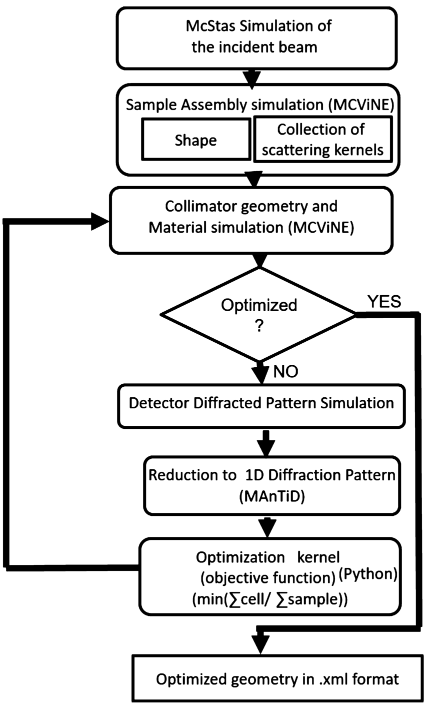
Collimator optimization workflow.

Furthermore an intuitive understanding of the collimator operation can be obtained through examining the gauge volume of the sample observed by the detector via the collimator. Such a calculation and our specific implementation will be described in Section 4.

As with any manufacturing process, additive manufacturing provides unique constraints that must be considered in the design of a device. Section 5 describes the constraints and printing processes.

Finally initial comparisons between measurements and simulations with the collimator are shown in Section 6. These demonstrate the effectiveness of the collimator in reducing background scattering from complex sample environment.

2. Simulation of beamline and pressure cell

As mentioned above, the optimization workflow uses simulations of a clamp cell on SNAP [5], a medium-resolution diffractometer optimized for small samples such as those in high pressure environments. A schematic of the SNAP instrument can be found in Fig. 2. The choppers were phased to provide a center wavelength of 2.1 Å with a bandwidth of 0.5–3.54 Å. The beamline is typically operated with its focusing guide in place to focus the beam into a $3 \times 3 {mm}^{2}$ spot. Further incident beam collimation is provided through a 1 mm diameter hexagonal boron nitride collimator directly in front of the pressure cell. SNAP has two movable detectors. For collimator optimization, only the “west” detector was used. For the simulation here, its scattering angle was centered on $55^{\circ}$ .

Monte Carlo neutron ray tracing simulations using MCViNE [22,24] and McStas [36] are performed to estimate the possible improvement in sample signal with an optimized collimator. All parameters (placement of components, chopper disc opening angles, etc.) were taken from engineering drawings of the installed components.

Fig. 2.

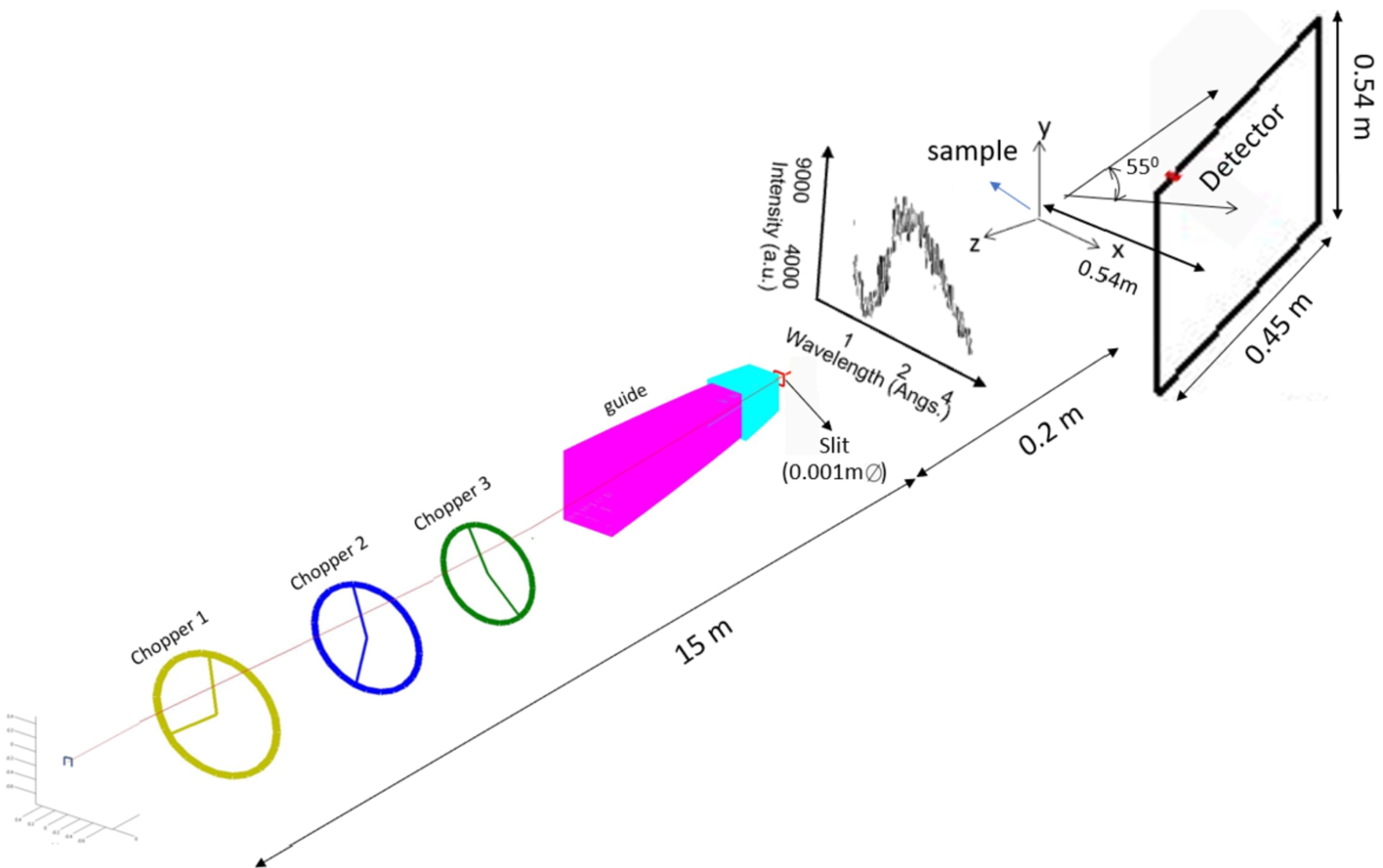
Simulated SNAP layout with sample and detector positions used in the calculation.

The statistics presented here correspond to $10^{9}$ neutron packets generated at the neutron source. The simulated neutron beam, recorded at the sample position, is reused [22] so that neutron packets on the order of $10^{8}$ are incident on the sample, yielding an accuracy of $< 2$ %.

The incident beam on SNAP is modelled using McStas. As a source we used the component SNS_source, which uses input files provided by the SNS neutronics team to simulate the shape of one full spallation pulse [14,25,26]; thereby giving information about the inherent time structure of the neutron beam. A set of three frame overlap choppers (component DiskChopper) provides the wavelength bandwidth one can expect at the real instrument. While a $T_{0}$ -chopper is in the model it was not utilized in the simulations, since the SNS_source gives no information about the prompt pulse a $T_{0}$ -chopper is designed to minimize.

A focusing guide, with the general formula $x = - 9.961091 y^{2}$ and $x = - 12.56984 y^{2}$ for width and height, respectively, transports the beam from source to sample. It starts at 2.8486 m upstream of the sample position (width = 34.7 mm, height = 30.89 mm) and ends 0.5 m upstream of the sample position (width = 16.16 mm, height = 14.38 mm). The neutrons exiting the guide were saved at a point 14.7 m from the source using the McStas Virtual_output command.

MCViNE is then used to model the neutron propagation from the sample to the detectors. The McStas .dat file format, saved in the previous step, is fed into the mcstas2mcvine utility function, included in MCViNE, to convert the neutrons exiting the guide for the subsequent MCViNE simulation.

One advantage of using MCViNE is that it can simulate sample assemblies of multiple materials and complex shapes [22,24,30]. MCViNE supports Constructive Solid Geometry (CSG) [19] to compose complex solid shapes such as the sample assembly. Specifically it uses logical operations on a limited set of simple solid shapes to create complex ones.

Here we used the constructive solid geometry available in MCViNE [17] to model such a complex shape of the collimator and the sample environment. Over the past decade MCViNE development has moved in a direction focusing on complex sample kernels, mostly for inelastic but also some elastic processes, and building the model of the detector from its definition in the Mantid [1] reduction software. In this way, it is optimized for use in analysis of neutron scattering results on existing instruments as is demonstrated in several publications, [9,22–24,28,30,33,37]. In a complimentary manner McStas [36] is a well documented code that runs extremely quickly and allows for quick changes of detector configurations [36]. These features are critical for fast optimization during neutron instrument design, a purpose for which this code has excelled for the past decade [36]. Recently, the Union components [2] have been introduced into McStas and users have started to do complex sample interactions using this feature. Furthermore there are some complex kernels like the IncoherentPhonon_process.comp that in this case could be used to model inelastic background [20]. Additional backgrounds arising from the complex material arrangements such as the texture of the materials can be tackled with either texture.comp module in McStas [20,21] or the LaboSoft s.c. software [31]. Such texture modelling would be useful for the example of a pre-stressed pressure cell as used here. Thus, both packages provide a route to a background component, arising from the material’s texture, currently unaccounted for in our optimization workflow. Since both McStas and MCViNE can read and write intermediate results, the powerful approach we used is not an either/or but leverages a mix of the two codes. We expect to extend this mixed way of working for better simulations in the future.

Here we describe step by step how the geometry of our clamp cell was modeled. Our cell design uses a CuBe insert pressed into an Al sleeve for increased stability [32]. Consequently both of these components are modeled in the simulations. In a measurement, the sample is loaded into a very thin Teflon tube, here only the sample (Si powder) was modeled. Absorption, transmission and scattering probabilities were considered whenever a neutron path intersected a component in the sample environment. The components of the clamp cell are differentiated in the simulation based on their material composition. All of them are cylindrical in shape and share the same axis as shown in Fig. 3(A). Two hollow cylinders are created for the sleeve and the insert and one solid cylinder is created for the sample. The subtraction operation is performed to create hollow cylinders. The geometry of the collimator is also modeled using CSG. The collimator is conical in shape with tightly spaced neutron absorbing blades which are stacked radially in both the vertical and horizontal directions to provide transmitting channels as shown in Fig. 3(B) and (C). The blade surfaces were simulated by rectangular block segments of constant thickness. Here the blades are repeated in both the vertical and horizontal directions which produces a crossed-blade pattern; in other words a grid. Each blade is pitched to focus to where the beam intersects with the center of the sample. These blades define channels of constant angular size along which neutrons may pass. More details of the geometry configuration of collimator is discussed in Section 4.

Fig. 3.

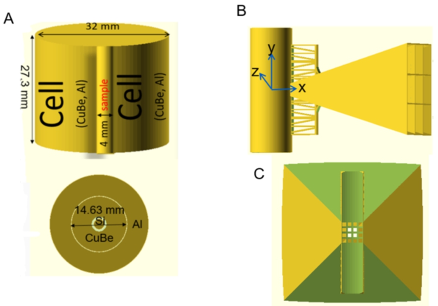
A). Simulated clamp cells. B) and C). Simulated collimator for clamp cell.

The Python geometry script exports an XML file. The XML file is used for multiple purposes as summarized in Fig. 4. First, it is used by the MCViNE simulation to control the ray tracing through the collimator and sample. Second the SCADGen module of MCViNE uses it to convert to a .scad file. Third it is used in the gauge volume calculation. Openscad [35] then can use this .scad file for visualizing the components or conversion to additive manufacturing data formats; specifically .stl, a standard format used for 3D printing.

Fig. 4.

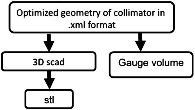
Flowchart showing the uses of .xml file which contains the geometry of optimized collimator.

Table 1

Unit cell structure

Scatterer	atomic percentage	scattering cross section
Al	100	1.503
CuBe	Cu(86), Be(14)	Cu(8.03), Be(7.63)
Si	100	2.167

After the modeling of clamp cell geometry, the unit cell of the scatterer and diffraction scattering kernels are modeled. Table 1 [32] lists the scatterer information. All of them together are included in another XML file called the sample assembly file. The neutrons emitted from the guide, that are saved in the MCViNE .dat file, are fed into the sample assembly and the scattered neutrons are saved. By saving the scattered neutrons, the collimator can be optimized without having to rerun the full simulation. This makes the code more efficient. The scattered neutrons from the sample assembly are fed into the collimator and the neutrons that pass through the collimator are sent to the virtual detector system for reduction and analysis. The interception of simulated scattered neutrons by the SNAP detector system, as defined by the Mantid instrument definition file, were simulated and NeXus files were generated. The NeXus [17] files were reduced using Mantid [1] to obtain the diffraction pattern (I(d)). Similar to the clamp cell, there is another .XML file that defines the material in the collimator. These can be easily swapped so a collimator with either absorbing $B_{4} C$ or incoherently scattering hydrogen, as present in hydrocarbons, can be chosen as the material of the collimator.

3. Collimator design and optimization

As mentioned in the introduction, Fig. 1 summarizes the workflow used to optimize a collimator. In this example here, first the incident beam to sample for SNAP is modeled using McStas [36]. Next, the neutron interaction with the sample assembly, composed of the pressure cell and the sample, is modeled with MCViNE [22]. In the third step, the collimator for the scattered neutrons from sample assembly is modeled using MCViNE. Next, a comparison to the optimization metric, to be described shortly, is performed. If the optimum performance is not achieved, the neutrons coming from the collimator are saved. In the fifth step, data is reduced. The details of the simulation and reduction steps are described in Section 2. In the sixth step a differential evolution (DE) algorithm from the SciPy [15] library was used to optimize the collimator geometry with the objective of minimizing the integrated cell peaks to integrated sample peaks ratio. Once the optimized collimator geometry is determined, it is saved to an .xml file as the last step of the workflow. Further details about optimization are described below. The code used to perform the optimization is called c3dp [12].

The design of the conical collimator system used for this experiment is based on straightforward geometrical considerations, which we briefly discuss with the help of Fig. 5. A conical collimator can be described by 9 parameters: the length of the blades, (L); the horizontal acceptance angle, ( $θ_{w}$ ); vertical acceptance angle ( $θ_{H}$ ); the number of horizontal channels, ( ${CN}_{h}$ ); the number of vertical channels, ( ${CN}_{v}$ ); the horizontal blade thickness, ( $b_{h}$ ); vertical blade thickness, ( $b_{H}$ ); minimum horizontal channel thickness, ( $t_{w}$ ) and the minimum vertical channel thickness, ( $t_{H}$ ) as shown in Fig. 5, illustrated schematically for a collimator with only 30 channels with one side wall off. With the help of Fig. 5 it is straightforward to derive the following relations: $\begin{array}{l} (1) & θ_{H} (SD, H_{D}) = 2 arctan \frac{H_{D}}{2 SD} \\ (2) & θ_{w} (SD, W_{D}) = 2 arctan \frac{W_{D}}{2 SD} \\ (3) & h ({CN}_{h}, t_{H}, b_{H}) = {CN}_{h} * t_{H} + ({CN}_{h} + 1) * b_{H} \\ (4) & w ({CN}_{w}, t_{w}, b_{w}) = {CN}_{w} * t_{w} + ({CN}_{w} + 1) * b_{w} \\ (5) & F (h, θ_{H}) = \frac{\frac{h}{2}}{tan \frac{θ_{H}}{2}} \\ (6) & H (F, L, θ_{H}) = 2 (L + F) tan \frac{θ_{H}}{2} \\ (7) & W (F, L, θ_{w}) = 2 (L + F) tan \frac{θ_{w}}{2} \\ (8) & θ_{t H} (F, t_{H}) = 2 arctan \frac{t_{H}}{2 F} \\ (9) & θ_{t w} (F, t_{w}) = 2 arctan \frac{t_{w}}{2 F} \\ (10) & b_{n h} = {CN}_{h} + 1 \\ (11) & b_{n w} = {CN}_{w} + 1 \\ (12) & {CN}_{h} = {CN}_{w} \\ (13) & F < F_{max} = \{\begin{matrix} \frac{H_{max}}{2 tan (\frac{θ_{H}}{2})} - L, & if H_{max} > W_{max} \\ \frac{W_{max}}{2 tan (\frac{θ_{w}}{2})} - L, & otherwise \end{matrix} \end{array}$

The collimator function analytically describes the acceptance angle as a function of detector area. However, the acceptance angle is limited to $25^{\circ}$ in both the horizontal and vertical directions by the build volume of the printer.

In order to avoid cracking during the printing process, described below, a workable ratio of the channel gap to blade thickness has to be maintained. Specifically the minimum channel gap is ∼3 mm and the blade thickness is defined to be ∼1 mm. The channel shape is rectangular. These are constraints in the optimization loop.

The ratio of the channel length to its width or height is one of the key parameters determining the efficiency of the collimation. The larger the ratio is the better collimation can be achieved with a given structure (providing the neutron absorption cross section is sufficient). Thus the shorter the collimator, the narrower the transmitting channels must be to obtain the required performance. In order to produce optimal collimation and transmission the number of the channels and their lengths will be varied to be considered as the optimized parameters within the printing constraint of channel size being 3 mm × 3 mm and blade size being 1 mm × 1 mm.

The goal of the optimization of the collimation system is to reduce the pressure cell diffraction peaks intensities, while minimizing the impact on the sample peaks. The function of the optimized collimator is to provide a large surface area over which to detect scattered neutrons from the sample, while restricting the gauge volume to minimize the cell to sample ratio.

In this work we did a preliminary look at the Dakota optimizer [3] and its multiple methods but the ease and simplicity of the DE algorithm in scipy was chosen as it was sufficient for our needs. The workflow presented here could be further optimized by evaluating the performance of other optimization algorithms such as genetic algorithms [11], Particle swarm optimization (PSO) [8] and multi-parents crossover (MPC) [4] algorithms to yield further complementary and more robust results. However, these studies are beyond the scope of the work presented here.

A differential evolution optimization engine was used. The population size and maximum number of iterations were selected to be 5 and 20, respectively. The computer’s clock is tapped to obtain 10 different seeds to initialize the random state of 10 independent optimization runs to achieve the final version of the optimized collimator. The average optimal length of the channel is 152 mm with 0.5 mm standard deviation and the optimal number of channels is 25 in all runs. Therefore, the solution from our optimization procedure is highly reproducible. The optimum length and number of the channels obtained are shown in Fig. 6.

Fig. 5.

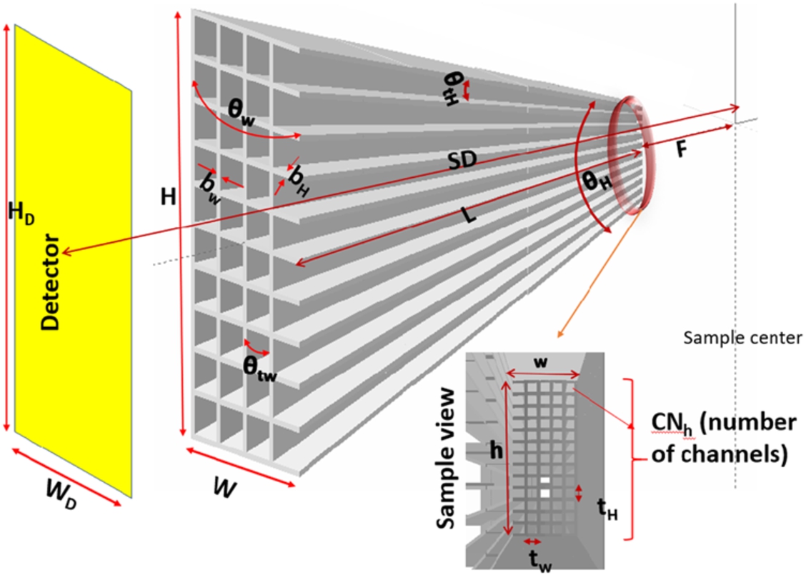
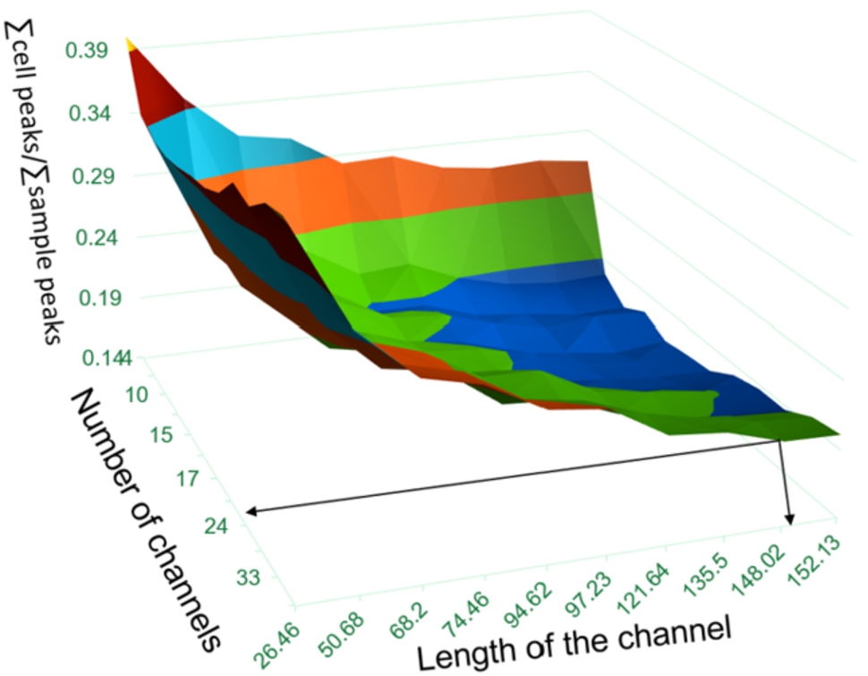
Cross section of conical collimator geometry and parameters: height of the collimator downstream (H), width of the collimator downstream (W), height of the collimator upstream (h), width of the collimator upstream (w), length of the blade (L), horizontal acceptance angle ( $θ_{w}$ ), vertical acceptance angle ( $θ_{H}$ ), collimator upstream distance from sample center (F), horizontal blade thickness ( $b_{w}$ ), vertical blade thickness ( $b_{H}$ ), minimum horizontal channel thickness ( $t_{w}$ ), minimum vertical channel thickness ( $t_{H}$ ).

Fig. 6.

Optimizing curve looking for min $\sum cell peaks / \sum sample peaks$ .

The collimator has a truss support on the top and bottom to mount the collimator to the cell. The purpose of using a truss rather than a solid geometry is to provide stability while printing. Specifically once material is extruded, it immediately starts to cool. If the internal portion of the part cools at a different rate, the part will crack from differential thermal contraction. Therefore the structures must not be too thick. This constraint has been added to the optimization loop.

4. Gauge volume calculation

Gauge volume [7] is defined by the extent of the sample that can be seen on the detector through the collimator. Points at collimator center can be seen 100%. If we move from this point either vertically, horizontally perpendicular to the beam or along the beam, the gauge volume will decrease because the view through some of the collimator channels is obstructed. It has a Gaussian intensity profile in 3D.

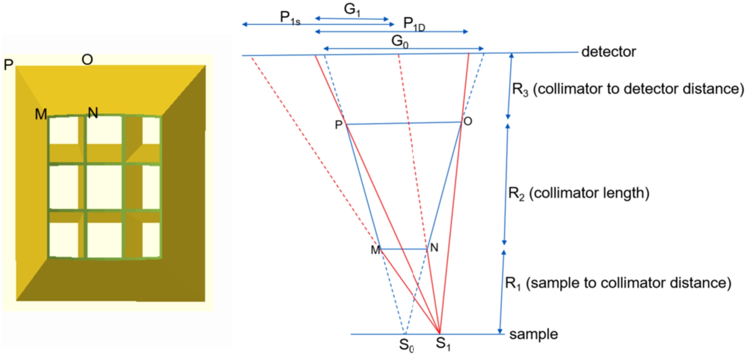
A Python library was written to calculate the Gauge volume. To illustrate how the code works, consider the horizontal plane. If we move perpendicular to the beam, point $S_{1}$ in Fig. 7 can be seen on the detector only in the common segment ( $G_{1}$ ) between the projections of $MN$ ( $P_{1 s}$ ) and $OP$ ( $P_{1 D}$ ), where $MN$ , $OP$ are the upstream and downstream width of the collimator channels. The views are normalized by the maximum view for the sample point at the center of the collimator channel.

Fig. 7.

The left figure shows the 3D view of the collimator and the right figure shows the properties to calculate the gauge volume.

From the model of a single channel the views from all the channels on the detector through collimation can be calculated by summing the contributions from n (number of the channels) rotated sample points (observation points) in front of the single channel which requires a rotation of the observation points about the origin for each channel.

How much of the sample and sample assembly points (cell) that can be viewed on the detector through the collimation is determined by the length of the collimator ( $R_{2}$ ), the proximity of the collimator to the sample ( $R_{1}$ ) and the upstream or downstream width of the collimator channels ( $MN$ or $OP$ ) $\begin{array}{l} (14) & P_{1 s} = 2 S_{1} (1 - \frac{R_{1} + R_{2} + R_{3}}{R_{1}}) \\ (15) & P_{1 D} = 2 S_{1} (1 - \frac{R_{1} + R_{2} + R_{3}}{R_{1} + R_{2}}) \\ (16) & G_{1} = P_{1 D} \cap P_{1 s} \end{array}$

In order to minimize the view of the sample assembly and maximize the view of the sample, the collimator and sample centers must be coincident.

This Python library includes ray tracing code to visualize the Gauge volume. This was achieved through calculation of the detector visibility at each point in the sample region using the vector analysis method described above. Figure 8A shows the calculated gauge volume profile chosen for the optimized collimator. Figures 8B and C show the effect of translations in the vertical to and along the beam directions, respectively. The vertical collimation was designed to be broader than the horizontal collimation to allow for the cylindrical shape of the sample which, as shown in Fig. 3, has a larger height than the diameter. This difference explains the elongated diamond shape. In Fig. 8 A, when the collimator center is aligned to the sample center, integrating the increment in detector view over the sample region shows that it rises to 95% of the collimated value horizontally and 86% vertically.

Figures 8(B) and (C) demonstrate the stringent positioning requirements for the collimator. For example in Fig. 8(C), the sample view was reduced to 6% when placing the collimator 40 mm away from the sample along the beam axis. Placing the collimator as close as possible to the sample keeps the view of the sample’s surroundings on the detector to a minimum, thus retaining the gauge volume shape. In other words, the gauge volume shape is blurred when the collimator is placed further away from the sample. The effect of moving the collimator along the vertical axis is also examined in 8(B). As the sample is cylindrical in shape and has significant height, vertical movement of the collimator on gauge volume has less impact. The absolute value of the sample view did not change but the position is offset along the vertical axis. As long as the vertical movement of the collimator is kept within the sample volume and incident beam volume, it should have a minimal impact on the sample signal to cell signal ratio.

Fig. 8.

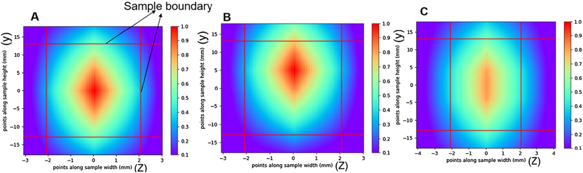
The gauge volume profile in YZ plane of sample region (clampcell + Si) for different configuration of the collimator. The solid line defines the sample region. The intensity scale is relative to maximum gauge volume at the central position of the collimator A) collimator center coincide with sample center. B) Collimator shifted to upward vertical direction C) Collimator is moved away along X axis. Axis configurations are shown in Fig. 3(B).

5. 3D printing

As mentioned in Section 2, the output of the optimization is a .stl file that is used for producing the collimator via additive manufacturing methods. Each additive manufacturing process has its own specific constraints and parameters that need to be varied. We used the constraints for binder jet printing with $B_{4} C$ , but when it came to printing the part to be tested on the neutron beam, we printed the collimator from 1.75 mm polylactic acid (PLA) filament using a Fused Deposition Modeling (FDM) process. We will discuss the constraints that the binder jet process placed on the model and then will summarize the parameters used for the part printed for testing. The main constraints come in the baking step of the binder jet process. Here if there is a thin part intersecting a thick part, the thin part will cool faster than the thick part. This differential thermal contraction can cause the part to crack. Conversely we can not make features too thin because they may break in transporting the model for baking. By performing test prints with the binder jet equipment, we decided to limit the blades thickness to $\sim 1 mm$ with channels no smaller than 3 mm to ensure the manufacturability of the collimator. These constraints were used in the optimization process described in Section 3.

As mentioned above, the .stl file generated by the optimization software was imported into a printer specific version of slic3r [16]. Slic3r is an open source application for converting .stl files into instructions (called g-code) understandable by a 3D printer. Slic3r Prusa Edition version 1.31.6 was used to generate g-code.

6. Experimental results and discussion of the collimator performance

The performance of these collimators was then evaluated on SNAP. The instrument was configured identically to the simulation mentioned in Section 2. As in the model outlined above, the beamline was operated with its guide in place to increase flux on sample. The “west” detector was placed at 50° and standard chopper settings were used (60 Hz, 2.1 Å center wavelength).

A Si sample, which is a NIST powder diffraction standard, was loaded into a 4 mm diameter Teflon tube which in turn, was placed inside the cell.

The clamp cell was placed into the beamline on a sample post and aligned using standard SNAP procedures. The collimator was clamped directly to the cell to ensure its correct alignment with respect to the sample. The collimator was moved to 55° to directly correspond to the simulations detailed above. Additionally an incident beam collimator, made from hBN, was placed directly in front of the cell to give a beam size of 1 mm diameter.

Resulting diffraction data were reduced using standard SNAP procedures. Normalization was thereby performed using a calculated vanadium created via a Mantid algorithm built into the SNAP data analysis procedures. It should be noted that the collimator used here did not cover the entire “west” detector. Thus, the irrelevant portions of the detector were masked during the data reduction.

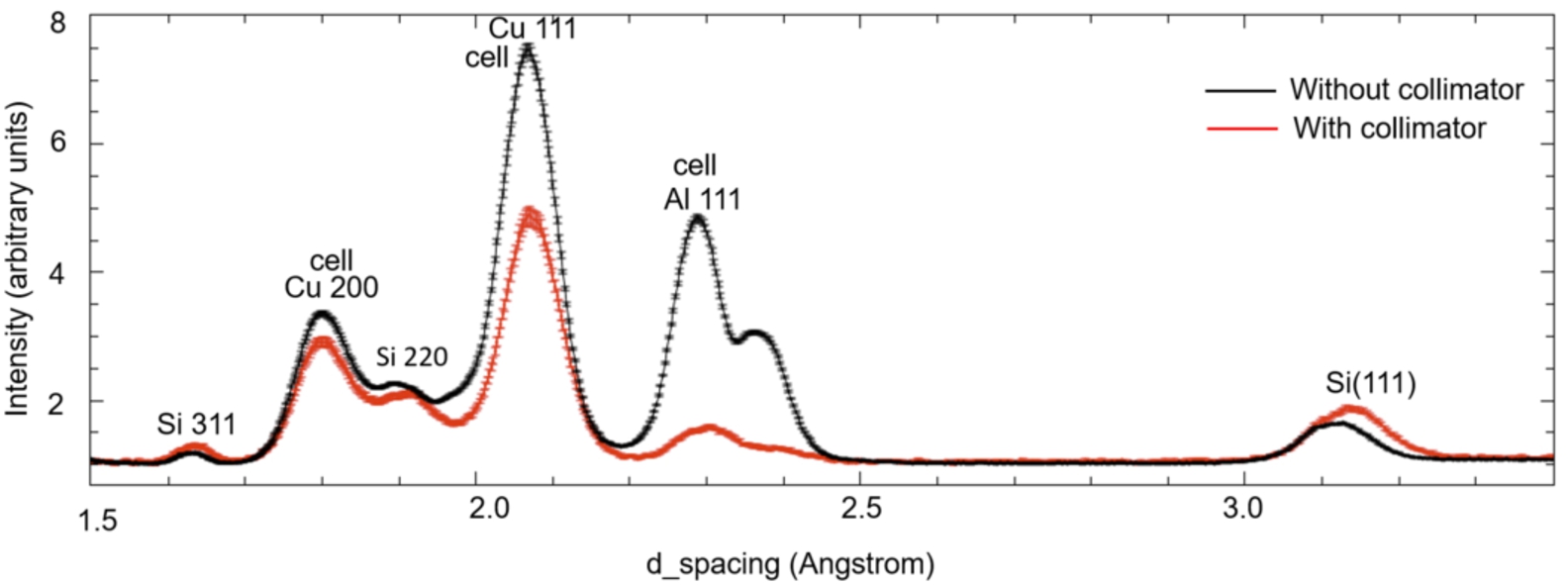
Figure 9 shows the diffraction pattern obtained from the clamp cell and the Si powder both with (red line) and without (black line) the collimator.

The effect of the collimator is very clear. For example, the Al 111 peak from the cell, centered at 2.3 Å, is significantly suppressed and the Si 311 peak, centered at 1.6 Å, is more easily observed when the collimator is in place.

Fig. 9.

Experimental diffraction pattern with and without collimator for clampcell + Si(sample).

Comparing the integrated intensities of the normalized sample and cell peaks in Fig. 9 shows a decrease of cell to signal ratio of ∼80% which is higher than expected from simulation, shown in Fig. 10. This is partly due to variation in the wall thickness that is a consequence of the manufacturing process. Comparing the cell peaks with and without collimator shows ∼60% reduction in the cell peaks when the collimator is used. In addition the cell peaks at longer wavelength are reduced significantly. Whereas comparing the sample peaks with and without collimator shows the reduction in sample peaks of ∼ 30%.

Fig. 10.

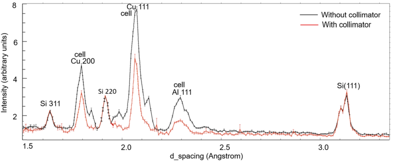
Simulated diffraction pattern of clampcell + Si with and without collimator.

Clearly, the simulated results agree very well with the experimental evaluation of the collimator. However, small discrepancies remain between the experimental and simulated results, as shown in Fig. 9 and in Fig. 10. We have identified the possible major reasons for these discrepancies as imperfections arising from the manufacturing process of the collimator, misalignment of sample and collimator and materials differences (preferred orientation, texture, precipitates) that are not accounted for in the simulation. Of these three only the materials differences could potentially cause the optimization result to differ from the experimental configuration. In future work we will investigate a more detailed model of the phases of the CuBe cell and may benefit from incorporating the texture models from McStas [20,21] to further mitigate these concerns.

The imperfections from the manufacturing process are expected to be random. Therefore though they may affect the observed peak shape, thus broadening or sharpening the minimum in optimization space, they are not expected to affect the overall result. Misalignment is somewhat different in that it is really accounting for the uncertainty with which the parts can be assembled on the beamline. However, the gauge volume studies as shown in Fig. 8, demonstrated that the diffracted result is not that sensitive to minor misalignment. Moreover as a beamline optimized for the very small samples present in high pressure experiments, SNAP is exceptionally well set-up for careful alignment procedures.

Comparing Fig. 9 and 10, the relative peak intensities are very similar. Between the simulated and experimental results, there are some differences in peak shapes that are clearly visible. Again, the majority of these features can be attributed to variations in the materials of the cell away from the ideal. A detailed analysis of the peak shape is still under study and will be presented elsewhere [13].

In conclusion, a workflow to optimize collimators for additive manufacturing has been presented. This workflow includes a McStas simulation of the incident beam in a specific beamline, MCViNE simulations of the sample, sample environment and collimator uses Mantid to reduce the results and is incorporated in a SciPy optimizer loop. The output geometry of the optimization can be converted to a .scad file for further conversion for additive manufacturing. The workflow was used to optimize a collimator for a clamp cell used on the SNAP beamline at the SNS. Such a collimator has been printed in both plastic and $B_{4} C$ and preliminary results from the plastic version were shown. Therefore, this workflow demonstrates coupling modern computational tools and modern manufacturing technologies, to make great strides in designing and deploying new, more compact collimators that can be utilized with smaller sample environments for successfully filtering the scattered beam.

Footnotes

Acknowledgements

We gratefully acknowledge J.J. Molaison for his help during the experimental evaluation on SNAP. A portion of this research used resources at the SNAP beamline of the Spallation Neutron Source, a DOE Office of Science User Facility operated by the Oak Ridge National Laboratory. The optimization constraints were determined through the expert technical efforts of D. Goldsby and D. Siddel. This work is supported by Oak Ridge National Laboratory (ORNL), Laboratory Directed Research and Development funds under contract DE-AC05-00OR8828. This research used the ORNL CADES compute resources.

References

Arnold,

J.C.

Bilheux,

J.M.

Borreguero,

Buts,

S.I.

Campbell,

Chapon,

Doucet,

Draper,

Ferraz Leal,

M.A.

Gigget al., Mantid – data analysis and visualization package for neutron scattering and

μ SR

experiments, Nuclear Instruments and Methods in Physics Research Section A: Accelerators, Spectrometers, Detectors and Associated Equipment764 (2014), 156–166. doi:10.1016/j.nima.2014.07.029.

Bertelsen, Software for simulation and design of neutron scattering instrumentation, PhD thesis, The Niels Bohr Institute, Faculty of Science, University of Copenhagen (2017).

B.J.

Bichon and

M.S.

Eldred, Efficient global surrogate modeling for reliability-based design optimization, ASME Journal of Mechanical Design107(1) (2013), 1–13.

S.-H.

Chen,

M.-C.

Chen,

P.-C.

Chang and

Mani, Multiple parents crossover operators: A new approach removes the overlapping solutions for sequencing problems, Applied Mathematical Modelling37(5) (2013), 2737–2746, https://www-sciencedirect-com.web.bisu.edu.cn/science/article/pii/S0307904X12003617 . doi:10.1016/j.apm.2012.06.005.

Coates,

H.B.

Cao,

B.C.

Chakoumakos,

M.D.

Frontzek,

Hoffmann,

A.Y.

Kovalevsky,

Liu,

Meilleur,

A.M.

dos Santos,

D.A.A.

Myles,

X.P.

Wang and

Ye, A suite-level review of the neutron single-crystal diffraction instruments at Oak Ridge National Laboratory, Review of Scientific Instruments89(9) (2018), 092802. doi:10.1063/1.5030896.

J.R.D.

Copley and

J.C.

Cook, An analysis of the effectiveness of oscillating radial collimators in neutron scattering applications, Nuclear Instruments and Methods in Physics Research Section A: Accelerators, Spectrometers, Detectors and Associated Equipment345(2) (1994), 313–323, https://www-sciencedirect-com.web.bisu.edu.cn/science/article/pii/0168900294910081 . doi:10.1016/0168-9002(94)91008-1.

Creek,

Santisteban and

Edwards, Modelling pseudo-strain effects induced in strain measurement using time-of-flight neutron diffraction (2005), http://citeseerx.ist.psu.edu/viewdoc/download?doi=10.1.1.507.6877&rep=rep1&type=pdf.

B.S.G.

de Almeida and

V.C.

Leite, Particle swarm optimization: A powerful technique for solving engineering problems, in: Swarm Intelligence, 2019, Chapter 3. doi:10.5772/intechopen.89633.

S.O.

Diallo,

J.Y.Y.

Lin,

D.L.

Abernathy and

R.T.

Azuah, Momentum and energy dependent resolution function of the ARCS neutron chopper spectrometer at high momentum transfer: Comparing simulation and experiment, Nuclear Instruments and Methods in Physics Research Section A: Accelerators, Spectrometers, Detectors and Associated Equipment835 (2016), 34–41, https://www-sciencedirect-com.web.bisu.edu.cn/science/article/pii/S0168900216308440 . doi:10.1016/j.nima.2016.08.027.

10.

Falconi,

Monaco,

W.A.

Crichton,

Mezouar and

Verbeni, Collimator for inelastic x-ray scattering experiments at high temperature and pressure conditions, High Pressure Research24(4) (2004), 463–469. doi:10.1080/08957950412331331745.

11.

García-Martínez,

F.J.

Rodriguez and

Lozano, Genetic algorithms, in: Handbook of Heuristics, 2018, pp. 431–464, ISBN 978-3-319-07124-4. doi:10.1007/978-3-319-07124-4_28.

12.

Islam, c3dp: Automated design of 3D printed collimator optimized for high pressure diffraction, Anaconda, 2019, https://github.com/Fahima-Islam/c3dp/tree/documentation.

13.

Islam,

Haberl,

Lin,

Anderson,

Molaison and

Granroth, Novel analysis method for obtaining better performance of hydrocarbon collimator, In preparation.

14.

E.B.

Iverson,

P.D.

Ferguson,

F.X.

Gallmeier and

I.I.

Popova, Detailed SNS neutronics calculations for scattering instrument design: SCT configuration, Technical report, SNS–110040300–DA0001–R00, Oak Ridge National Laboratory.

15.

Jones,

Oliphant,

Petersonet al., SciPy: Open source scientific tools for Python (2001–), http://www.scipy.org/.

16.

Kikinis,

S.D.

Pieper and

Vosburgh, 3D Slicer: A platform for subject-specific image analysis, visualization, and clinical support, in: Intraoperative Imaging Image-Guided Therapy,

F.A.

Jolesz 19, 2014, pp. 277–289, ISBN 978-1-4614-7657-3.

17.

Könnecke,

F.A.

Akeroyd,

H.J.

Bernstein,

A.S.

Brewster,

S.I.

Campbell,

Clausen,

Cottrell,

J.U.

Hoffmann,

P.R.

Jemian,

Männicke,

Osborn,

P.F.

Peterson,

Richter,

Suzuki,

Watts,

Wintersberger and

Wuttke, The NeXus data format, Journal of Applied Crystallography48(1) (2015), 301–305. doi:10.1107/S1600576714027575.

18.

Kowarik,

Bogula,

Boitano,

Carlà,

Pithan,

Schäfer,

Wilming,

Zykov and

Pithan, A novel 3D printed radial collimator for x-ray diffraction, Review of Scientific Instruments90(3) (2019), 035102. doi:10.1063/1.5063520.

19.

Laidlaw,

Trumbore and

Hughes, Constructive solid geometry for polyhedral objects, ACM Siggraph Computer Graphics20 (1986), 161–170. doi:10.1145/15922.15904.

20.

Laliena,

M.Á.

Vicente-Álvarez and

Campo, Routines for optimizing neutron scattering instruments with McStas, Technical report, 3–4, 2019.

21.

Laliena,

M.Á.

Vicente-Álvarez and

Campo, Monte Carlo simulation of neutron scattering by a textured polycrystal, Journal of Applied Crystallography53(2) (2020), 512–529. doi:10.1107/S1600576720002290.

22.

J.Y.

Lin,

H.L.

Smith,

G.E.

Granroth,

D.L.

Abernathy,

M.D.

Lumsden,

Winn,

A.A.

Aczel,

Aivazis and

Fultz, MCViNE – an object oriented Monte Carlo neutron ray tracing simulation package, Nuclear Instruments and Methods in Physics Research Section A: Accelerators, Spectrometers, Detectors and Associated Equipment810 (2016), 86–99.

23.

J.Y.Y.

Lin,

A.A.

Aczel,

D.L.

Abernathy,

S.E.

Nagler,

W.J.L.

Buyers and

G.E.

Granroth, Using Monte Carlo ray tracing simulations to model the quantum harmonic oscillator modes observed in uranium nitride, Physical Review B89(14) (2014), 144302.

24.

J.Y.Y.

Lin,

Islam,

Sala,

Lumsden,

Smith,

Doucet,

M.B.

Stone,

D.L.

Abernathy,

Ehlers,

J.F.

Ankner and

G.E.

Granroth, Recent developments of MCViNE and its applications at SNS, Journal of Physics Communications3(8) (2019), 085005. doi:10.1088/2399-6528/ab3622.

25.

Lu, Moderator performance of the SNS as-built configuration, Technical report, SNS–106100200–TR0199–R00, Oak Ridge National Laboratory.

26.

Lu,

Gallmeier,

Ferguson,

Iverson and

Popova, Improved moderator performance calculations at SNS, in: Tenth International Topical Meeting on Nuclear Applications of Accelerators (AccApp11), 2011.

27.

T.E.

Mason,

Abernathy,

Anderson,

Ankner,

Egami,

Ehlers,

Ekkebus,

Granroth,

Hagen,

Herwig,

Hodges,

Hoffmann,

Horak,

Horton,

Klose,

Larese,

Mesecar,

Myles,

Neuefeind,

Ohl,

Tulk,

X.-L.

Wang and

Zhao, The spallation neutron source in Oak Ridge: A powerful tool for materials research, Physica B: Condensed Matter385 (2006), 955–960. doi:10.1016/j.physb.2006.05.281.

28.

Mauws,

A.M.

Hallas,

Sala,

A.A.

Aczel,

P.M.

Sarte,

Gaudet,

Ziat,

J.A.

Quilliam,

J.A.

Lussier,

Bieringer,

H.D.

Zhou,

Wildes,

M.B.

Stone,

Abernathy,

G.M.

Luke,

B.D.

Gaulin and

C.R.

Wiebe, Dipolar-octupolar Ising antiferromagnetism in

{Sm}_{2} {Ti}_{2} O_{7}

: A moment fragmentation candidate, Phys. Rev. B98 (2018), 100401. doi:10.1103/PhysRevB.98.100401.

29.

Morard,

Mezouar,

Bauchau,

Álvarez-Murga,

J.-L.

Hodeau and

Garbarino, High efficiency multichannel collimator for structural studies of liquids and low-Z materials at high pressures and temperatures, Review of Scientific Instruments82(2) (2011), 023904. doi:10.1063/1.3551988.

30.

J.L.

Niedziela,

Mills,

M.J.

Loguillo,

H.D.

Skorpenske,

Armitage,

H.L.

Smith,

J.Y.Y.

Lin,

M.S.

Lucas,

M.B.

Stone and

D.L.

Abernathy, Design and operating characteristic of a vacuum furnace for time-of-flight inelastic neutron scattering measurements, Review of Scientific Instruments88(10) (2017), 105116. doi:10.1063/1.5007089.

31.

Pawlik and

Ozga , LaboTex: The texture analysis software (1999).

32.

Podlesnyak,

Loguillo,

G.M.

Rucker,

Haberl,

Boehler,

Ehlers and

L.L.

Daemen, Clamp cell with in-situ pressure monitoring for low-temperature neutron scattering measurements, High Pressure Research38(4) (2018), 482–492. doi:10.1080/08957959.2018.1519560.

33.

T.R.

Prisk,

M.S.

Bryan,

P.E.

Sokol,

G.E.

Granroth,

Moroni and

Boninsegni, The momentum distribution of liquid

^{4} He

, Journal of Low Temperature Physics (2017). doi:10.1007/s10909-017-1798-7.

34.

C.J.

Ridley,

Manuel,

Khalyavin,

Kirichek and

K.V.

Kamenev, A novel compact three-dimensional laser-sintered collimator for neutron scattering, Review of Scientific Instruments86(9) (2015), 095114. doi:10.1063/1.4931695.

35.

Wikipedia contributors, OpenSCAD – Wikipedia, the free encyclopedia (2019), [Online; accessed 11-November-2019].

36.

P.K.

Willendrup and

Lefmann, McStas (i): Introduction, use, and basic principles for ray-tracing simulations, Journal of Neutron Research22(1) (2020), 1–16. doi:10.3233/JNR-190108.

37.

Yiu,

A.A.

Aczel,

G.E.

Granroth,

D.L.

Abernathy,

M.B.

Stone,

W.J.L.

Buyers,

J.Y.Y.

Lin,

G.D.

Samolyuk,

G.M.

Stocks and

S.E.

Nagler, Light atom quantum oscillations in UC and US, Physical Review B93(1) (2016), 014306.