The effect of ruralness on vocational rehabilitation applications

Abstract

BACKGROUND:

Most of the literature on evaluating vocational rehabilitation (VR) programs has taken application to the VR program as given despite the obvious selection issues associated with the decision to apply.

OBJECTIVE:

In this paper, we focus on the decision to apply for VR services and, in particular, on the effect of ruralness on that decision.

METHODS:

We use ordinary least squares with and without state-specific fixed effects along with maximum likelihood estimation (MLE) to estimate models of the application decision.

RESULTS:

We find that people with disabilities from rural counties are less likely to apply for VR services than people with disabilities in more urban counties. We also find a wide distribution in state-specific fixed effect MLE estimates and show that only a small part of the variation across states is due to variation in Order-of-Selection rules.

CONCLUSIONS:

We conclude that states should sponsor more research to better understand variation in VR application rates across states and across counties. We also suggest how such research could be used to raise low application rates.

Keywords

Rural vocational rehabilitation maximum likelihood estimation (MLE)

1 Introduction

The Rehabilitation Services Administration (RSA) provides formula-based grants to Vocational Rehabilitation (VR) agencies to improve the employment outcomes of people with disabilities. Eighty VR agencies located in all US states, Washington DC, and territories offer a consistent menu of services based on individualized needs. Services for eligible individuals with disabilities may include vocational assessment, counseling and guidance, information and referral, physical and mental restoration, training and education, job search, job placement, job coaching, and supported employment (United States Department of Disability Services, n.d.).

Each VR agency has some autonomy in how it organizes, delivers, and pays for services. For instance, 23 states operate both blind and general agencies, while the remaining 27 states operate combined agencies. Together, the state-federal VR system invests approximately $4 billion dollars annually to help people with disabilities prepare for, secure, or maintain employment (United States Department of Disability Services, n.d.).

One data source for evaluating VR performance across various programs is the RSA-911 data. Historically, RSA-911 data has included individual consumer characteristics, services provided, and employment outcomes for VR cases closed each year. Researchers and program evaluators have used the RSA-911 data system extensively to examine productivity across agencies, outcomes for different disability and demographic groups, and other service factors (e.g. Honeycutt et al., 2017; Ipsen & Swicegood, 2015, 2017; Kaya et al., 2016; Langi & Balcazar, 2017). For instance, Langi and Balcazar (2017) found that being non-white increased the risk of being denied eligibility into the VR program and not receiving services if deemed eligible.

Starting in 2014, RSA-911 case data included county and ZIP code information. The addition of these variables allowed researchers to examine cases in additional ways, such as based on rural and urban location or controlling for economic variation across place. Ipsen and Swicegood (2015) found that case mix and employment outcomes varied significantly across geography. They reported that the rural case mix had higher rates of people with physical and learning disabilities, while the urban case mix had higher rates of people with mental illness. Rural case mix was also younger, while urban case mix was more educated and had higher rates of minority applicants. Employment outcomes varied across place as well. Rural locations had higher rates of employment and self-employment outcomes, while urban locations had higher rates of employment with supports in integrated settings.

These types of findings lead to additional questions and hypotheses about the reasons for geographic variation. While past research has described how case outcomes differ once VR clients apply for VR services, this paper explores whether potential VR consumers are recruited or apply for services at similar rates across place. If systematic variations occur, this provides a strong signal to VR programs about the effectiveness of their outreach and delivery strategies.

On a methodological note, almost all of the treatment effects literature ignores the selection effects associated with applying to a program (see, for example, Aakvik et al., 2005; Heckman et al., 1999; Imbens & Wooldridge, 2009). Usually, this stems from a lack of data on the pool of potential applicants, making it difficult to infer anything about selection. Recent exceptions include Dean et al. (2017, 2019) and Hamilton et al. (2018). In all three cases, the authors had available data on the pool of potential applicants. In this paper, we focus on the decision to apply, which would be the first step in a two-step approach, similar to Heckman (1979), to measure the effects of receiving VR services. We use estimated data from the American Community Survey (ACS) to develop a proxy for the potential applicant pool by counting people with disabilities in each county based on a “yes” response to one of six functional limitation questions.

1.1 Variation in VR application rates

Rates of VR applications may differ based on perceived expected benefit and other characteristics of services. From a geographic perspective, one might expect different rates of VR applications based on sociodemographic need. Data from the ACS show higher rates of disability, higher rates of poverty, and lower rates of employment among people with disabilities age 18–65 living in micro and noncore counties, relative to metropolitan counties (ACS, Table S1810; ACS, Table C18130; ACS, Table C18120). Based on increased need and opportunity to receive the full complement of VR services, one might anticipate VR would have higher rates of rural applications.

Alternately, there is evidence that the quality of VR services may be lower in rural communities, and application rates may reflect this based on perceived quality. Perceptions of benefit stem from a variety of factors including employment barriers and VR outreach efforts. There is evidence that VR service quality may be lower in rural areas due to slower delivery pacing and fewer VR counselor and provider contacts with consumers (Ipsen et al., 2012, 2019; Rigles et al., 2011). Reinforcing these findings, Rigles et al. (2011) reported high rates of premature exit from the VR system for rural consumers due to “refused service” and “failure to cooperate” reasons.

Geographic difference may also be related to perceived ability to benefit from services and secure employment. Rates of “out of the labor force” for people with disabilities increases from metro (58%), to micro (62%), to noncore (65%) (ACS, Table C18120). Dropping out of the labor force may imply discouragement about securing employment. Additional employment barriers, such as limited access to transportation options (Ipsen, 2012; McDaniels et al., 2018), lower educational attainment (Erickson et al., 2018), and limited economic choices may reinforce a reluctance to seek services.

There is significant literature that shows that transportation availability is critical for employment (Arkansas Research and Training Center on Vocational Rehabilitation, 1992; Bearse et al., 2004; Clapp, Stern, and Yu, 2019; Ipsen, 2012; Jolly, Priestley, and Matthews, 2006; McDaniels, Harley, and Beach, 2018; National Council on Disability, 2005; Sabella, Bezyak, and Gattis, 2016; Stern, 1993; West et al., 1998), and that rural areas have less developed transportation systems (Clapp, Stern, and Yu, 2019; Mattson, 2015).

It is also likely that VR agencies do not conduct consistent outreach across locations. Many rural communities lack central access points for reaching eligible VR consumers and VR programs allocate uneven resources across place to conduct community outreach activities (Ysasi et al., 2018).

1.2 Data

To explore geographic variation in VR applications, we calculated VR recruitment rates for metro, micro, and noncore counties in each state for general and combined VR agencies (n = 51). We excluded VR agencies dedicated to serving the blind and low vision population (n = 23) due to the limited number of consumers served in these agencies and recruitment strategies that are very targeted to a specific population and might impact application rates.

We used two datasets to develop VR application rates, including the 2015 RSA-911 case services file and the 2013–2017 American Community Survey (ACS) 5-year summary file (S1810). ACS data are aggregated as they are collected and released in 1-, 3-, and 5-year estimates. For rural areas, data are aggregated across 5 years to protect confidentiality and achieve a suitable sample size for reliable estimates.

The ACS collects data on a variety of demographic variables. To measure the disability population, the ACS includes six questions related to functional limitation focused on hearing, vision, cognitive, ambulatory, self-care, and independent living difficulties. Any person who answers “yes” to one or more of the functional limitation questions is counted in the disability population. We use this estimate as a proxy for the pool of potential applicants to the VR system but acknowledge evidence that some disability groups may be underrepresented, including those with learning and intellectual disabilities and mental illness (Hall et al., 2012; Henderson, 2011).

For both files, we used county-level Federal Information Processing System (FIPS) codes to classify counties as metro, micro, or noncore using an Office of Management and Budget (OMB) rural-urban classification. The OMB classifications assign metropolitan (metro) status to counties that contain an urban core of at least 50,000 people or if a significant proportion of the population commutes into an adjacent urban core. Non-metro counties are classified into micropolitan (micro) and noncore counties, where micro counties have an urban core of 10,000 to 50,000 people and noncore counties do not. Although metro, micro, and noncore designations do not fully describe the varied conditions across place, they provide a common rubric for exploring rural-urban differences. Similar methods have been used to explore variation in describing VR service delivery across place (Ipsen & Swicegood, 2015, 2017).

To calculate the number of metro, micro, and noncore VR applications for each state, we first aggregated cases across each county and then aggregated the number of county applications based on metro, micro, and noncore county designations. We made similar calculations using ACS data to calculate the total number of people with disabilities residing in each state’s metro, micro, and noncore counties, based on a “yes” answer to any one of the six ACS disability questions. Using these two estimates, we calculated metro, micro, and noncore application rates for each state’s general or combined VR agency. Table 1 shows the raw data used to make application estimates across geography. While a few exceptions exist, recruitment rates are lower in noncore counties relative to metro counties.

Table 1
Raw data

# Applicants to VR Agency Estimated # people w/Disabilities Proportion of people w/ Disabilities who applied for VR services

State Noncore Micro Metro Noncore Micro Metro Noncore Micro Metro

Alabama 386 487 5,775 48,194 65,236 304,741 0.008 0.007 0.019

Alaska 186 231 1,232 13,185 3,004 31,595 0.014 0.077 0.039

Arizona 34 258 4,576 7,624 19,104 388,259 0.004 0.014 0.012

Arkansas 703 982 2,211 59,662 62,175 145,834 0.012 0.016 0.015

California 182 811 34,300 21,941 51,165 1,922,180 0.008 0.016 0.018

Colorado 253 394 3,833 22,614 18,714 256,040 0.011 0.021 0.015

Connecticut 0 150 3,261 0 9,112 177,846 0.016 0.018

Delaware 0 0 2,899 0 0 55,236 0.052

DC 0 0 60 0 0 45,190 0.001

Florida 361 247 20,919 30,551 25,497 1,152,005 0.012 0.010 0.018

Georgia 227 569 3,571 69,546 81,737 518,685 0.003 0.007 0.007

Hawaii 0 395 1,002 0 13,688 51,090 0.029 0.020

Idaho 253 633 3,220 11,895 26,248 72,956 0.021 0.024 0.044

Illinois 698 1,166 10,425 45,266 60,012 575,400 0.015 0.019 0.018

Indiana 402 1,341 5,452 36,554 78,575 362,086 0.011 0.017 0.015

Iowa 648 861 2,147 40,233 36,010 99,112 0.016 0.024 0.022

Kansas 501 577 2,893 28,408 37,607 118,980 0.018 0.015 0.024

Kentucky 1,368 1,059 5,110 126,906 92,150 206,464 0.011 0.011 0.025

Louisiana 148 167 5,088 27,643 38,003 301,833 0.005 0.004 0.017

Maine 1,061 666 1,895 41,195 10,598 58,922 0.026 0.063 0.032

Maryland 71 74 5,585 5,896 4,321 312,701 0.012 0.017 0.018

Massachusetts 5 398 9,867 570 5,724 383,156 0.009 0.070 0.026

Michigan 480 1,158 11,678 62,701 83,387 602,028 0.008 0.014 0.019

Minnesota 304 678 4,367 30,636 39,640 221,664 0.010 0.017 0.020

Mississippi 759 1,745 2,170 66,882 86,506 106,962 0.011 0.020 0.020

Missouri 1,258 927 7,887 84,902 65,785 312,769 0.015 0.014 0.025

Montana 616 329 1,599 26,423 19,350 24,536 0.023 0.017 0.065

Nebraska 580 521 2,551 18,430 19,347 66,762 0.031 0.027 0.038

Nevada 52 214 2,325 2,193 20,383 172,037 0.024 0.010 0.014

New Hampshire 169 1,734 1,323 3,758 31,955 48,227 0.045 0.054 0.027

New Jersey 0 0 10,199 0 0 431,402 0.024

New Mexico 116 910 2,262 8,123 52,376 99,272 0.014 0.017 0.023

New York 707 1,827 25,490 30,383 76,568 984,340 0.023 0.024 0.026

North Carolina 1,032 2,658 9,913 58,463 138,252 508,239 0.018 0.019 0.020

North Dakota 125 294 645 10,892 8,958 18,666 0.011 0.033 0.035

Ohio 222 2,156 12,385 38,335 152,082 644,235 0.006 0.014 0.019

Oklahoma 877 1,250 3,807 55,205 64,380 205,056 0.016 0.019 0.019

Oregon 136 846 4,855 9,121 51,493 241,698 0.015 0.016 0.020

Pennsylvania 434 1,890 15,008 31,001 87,469 750,565 0.014 0.022 0.020

Puerto Rico 0 1 1 783 15,689 352,998 0.000 0.000 0.000

Rhode Island 0 0 1,717 0 0 72,389 0.024

South Carolina 783 1,239 8,103 31,161 39,194 301,723 0.025 0.032 0.027

South Dakota 204 311 468 13,703 13,955 24,024 0.015 0.022 0.019

Tennessee 227 386 4,213 66,888 87,588 391,211 0.003 0.004 0.011

Texas 1,203 1,595 23,166 110,816 120,064 1,382,242 0.011 0.013 0.017

Utah 515 591 7,742 9,515 8,713 131,794 0.054 0.068 0.059

Vermont 1,541 1,408 1,039 13,497 18,999 13,742 0.114 0.074 0.076

Virginia 548 256 4,022 64,425 29,664 386,357 0.009 0.009 0.010

Washington 226 597 7,975 14,418 47,555 417,282 0.016 0.013 0.019

West Virginia 1,256 813 2,430 46,206 33,585 111,308 0.027 0.024 0.022

Wisconsin 613 1,263 8,726 48,968 47,517 248,287 0.013 0.027 0.035

Wyoming 283 826 623 9,914 16,083 12,701 0.029 0.051 0.049

	# Applicants to VR Agency	Estimated # people w/Disabilities	Proportion of people w/ Disabilities who applied for VR services
Alabama	386	487	5,775	48,194	65,236	304,741	0.008	0.007	0.019
Alaska	186	231	1,232	13,185	3,004	31,595	0.014	0.077	0.039
Arizona	34	258	4,576	7,624	19,104	388,259	0.004	0.014	0.012
Arkansas	703	982	2,211	59,662	62,175	145,834	0.012	0.016	0.015
California	182	811	34,300	21,941	51,165	1,922,180	0.008	0.016	0.018
Colorado	253	394	3,833	22,614	18,714	256,040	0.011	0.021	0.015
Connecticut	0	150	3,261	0	9,112	177,846	0.016	0.018
Delaware	0	0	2,899	0	0	55,236	0.052
DC	0	0	60	0	0	45,190	0.001
Florida	361	247	20,919	30,551	25,497	1,152,005	0.012	0.010	0.018
Georgia	227	569	3,571	69,546	81,737	518,685	0.003	0.007	0.007
Hawaii	0	395	1,002	0	13,688	51,090	0.029	0.020
Idaho	253	633	3,220	11,895	26,248	72,956	0.021	0.024	0.044
Illinois	698	1,166	10,425	45,266	60,012	575,400	0.015	0.019	0.018
Indiana	402	1,341	5,452	36,554	78,575	362,086	0.011	0.017	0.015
Iowa	648	861	2,147	40,233	36,010	99,112	0.016	0.024	0.022
Kansas	501	577	2,893	28,408	37,607	118,980	0.018	0.015	0.024
Kentucky	1,368	1,059	5,110	126,906	92,150	206,464	0.011	0.011	0.025
Louisiana	148	167	5,088	27,643	38,003	301,833	0.005	0.004	0.017
Maine	1,061	666	1,895	41,195	10,598	58,922	0.026	0.063	0.032
Maryland	71	74	5,585	5,896	4,321	312,701	0.012	0.017	0.018
Massachusetts	5	398	9,867	570	5,724	383,156	0.009	0.070	0.026
Michigan	480	1,158	11,678	62,701	83,387	602,028	0.008	0.014	0.019
Minnesota	304	678	4,367	30,636	39,640	221,664	0.010	0.017	0.020
Mississippi	759	1,745	2,170	66,882	86,506	106,962	0.011	0.020	0.020
Missouri	1,258	927	7,887	84,902	65,785	312,769	0.015	0.014	0.025
Montana	616	329	1,599	26,423	19,350	24,536	0.023	0.017	0.065
Nebraska	580	521	2,551	18,430	19,347	66,762	0.031	0.027	0.038
Nevada	52	214	2,325	2,193	20,383	172,037	0.024	0.010	0.014
New Hampshire	169	1,734	1,323	3,758	31,955	48,227	0.045	0.054	0.027
New Jersey	0	0	10,199	0	0	431,402	0.024
New Mexico	116	910	2,262	8,123	52,376	99,272	0.014	0.017	0.023
New York	707	1,827	25,490	30,383	76,568	984,340	0.023	0.024	0.026
North Carolina	1,032	2,658	9,913	58,463	138,252	508,239	0.018	0.019	0.020
North Dakota	125	294	645	10,892	8,958	18,666	0.011	0.033	0.035
Ohio	222	2,156	12,385	38,335	152,082	644,235	0.006	0.014	0.019
Oklahoma	877	1,250	3,807	55,205	64,380	205,056	0.016	0.019	0.019
Oregon	136	846	4,855	9,121	51,493	241,698	0.015	0.016	0.020
Pennsylvania	434	1,890	15,008	31,001	87,469	750,565	0.014	0.022	0.020
Puerto Rico	0	1	1	783	15,689	352,998	0.000	0.000	0.000
Rhode Island	0	0	1,717	0	0	72,389	0.024
South Carolina	783	1,239	8,103	31,161	39,194	301,723	0.025	0.032	0.027
South Dakota	204	311	468	13,703	13,955	24,024	0.015	0.022	0.019
Tennessee	227	386	4,213	66,888	87,588	391,211	0.003	0.004	0.011
Texas	1,203	1,595	23,166	110,816	120,064	1,382,242	0.011	0.013	0.017
Utah	515	591	7,742	9,515	8,713	131,794	0.054	0.068	0.059
Vermont	1,541	1,408	1,039	13,497	18,999	13,742	0.114	0.074	0.076
Virginia	548	256	4,022	64,425	29,664	386,357	0.009	0.009	0.010
Washington	226	597	7,975	14,418	47,555	417,282	0.016	0.013	0.019
West Virginia	1,256	813	2,430	46,206	33,585	111,308	0.027	0.024	0.022
Wisconsin	613	1,263	8,726	48,968	47,517	248,287	0.013	0.027	0.035
Wyoming	283	826	623	9,914	16,083	12,701	0.029	0.051	0.049

For the statistical analyses presented, we weight the data presented in the last three columns of Table 1 by the number of people with disabilities (in the middle three columns of Table 1). We do this because each person represented makes an individual decision about whether to apply for VR services. Using the weights in ordinary least squares (OLS) or maximum likelihood estimation (MLE) is equivalent to performing the chosen econometric method using data on the individual people with disabilities. Appendix A discusses weighting issues in more detail.

2 Methodology

We estimate three equations. The first two are linear equations with dependent variables log(y_ij) where y_ij is the proportion of people with disabilities in type j counties from state i that apply for VR services. 1 Explanatory variables for the first equation are binary variables for each county type (i.e., noncore, micro, and metro counties. In the second equation, one of the county type variables is replaced with 52 state-specific binary variables 2 (state-specific fixed effects).

The first model is estimated with Ordinary Least Squares (OLS), and the second by differencing the data within each state from the state average and then using OLS. In both of these equations, there is an issue about assumed degrees of freedom. This issue is explained in detail in the discussion of Maximum Likelihood Estimation (MLE) in Appendix B.

The third model is more structural and is estimated using MLE. Define $y_{ijk}^{*}$ as the net benefit for person k, k = 1, 2,..,K_ij, living in a type j county (noncore, micro, or metro), j = 1, 2,..,J, in state i, i = 1, 2,..,n, of applying for VR services with $\begin{matrix} y_{ijk}^{*} = β_{i} + 1 (j < J) α_{j} + δ u_{ij} + ɛ_{ijk}, \\ u_{ij} \sim iidN (0, 1), \\ ɛ_{ijk} \sim iidN (0, 1) . \end{matrix}$ (1)

The β terms are state-specific (fixed) effects, and the α terms are county type binary variables for noncore and micro county types. The δu_ij error terms are state/county type-specific unobserved heterogeneity with standard deviation δ, and the ɛ_ijk errors are person-specific, idiosyncratic errors. 3

3 Estimation results

3.1 OLS estimates

We first report results for the log-linear models described in section 3. Table 2 presents estimates of the county-type effects when not controlling for state-specific fixed effects. All three estimates are very precisely estimated despite only 8.7% of the data variation being explained by the equation. The estimates increase in value as counties move from noncore to micro to metro and imply application rates of 1.18% for noncore counties, 1.52% for micro counties, and 1.86% for metro counties. 4 According to these estimates, people with disabilities living in metro counties are 57% more likely to apply for VR services than are people with disabilities in noncore counties.

Table 2
OLS estimates in levels without state specific effects

Variable Estimate Std Err t-Statistic

Noncore –4.9439^ 0.001 –7,394.600

Micro –4.186^ 0.001 –8,193.000

Metro –3.987^** 0.000 –21,276.300

Variable	Estimate	Std Err	t-Statistic
Noncore	–4.9439^**	0.001	–7,394.600
Micro	–4.186^**	0.001	–8,193.000
Metro	–3.987^**	0.000	–21,276.300

Notes: 1) R² = 0.087. 2) Double-starred items are statistically significant at the 1% level. 3) The estimate of the standard deviation of the error is 0.424.

Table 3 shows the effect on the county-type effects of including state-specific fixed effects. The order-of-magnitude change in the size of the parameters is not meaningful. In Table 2, the estimates include mean state-specific effects (because state-specific effects were not included). On the other hand, Table 3 differences out the state-specific effects. Thus, the relevant comparison is the differences in the estimates across the two tables.

Table 3

OLS estimates in levels with state-specific effects

Variable	Estimate	Std Err	t-Statistic
Noncore	–0.511^**	0.000	–2,001.5
Micro	–0.218^**	0.000	–994.0

Notes: 1) R² = 0.492. 2) Double-starred items are statistically significant at the 1% level. 3) The estimate of the standard deviation of the error is 0.143.

The three analogous estimates in Table 3 are 0.000, 5 –0.218, and –0.511 for metro, micro, and noncore counties respectively. The corresponding estimates from Table 2 are –3.987, –4.186, and –4.439. The two sets of estimates are not that different in terms of their differences suggesting that the state-specific effect has only a small correlation with the county type log application rates from the state. 6

The estimate of the standard deviation of the error decreases from 0.424 in Table 2 to 0.143 in Table 3. This occurs because of the addition of 47 state-specific fixed effects. 7 The estimate from Table 3 is a more useful number for making statements about variation across counties in VR application rates.

Table 4 presents the estimates of the fixed effects. 8 Some states are excluded from the table because there was no variation in county type within the state. 9

Table 4

Estimated Fixed Effects

State	Estimate	State	Estimate
Alabama	–2.989	Montana	–1.949
Alaska	–1.785	Nebraska	–1.874
Arizona	–3.144	Nevada	–2.629
Arkansas	–2.686	New Hampshire	–1.632
California	–2.748	New Jersey	Excluded
Colorado	–2.611	New Mexico	–2.454
Connecticut	–1.950	New York	–2.143
Delaware	Excluded	North Carolina	–2.403
DC	Excluded	North Dakota	–2.177
Florida	–2.788	Ohio	–2.880
Georgia	–3.645	Oklahoma	–2.451
Hawaii	–1.635	Oregon	–2.503
Idaho	–1.993	Pennsylvania	–2.433
Illinois	–2.470	Puerto Rico	Excluded
Indiana	–2.685	Rhode Island	Excluded
Iowa	–2.326	South Carolina	–2.013
Kansas	–2.407	South Dakota	–2.410
Kentucky	–2.658	Tennessee	–3.641
Louisiana	–3.337	Texas	–2.736
Maine	–1.715	Utah	–1.242
Maryland	–2.599	Vermont	–0.879
Massachusetts	–2.113	Virginia	–3.124
Michigan	–2.790	Washington	–2.590
Minnesota	–2.632	West Virginia	–2.145
Mississippi	–2.522	Wisconsin	–2.214
Missouri	–2.480	Wyoming	–1.608

3.2 Maximum likelihood estimates

On the one hand, there is no model of individual behavior that aggregates up to the OLS model. On the other, the model of individual behavior for MLE is explicitly specified and aggregates appropriately. Also, the maximum likelihood estimates are consistent and efficient (to the degree that the simulated log likelihood contributions are precisely evaluated).

Tables 5 and 6 present the MLE estimates. First, in Table 5, we see the estimates of the parameters other than the state-specific fixed effects. The estimates are not directly comparable to those in Table 3. The three estimates in Table 3 are 0.000, –0.218, and –0.511 for metro, micro, and noncore counties respectively. In Table 5, they are 0.000, –0.066, and –0.176. Part of the difference in the estimates is that the estimates in Table 3 should be interpreted as the change in the expected value of the log of the probability of application due to a change in the county type, while the estimates in Table 5 should be interpreted as the change in the value of applying for VR services $y_{ijk}^{*}$ due to a change in the county type. 10

Table 5
MSL Estimates Other than State-Specific Fixed Effects

Estimate Std Err

Noncore –0.176^ 0.0005

Micro –0.066^ 0.0003

Delta 0.0004 0.0089

	Estimate	Std Err
Noncore	–0.176^**	0.0005
Micro	–0.066^**	0.0003
Delta	0.0004	0.0089

Note: Double-starred items are statistically significant at the 1% level.

The other key result from Table 5 is the estimate of δ (Delta) from equation (1), the standard deviation of the unobserved heterogeneity. The very small value supports the argument that there are no important state-specific/county-type effects and that it is reasonable to think of each person with a disability behaving independently of other people with disabilities in counties of the same type.

In much of the literature, researchers report average marginal effects implied by the parameter estimates. In this particular application, it is quite simple to construct marginal effects. These are presented in Fig. 1. It displays the distribution of estimated VR application rates across states and by county type using the estimates from Tables 5 and 6. 11

Table 6

MSL Estimates of State-Specific Fixed Effects

State	Estimate	State	Estimate
Alabama	–2.120^**	Montana	–1.721^**
Alaska	–1.772^**	Nebraska	–1.773^**
Arizona	–2.260^**	Nevada	–2.209^**
Arkansas	–2.131^**	New Hampshire	–1.735^**
California	–2.102^**	New Jersey	–1.985^**
Colorado	–2.152^**	New Mexico	–2.013^**
Connecticut	–2.089^**	New York	–1.940^**
Delaware	–1.621^**	North Carolina	–2.043^**
DC	–3.011^**	North Dakota	–1.858^**
Florida	–2.095^**	Ohio	–2.087^**
Georgia	–2.459^**	Oklahoma	–2.051^**
Hawaii	–2.008^**	Oregon	–2.053^**
Idaho	–1.757^**	Pennsylvania	–2.043^**
Illinois	–2.080^**	Puerto Rico	–3.633^**
Indiana	–2.145^**	Rhode Island	–1.983^**
Iowa	–1.987^**	South Carolina	–1.903^**
Kansas	–1.988^**	South Dakota	–2.014^**
Kentucky	–2.043^**	Tennessee	–2.344^**
Louisiana	–2.160^**	Texas	–2.126^**
Maine	–1.775^**	Utah	–1.550^**
Maryland	–2.098^**	Vermont	–1.285^**
Massachusetts	–1.935^**	Virginia	–2.301^**
Michigan	–2.082^**	Washington	–2.078^**
Minnesota	–2.066^**	West Virginia	–1.934^**
Mississippi	–2.036^**	Wisconsin	–1.841^**
Missouri	–1.983^**	Wyoming	–1.629^**

Note: Double-starred items are statistically significant at the 1% level.

Fig. 1

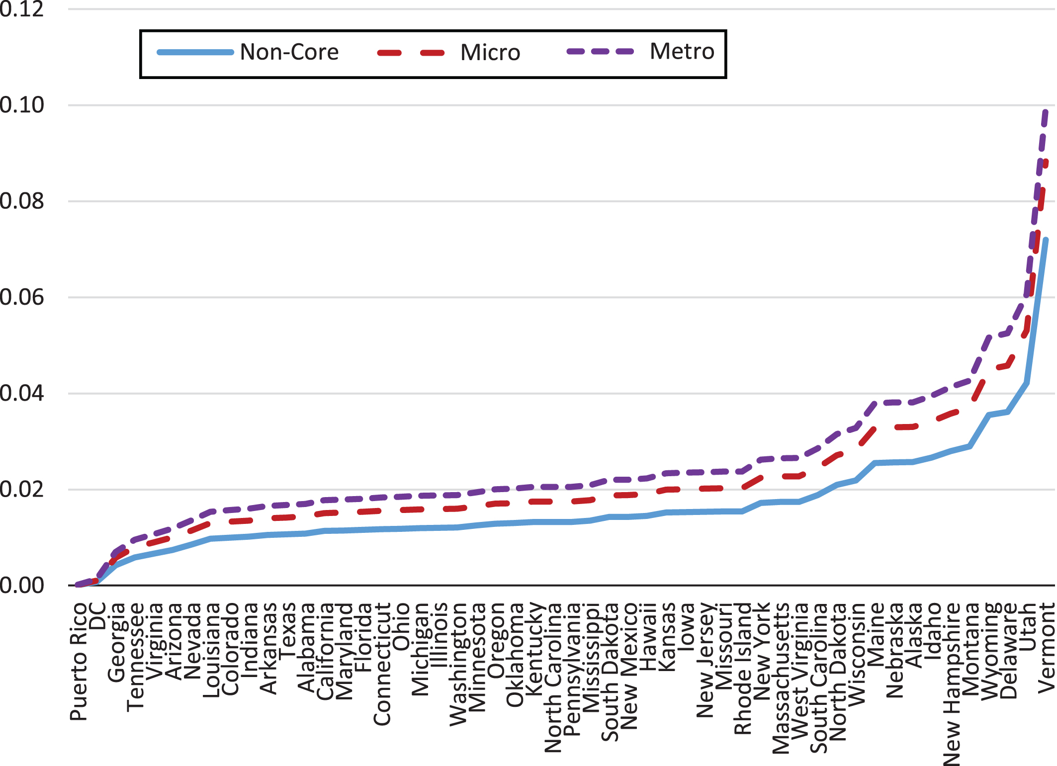
Estimated VR Application Rates.

One sees in Table 5 that metro counties dominate micro counties which, in turn, dominate noncore counties. However, it is also clear from comparing the estimates in Table 5 to those in Table 6 12 that the variation across county types within a state is much smaller than the variation across states conditional on county type. However, both types of variation are important.

Part of the variation across states might be caused by variation in whether each state is under an Order of Selection (OOS) regime. 13 OOS occurs when a VR agency receives more eligible applicants than its budget can accommodate. In these situations, applicants are ranked based on disability severity, and those with the most significant disabilities are served first. However, in 2015, there were 20 states under OOS that appeared not to be binding in the sense that the size of the state VR agency’s OOS waiting list was less than 5% of the number of applicants.

Thus, we created a new variable, called “modified OOS” equal to 1 if and only if the state was under an OOS and the size of the waiting list was at least 5% of the number of applicants. Table 7 shows which states were not under OOS, which ones are under non-binding OOS (wait list is < 5% of number of applicants), and which ones are under binding OOS (wait list is ≥ 5% of number of applicants).

Table 7

Order-of-Selection and Modified Order-of-Selection by State

	OOS	Modified OOS		OOS	Modified OOS
Alabama	No	No	Montana	Yes	No
Alaska	No	No	Nebraska	No	No
Arizona	Yes	Yes	Nevada	No	No
Arkansas	No	No	New Hampshire	No	No
California	Yes	No	New Jersey	Yes	No
Colorado	Yes	Yes	New Mexico	Yes	No
Connecticut	No	No	New York	No	No
DC	No	No	North Carolina	No	No
Delaware	Yes	No	North Dakota	Yes	No
Florida	Yes	Yes	Ohio	No	No
Georgia	Yes	No	Oklahoma	Yes	No
Hawaii	Yes	No	Oregon	No	No
Idaho	No	No	Pennsylvania	Yes	No
Illinois	Yes	No	Puerto Rico	No	No
Indiana	No	No	Rhode Island	Yes	No
Iowa	Yes	Yes	South Carolina	No	No
Kansas	Yes	No	South Dakota	Yes	No
Kentucky	Yes	No	Tennessee	Yes	Yes
Louisiana	Yes	No	Texas	No	No
Maine	No	No	Utah	Yes	Yes
Maryland	Yes	Yes	Vermont	Yes	No
Massachusetts	No	No	Virginia	Yes	Yes
Michigan	No	No	Washington	No	No
Minnesota	Yes	Yes	West Virginia	Yes	Yes
Mississippi	No	No	Wisconsin	Yes	Yes
Missouri	Yes	No	Wyoming	No	No

Notes: 1) States in darker shaded are under both order-of-selection and modified order-of-selection. 2) Shades states are under order-of-selection but not modified order-of-selection. 3) Remaining states are not under order-of-selection.

Figure 2 shows the distribution of MLEs of the state-specific fixed effects (from Table 6). 14 For example, the median (0.5 on the vertical axis) value of the modified OOS states is –2.096, and the median value for not modified OOS states is –2.035. Similarly, 20% of modified OOS states have state-specific fixed effect estimates that are greater than –1.94, and 20% of the not modified OOS states have estimates greater than –1.78. In general, since the distribution curve for not modified OOS states is to the right of the curve for modified OOS states (stochastic domination), the not modified OOS states have bigger state-specific estimates on average and at any quantile of the distributions. The average difference (not modified OOS minus modified OOS) between the two distributions (evaluated at every decile between 0.1 and 0.9) is 0.126. This implies that the existence of OOS regimes explains 0.126 of the difference in state fixed effects from Table 6. While this is a meaningful effect, it is only moderate in size. For example, it would move Virginia from –2.301 to –2.175 which would still be large.

Fig. 2

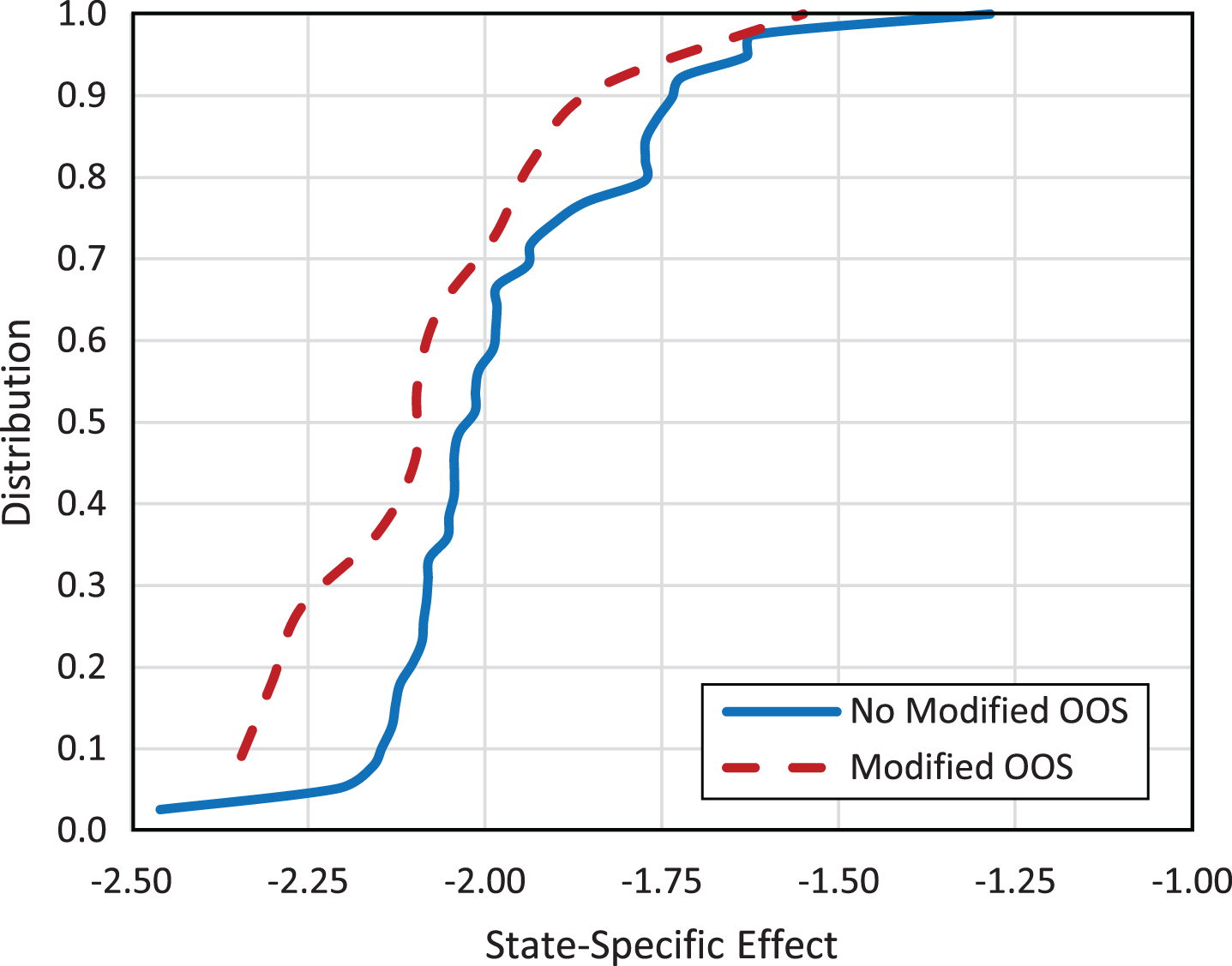
Distribution of MLEs of State-Specific Effects Disaggregated by Modified OOS.

4 Data considerations

Our models and, in particular, the MLE model and estimates provide a straightforward and easily replicable way to evaluate VR application rates across geography. Dean et al. (2017, 2019) estimate similar models for people with mental illness in Virginia (2017) and transitioning youth in Virginia (2019) as part of an attempt to control for selection bias associated with applying for VR services. The method of estimating the number of people with mental illness by county in Dean et al. (2017) is quite different than ours, but the authors can measure the effect of individual characteristics on the propensity to apply for VR services. They find that being female, white, single, a veteran, a high school dropout, in poor health with ADL and IADL problems each increase the probability of applying for VR services. Also, more to the point, they find that living in an MSA increases y^*, the value of applying, by a small but statistically significant amount (0.09). Dean et al. (2019) use a method more like ours in that they use estimates (from state administrative data) on the number of transitioning youths in each county disaggregated by disability type. On the one hand, Dean et al. (2017, 2019) can control for individual characteristics, while we do not have the data to do so. On the other, our data cover all 50 states, and our estimation method is considerably simpler than in Dean et al. (2017, 2019).

One of the limitations of our analysis is that we use RSA-911 data for applications by county. The problem is that RSA-911 data is organized by closure date instead of application date. 15 This causes two types of problems that move in opposing directions. On the one hand, there may be people in our RSA-911 data who applied for VR services prior to 2015. On the other hand, there may be people missing from the RSA-911 who applied for services in 2015 because they had not closed by the end of 2015. Appendix C provides additional data and description to address this point. In effect, the two biases caused by using RSA-911 data on closures should approximately cancel each other out.

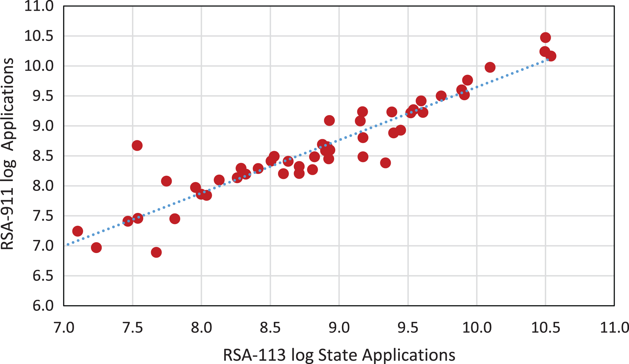
We can check how well the RSA-911 data fits 2015 applications disaggregated by state (but not by county) using the RSA-113 data. Figure 3 compares the log 2015 RSA-911 service recipients to the log 2015 RSA-113 service recipients. The OLS line best fitting the data is $log (RSA 911_{i}) = 0.809 + 0.884 log (RSA 113_{i}) + {error}_{i}$ with R² = 0.875. 16 A perfect fit would have the coefficient on the RSA-113 variable be 1 instead of 0.884 and have the constant be 0 instead of 0.809. However, the fit is excellent, and using logs implies only an error in the average state-specific fixed effect from Table 6.

Fig. 3

RSA-911 vs RSA-113 log Applications.

There are also limitations to these analyses based on using ACS data for population estimates. First, while ACS makes county level data available, the raw data is aggregated before release, making it impossible to evaluate individual level characteristics. ACS person-level data is available through the Public Use Microdata Sample (PUMS), but these data cannot be explored at geographies smaller than 100,000 people, known as Public Use Microdata Areas (PUMAs). As a result, data across counties (of varying type) are often combined, making it infeasible to parse out the geographic impact of residing in a noncore county.

Additionally, the ACS disability estimates are based on a set of 6-functional limitation questions that have been shown to underestimate specific disability groups, such as those with mental illness and learning and intellectual disabilities (Hall et al., 2012; Ipsen et al., 2018). The ACS functional limitation questions are also misaligned with definitions VR agencies use to classify applicants into disability type. This makes it difficult to explore more in-depth comparisons by disability type and questions about applicant case-mix variations across geographic setting (Ipsen & Swicegood, 2015).

Next, while the 6 functional limitation questions are used widely across national surveys, they often result in different estimates (Burkhauser, Houtenville, & Tennant, 2012). Using data from the Bureau of Labor Statistics (2019), we can compute disability rates by state. The range of rates is from 5.9% (in Hawaii) to 13.2% (in West Virginia) with a median of 8.2%. These are low compared to Kraus et al. (2018) who estimated a rate of 12.8% using the same data. Meanwhile, using the 2016 Behavioral Risk Factor Surveillance System data, Okoro et al. (2018) report that approximately 25% of the civilian population has a disability. 17 Undoubtedly, estimates vary substantially based on data samples, and conclusions could change if county level data were available and used from different data sets.

The final consideration we discuss is the use of only one year (FY 2015) of data. With one year of data, we can estimate state-specific fixed effects as was done and reported in Tables 4 and 6. If we want to explain the variation across states, we essentially have 50 degrees of freedom which is not much to estimate the effects of a reasonable set of potential explanatory variables. With multiple years of data, we can estimate year/state fixed effects and increase the degrees of freedom at least for those explanatory variables that change within states over the relevant time period.

Unfortunately, it was not until 2014 that RSA-911 data included geographic indicators including county and zip code information. Also, starting in the last quarter of FY 2017, RSA-911 data collection methods changed to a quarterly accounting of case progress in accordance with new Workforce Innovation and Opportunity Act regulations to increase program accountability. The small window of comparable data limits analyses.

5 Policy analysis and conclusions

The total effect of VR services on people with disabilities is A×B×C 18 where A is the probability of applying for VR services, B is a vector of probabilities of applying for different types of VR services, and C is a vector of the labor market outcome effects associated with using a particular set of services. Each of these effects depends on personal characteristics as well as state- and county-specific characteristics. Dean et al. (2015, 2017, 2018, 2019) and Schmidt et al. (2019) provide us with estimates of B and C. Dean et al. (2017) provide information about A but only for people with mental illness in Virginia in 2000, and Dean et al. (2019) provide information about A but only for transitioning youth in Virginia in 2000. Our results provide much more information about A.

What is missing from our analysis is the effect of individual characteristics on the probability of applying for VR services and, maybe more importantly, the change in that probability with the introduction of different changes in the environment and/or in relevant policy.

An important consideration is the effect of VR agency policy choices on the application probability. The data show wide variation in VR application rates across states based on the estimated state fixed effects in Tables 4 and 6. They also show significant variation in application rates across different county types. It is possible that VR policies and procedures are different in states with higher rural population rates, and are more effective in promoting VR services to eligible residents from rural counties. 19 Ipsen and Goe (2017) reported that programs serving a higher rural caseload utilized fee-for-service payment models and internal staff at higher rates than programs who served more urban caseloads and used performance-based funding and external vendors at higher rates. Fee for service delivery models and internal staff may support a more stable and ongoing VR presence in both rural and urban communities and result in more applications overall.

However, a test of the proposition that states with high rural population rates find ways to get rural people to apply is not supported by the data. Consider a linear regression where the dependent variable is the log ratio of the application rate in non-core counties over the application rate in metro counties and the explanatory variables are a constant and the log proportion of the population living in non-core counties. This regression has no statistical significance. This suggests that the proposition is incorrect.

While policies and procedures may be put in place to increase application probabilities, the costs associated with such efforts must also be considered. In part, application probabilities are shaped by available services and the costs associated with delivering those services. For example, VR programs use “order of selection” to ration VR services in financially strapped states. While order of selection does not prevent anyone from applying, it has a large effect on B, the probability of receiving VR services. This should have a significant effect on the probability of applying for services assuming there is some personal cost associated with the application process. Similarly, Schimmel Hyde et al. (2014) provide evidence on the effect of delaying service receipt on subsequent application for SSI benefits. 20

Overall, our results consistently show that people with disabilities living in rural counties are significantly less likely to take advantage of VR services. This runs counter to expectations based on indicators of eligibility and service need such as higher rural rates of disability and poverty. We do not know if this discrepancy is because of the personal costs associated with application and later service receipt, lack of information about available services, or negative perceptions of the likelihood that VR service receipt will result in employment at an acceptable wage. Unfortunately, however, a decision not to engage in VR services can have significant economic impacts. For instance, a large-scale longitudinal study of VR services showed that 89% of VR consumers whose cases were closed to competitive employment were still employed after one year, compared to 33.4% of individuals applying but choosing to forego VR services (Hayward & Schmidt, 2003).

While we have not been able to answer questions about the reasons people choose not to apply for services, we showed that application rates are systematically lower in rural counties. To improve parity across metro, micro, and noncore places, VR agencies might use national disability estimates to arrive at application benchmarks or targets across locations. At a minimum, this would provide information to VR programs about the effectiveness of various outreach efforts. This information might be combined with information about case-mix variations to develop targeted outreach efforts to underrepresented groups, including those from noncore and micro counties. It might also inform how VR service delivery models impact rural visibility and outreach. Future research might also focus on understanding the reasons fewer people with disabilities apply for VR services in rural communities.

Conflict of interest

None to report.

Footnotes

Appendix A: Weighting Issues

We weight the data presented in the last three columns of Table 1 by the number of people with disabilities (in the middle three columns of Table 1). We do this because each person represented makes an individual decision about whether to apply for VR services. Using county-specific data and the weights in ordinary least squares (OLS) or maximum likelihood estimation (MLE) is equivalent to performing the chosen econometric method using data on the individual people with disabilities.

One might worry that there is important unobserved heterogeneity, for example, at the county level which would imply less independent variation. However, our maximum likelihood estimates (Section 4.2) show that such heterogeneity is empirically unimportant in this particular example.

Table A.1 presents weighted moments of the critical variables (averaged over states and county types). The large number of observations comes from the fact that each person with a disability in each state and county type is a single observation. The weights used to translate state/county type aggregates into overall aggregates are the number of people in each state/county type cell seen in the middle three columns in Table 1.

The mean value of y, the proportion of disabled people who apply for vocational rehabilitation (VR) services, is 0.019, and the standard deviation is 0.009. Thus, in our sample, 1.9% of people with disabilities apply for VR services. The estimates show that 7.9% of our observations live in noncore counties, 10.9% live in micro counties, and 81.2% live in metro counties. The analogous rate for people without disabilities are 5.3%, 8.2%, and 86.5% respectively (ACS, S1810). This indicates that people with disabilities are more likely to live in rural counties than people without disabilities.

Table A.2 shows the weighted proportions of disabled people applying for VR services by county type (averaged across states). The corresponding mean proportions are 1.4% for noncore counties, 1.9% for micro counties, and 2.0% for metro counties.

Table A.1 shows the mean log(y) across states (averaged across county types). We transform the dependent variable using logs because it is easier to interpret the results and it fits the data better. 21 There is significant variation in the state averages with a standard deviation of 0.95. Vermont is somewhat of an outlier with a log proportion of –2.47 which is approximately 0.4 larger than the next two biggest states: Delaware and Utah. From Table 1, one can see that the application rates are high for each of the three county types in Vermont, but it is noncore counties in Vermont that are the outlier with an application rate of 11.4%. 22 It is not clear what critical factors make Vermont so different. At the other extreme, the states with the lowest mean log application rates are Puerto Rico (–9.2), Washington, DC (–6.6), and Georgia (–5.1).

Honeycutt et al. (2013) provide analogous estimates to those in Table 2 but for only transition-age youth with disabilities (and not disaggregated by county type). The application rates are much higher with the geometric mean of the state-specific ratios being 4.2; i.e., on average, transition-age youths with disabilities are 4.2 times as likely to apply for VR services than are all people with disabilities. This might have to do with VR outreach to transition students and emphasis on linking them with services before high school exit.

Appendix B: log Likelihood Contribution Construction

Using Equation (1), let (2) $y_{ijk} = 1 (y_{ijk}^{*} > 0)$ and $y_{ij} = \sum_{k = 1}^{K_{ij}} y_{ijk}$ . Equations (1) and (2) with δ= 0, along with data {i, j, y_ijk} _i,j,k imply estimation using the probit model (see, for example, Maddala, 1983; Wooldridge, 2002). However, instead, we observe only the choices made, aggregated over people within a county type and state, ${_{j = 1}^{J}}_{i = 1}^{n}$ .

The conditional likelihood contribution (given unobserved heterogeneity u_ij) for an observation (state and county type) is $\begin{matrix} L_{ij} (u_{ij}) = (\begin{matrix} K_{ij} \\ y_{ij} \end{matrix}) Φ (v_{ij} + δ u_{ij})^{y_{ij}} . \\ [1 - Φ (v_{ij} + δ u_{ij})]^{1 - y_{ij}} \end{matrix}$ where Φ(·) is the standard normal distribution function and $\begin{matrix} v_{ij} = β_{i} + 1 (j < J) α_{j} \end{matrix}$ is the non-random component of $y_{ijk}^{*}$ . The unconditional log likelihood contribution is

(3) $\begin{matrix} {logL}_{ij} = \log \int L_{ij} (u_{ij}) d Φ (u_{ij}) \\ = \log (\begin{matrix} K_{ij} \\ y_{ij} \end{matrix}) + \log \int Φ (v_{ij} + δ u_{ij})^{y_{ij}} . \\ [1 - Φ (v_{ij} + δ u_{ij})]^{1 - y_{ij}} d Φ (u_{ij}) . \end{matrix}$

The value of the vector of parameters (β, α, δ) that maximizes ∑_i,jlogL_ij is the maximum likelihood estimator (MLE) of the parameters. The MLEs are consistent and asymptotically efficient with known asymptotic covariance matrix (see, for example, Wooldridge, 2002).²³

Evaluation of the log likelihood function involves integration over the unobserved heterogeneity u_ij. Since the dimension of the unobserved heterogeneity in equation (3) is assumed to be 1, one could use numerical methods such as Gaussian quadrature to approximate the integral (for, example, Butler and Moffitt, 1982). 24

Alternatively, we use simulation methods to perform Maximum Simulated Likelihood (MSL) (see, for example, Dean et al., 2015). While it is well-understood that MSL is not consistent, work such as Börsch-Supan and Hajivassiliou (1993) provide strong evidence of good statistical behavior for MSL. In addition, we use antithetic acceleration (Geweke, 1988) to improve precision of our simulators.

The other issue of concern associated with estimation is that $(\begin{matrix} K_{ij} \\ y_{ij} \end{matrix})$ is very large, and the terms involving Φ(·), raised to a large power, are very small. This makes round-off error a significant issue. We can approximate $\log (\begin{matrix} K_{ij} \\ y_{ij} \end{matrix})$ well using Stirling’s formula to get $\begin{matrix} \log (\begin{matrix} K \\ y \end{matrix}) = - \log \sqrt{2 π} + (K + . 5) & logK - (y + . 5) logy - (K - y + . 5) log (K - y) . \end{matrix}$

Finally, we can simulate Equation (3) as $\begin{matrix} {logL}_{ij} = \log (\begin{matrix} K_{ij} \\ y_{ij} \end{matrix}) + K_{ij} M_{ij} + K_{ij} \\ \log \frac{1}{R} \sum_{r = 1}^{R} exp {(\frac{y_{ij}}{K_{ij}}) \log Φ (v_{ij} + δ u^{r}) \end{matrix}$ $\begin{matrix} + (\frac{K_{ij} - y_{ij}}{K_{ij}}) \log (v_{ij} + δ u^{r}) - M_{ij}) \end{matrix}$ where u^r is an iid draw from a standard normal distribution and $\begin{matrix} M_{ij} = \begin{matrix} max \\ r \end{matrix} [(\begin{matrix} y_{ij} \\ K_{ij} \end{matrix}) log Φ (v_{ij} + δ u^{r}) \\ + (\frac{K_{ij} - y_{ij}}{K_{ij}}) log (1 - Φ (v_{ij} + δ u^{r})] . \end{matrix}$

The presentation of the model in equations (1) and (2) informs the question of the degrees of freedom to assume in the linear models. If δ= 0, then each person with a disability is an independent observation, and aggregating to the state/county type level does not change that. In this case, the degrees of freedom for a specific state/county type is the total number of people with a disability in that state/county type K_ij. On the other hand, if δ is large, then the choices made by disabled people within a specific state/county type are highly correlated. In particular, as the parameters (β, α, δ) grow large (relative to the standard deviation of ɛ), the degrees of freedom for a specific state/county type converges to 1. Thus, the appropriate choice of degrees of freedom depends on the amount of unobserved heterogeneity δu_ij.

Appendix C: Bias Approximation

Dean et al. (2015) find that, for people with cognitive impairments, service receipt lasts for 3 quarters or less around 90% of the time (footnote 8). If we think of length of service receipt as an exponential random variable and assume the result from Dean et al. (2015) applies to all people receiving VR services, then this implies an exponential distribution parameter of 0.768. Further, if we assume that closures are uniformly distributed across the year, then the proportion of VR service recipients that closed in 2015 and started prior to 2015 is $\begin{matrix} \frac{1}{4} \int_{0}^{4} \int_{u}^{\infty} λ exp {- λ t} dtdu . \end{matrix}$ where λ = 0.768 is the exponential parameter. The integral is equal to 0.311. In words, given the assumptions made, 31.1% of the VR recipients in 2015 started their service receipt prior to 2015.

On the other hand, there may be people missing from the RSA-911 who applied for services in 2015 because they had not closed by the end of 2015. Making the same assumptions, the proportion of people in this group are $\begin{matrix} \frac{1}{4} \int_{0}^{4} exp {- λ (4 - u)} du = . 311 . \end{matrix}$

We use log() to denote the natural logarithm. Parameters should be interpreted as the proportional effect of the associated variable. See, for example, Azad (2020) for an intuitive explanation of natural logarithms.

States include Washington, DC and Puerto Rico.

Note that the standard deviation of ɛ is not identified in probit models.

Each of these three reported numbers is the exponent of the numbers reported in . For example, exp{-4.439)=0.0118.

The metro dummy is excluded, and its associated parameter is set to 0 to avoid the multicollinearity problem associated with including a full set of dummy variables, d_m with ∑_md_m = 1.

This also suggests that one could use random effects in a linear equation and save degrees of freedom. If we assume that each disabled person is an observation, there are more than enough degrees of freedom even with state-specific effects. If, instead, we assume that each state/county-type is an observation, then degrees of freedom are limited, and using random effects is possibly a better choice than fixed effects.

The relevant set of states are the 50 US states, Washington, DC, and Puerto Rico. Then Delaware, Washington, DC, New Jersey, Puerto Rico and Rhode Island are excluded because there is no variation in the county types in each state.

Standard errors are available from the corresponding author.

The results are somewhat similar to the mean log rates reported in Table A.3 in Appendix A with Vermont and Utah having large estimates (-0.879 and -1.242) and Georgia (-3.645), Louisiana (-3.337), Tennessee (-3.641), and Virginia (-3.124) having the smallest values.

As a general rule, $\frac{Δ \log y_{ij}}{Δ x_{ij}} = \frac{φ (x_{ij} α)}{y_{ij}} \frac{Δ y_{ijk}^{*}}{Δ x_{ij}}$ where φ (·) is the standard normal density function. The left-hand side of the equation corresponds to the estimates from Table 4, while $\frac{Δ y_{ijk}^{*}}{Δ x_{ij}}$ correspond to the estimates in Table 5. The first right-hand side ratio is of order $\frac{φ (Φ^{- 1} (0.03))}{0.03} = 2$ , thus explaining much of the variation between the estimates from Tables 3 and .

The VR application rate is approximately Φ(β_i + α_j) where Φ(·) is the standard normal distribution function, β_i is the relevant county type effect from Table 5, and α_j is the relevant county fixed effect from . We do not have to account for unobserved heterogeneity because of the very small estimate of δ.

One can think of the estimates in as approximately the parameter value that matches the predicted probabilities in each state to the sample probabilities in the state.

Information on which states were under an OOS regime, the size of the waiting list, and the number of applicants is available by VR agency at United States Department of Education (n.d.).

We exclude Washington, DC and Puerto Rico because they are outliers.

Stern et al. (2019) discuss the advantages of using VR data organized by application dates over VR data organized by closure dates.

The two outliers are Oregon (7.54, 8.67) and South Dakota (7.67, 6.89).

Johnson et al. (2017) report estimated prevalence for just mental illness of 10% from the National Health Interview Survey and 24% from the National Survey of Alcohol, Drug, and Mental Health Problems.

With a small abuse of notation, BxC really means the vector product of B’C.

Note that, to test this directly in our model, we would have to allow county type effects on application rates to vary with other covariates believed to affect them. Such covariates might include how states pay for services, the presence of VR offices in rural communities, and existing infrastructure, such as itinerant offices (required for counselors who serve a greater expanse). We did not do this, mostly because it would have been very difficult to gather the relevant information in a systematic way.

Order-of-selection effects and the Schimmel Hyde et al. (2014) effect are captured in our state fixed effect estimates.

Contact the corresponding author to get a copy of results in levels instead of logs.

One might wonder whether this is caused by sample error in the estimate of people with disabilities in noncore counties in Vermont. However, the disability rate in Vermont is a little above the median, and the standard error of the rate is 0.04%. Thus, that is not the source of the outlier.

In Dean et al. (2015, 2017, 2018, 2019) and Schmidt et al. (2019), the dimension of the unobserved heterogeneity is much larger than 1, ruling out Gaussian quadrature.

References

Aakvik,

, Heckman,

, & Vytlacil,

(2005). Estimating treatment effects for discrete outcomes when responses to treatment vary: An application to Norwegian vocational rehabilitation programs. Journal of Econometrics125, 15–51. doi:10.1016/j.jeconom.2004.04.002.

American Community Survey (ACS). 5 Year Summary File 2013-2017 [Table C18120 – Employment Status by Disability Status]. https://www.census.gov/programs-surveys/acs/data/summary-file.2015.html.

American Community Survey (ACS). 5 Year Summary File 2013-2017 [Table C18130 – Age by Disability Status by Poverty Status]. https://www.census.gov/programs-surveys/acs/data/summary-file.2015.html.

American Community Survey (ACS). 5 Year Summary File 2013-2017 [Table S1810 – Disability Characteristics]. https://www.census.gov/programs-surveys/acs/data/summary-file.2015.html.

Arkansas Research and Training Center on Vocational Rehabilitation (1992). President’s Committee on Employment of People with Disabilities. Employment Priorities for the 90s for People with Disabilities.

Azad,

(2020). Demystifying the natural logarithm (ln). Better Explained. https://betterexplained.com/articles/demystifying-the-natural-logarithm-ln/.

Bearse,

, Gurmu,

, Rapaport,

, & Stern,

(2004). Estimating disabled people’s Demand for specialized transportation. Transportation Research38(9), 809–831. https://doi.org/10.1016/j.trb.2003.10.004

Börsch-Supan,

, & Hajivassiliou,

(1993). Smooth unbiased multivariate probability simulators for maximum likelihood estimation of limited dependent variable models. Journal of Econometrics58(3), 347–368. doi:10.1016/0304-4076(93)90049-B.

Bureau of Labor Statistics. (2019). Local Area Unemployment Statistics. United States Department of Labor. https://www.bls.gov/lau/ptable14full2018.htm.

10.

Burkhauser,

, Houtenville,

, & Tennant,

(2012). Capturing the elusive working-age population with disabilities: Reconciling conflicting social success estimates from the Current Population Survey and American Community Survey. Journal of Disability Policy Studies24(4), 195–205. doi:10.1177/1044207312446226.

11.

Butler,

J. S.

, & Moffitt,

(1982). A computationally efficient quadrature procedure for the one-factor multinomial probit model. Econometrica50(3), 761–764. doi:10.2307/1912613.

12.

Clapp,

, Stern,

, & Yu,

(2019). Interactions of public paratransit and vocational rehabilitation [Unpublished manuscript]. https://drive.google.com/file/d/1D9P-VoIoqzej6yg2KY8pouTjofGKjl0x/view

13.

Dean,

, Pepper,

, Schmidt,

, & Stern,

(2015). The effects of vocational rehabilitation for people with cognitive impairments. International Economic Review56(2), 399–426. doi:10.1111/iere.12109.

14.

Dean,

, Pepper,

, Schmidt,

, & Stern,

(2017). The effects of vocational rehabilitation services for people with mental illness. Journal of Human Resources52(3), 826–858. doi:10.3368/jhr.52.3.0114-6111R1.

15.

Dean,

, Pepper,

, Schmidt,

, & Stern,

(2018). The effects of vocational rehabilitation for people with physical impairments. Journal of Human Capital12(1), 1–37. doi:10.1086/696098.

16.

Dean,

, Pepper,

, Schmidt,

, & Stern,

(2019). The effects of youth transition programs on labor market outcomes. Economics of Education Review68, 68–88. doi:10.1016/j.econedurev.2018.11.006.

17.

Erickson,

W. A.

, VanLooy,

, von Schrader,

, & Bruyère,

(2018). (2018). Disability, income, and rural poverty. In D. Harley, N. Ysasi, M. Bishop, & A. Fleming (Eds.), Disability and vocational rehabilitation in rural settings (pp. 17-41). Springer.

18.

Geweke,

(1988). Antithetic acceleration of Monte Carlo integration in Bayesian inference. Journal of Econometrics38(1/2), 73–89. doi:10.1016/0304-4076(88)90027-9.

19.

Hall,

, Kurth,

, & Fall,

(2012). Discrepancy among Behavioral Risk Factor Surveillance System, Social Security, and Functional Disability Measurement. Disability and Health Journal2, 60–63. doi:10.1016/j.dhjo.2011.08.004.

20.

Hamilton,

, Jungheim,

, McManus,

, & Pantano,

(2018). Healthcare access, costs, and treatment dynamics: Evidence fromfertilization. American Economic Review108, 3725–3777. doi:10.1257/aer.20161014.

21.

Hayward,

, & Schmidt-Davis,

(2003). Longitudinal Study of the Vocational Rehabilitation Services Program: Final Report 2: VR services and outcomes. Research Triangle Institute. https://www2.ed.gov/rschstat/eval/rehab/vr-final-report-2.pdf.

22.

Heckman,

(1979). Sample selection bias as a specification error. Econometrica47(1), 153–161. doi:10.2307/1912352.

23.

Heckman,

, Lalonde,

, & Smith,

(1999). The economics and econometrics of active labormarket programs. In O. Ashenfelter & D. Card (Eds.), Handbook of labor economics (Vol 3A; pp. 1865-2097). North Holland.

24.

Henderson,

(2011). Proposed ACA data collection standards. Disability Rights Education and Defense Fund. https://dredf.org/2011/08/01/proposed-aca-data-collection-standards/.

25.

Honeycutt,

, Thompkins,

, Bardos,

, & Stern,

(2013). State differences in the vocational rehabilitation experiences of transition-age youth with disabilities. Journal of Vocational Rehabilitation42, 17–30. doi:10.3233/JVR-140721.

26.

Imbens,

, & Wooldridge,

(2009). Recent developments in the econometrics of program evaluation.”. Journal of Economic Literature47(1), 5–86. https://www.aeaweb.org/articles?id=10.1257/jel.47.1.5

27.

Ipsen,

(2012). Transportation: A barrier to successful employment outcomes among rural VR clients. Research Report. The University of Montana Rural Institute. https://scholarworks.umt.edu/ruralinst_employment/15/

28.

Ipsen,

, Chambless,

, Kurth,

, McCormick,

, Goe,

, & Hall,

(2018). Underrepresentation of youth with mental and development disabilities using American Community Survey (ACS) questions. Journal of Disability and Health11, 447–450. doi:10.1016/j.dhjo.2017.11.005.

29.

Ipsen,

, & Goe,

(2017). Effective rural VR job development. A State of the Science Symposium conducted online at the University of Montana Rural Institute, Missoula, MT. http://rtc.ruralinstitute.umt.edu/knowledge-translation/state-of-the-science/rural-vr-sos/.

30.

Ipsen,

, Goe,

, & Bliss,

(2019). Vocational rehabilitation (VR) funding of job development and placement services: Implications for rural reach. Journal of Vocational Rehabilitation51(3), 313–324. doi:10.3233/JVR-191048.

31.

Ipsen,

, Rigles,

, Arnold,

, & Seekins,

(2012). The use of telecommunications to deliver services to rural and urban vocational rehabilitation clients. Rehabilitation Counseling Bulletin55(3), 144–155. doi:10.1177/0034355211432892.

32.

Ipsen,

, & Swicegood,

(2015). Rural and urban differences in vocational rehabilitation case mix, delivery practices, and employment outcomes. Rehabilitation Research Policy and Education29(4), 349–370. https://connect.springerpub.com/content/sgrrrpe/29/4/349

33.

Ipsen,

, & Swicegood,

(2017). Rural and urban vocational rehabilitation self-employment outcomes. Journal of Vocational Rehabilitation, 46(1), 97–105. doi:10.3233/JVR-160846.

34.

Johnson,

, LaForest,

, Lissenden,

, & Stern,

(2017). Variation in mental illness and provision of public services in Virginia. Health Services and Outcomes Research Methodology17(1), 1–30. https://link-springer-com-443.web.bisu.edu.cn/article/10.1007/s10742-016-0167-3

35.

Jolly,

, Priestley, , & Matthews,

(2006). Secondary analysis of existing data on disabled people’s use and experiences of public transport in Great Britain. Disability Rights Commission. https://disability-studies.leeds.ac.uk/wp-content/uploads/sites/40/2011/10/DRC-transport-campaign-research-report-October-2006.pdf

36.

Kaya,

, Chan,

, Rumrill,

, Hartman,

, Wehman,

, Iwanaga,

, Pai,

C.-H.

, & Avellone,

(2016). Vocational rehabilitation services and competitive employment for transition-age youth with autism spectrum disorders. Journal of Vocational Rehabilitation45(1), 73–83. doi:10.3233/JVR-160812.

37.

Kraus,

, Lauer,

, Coleman,

, & Houtenville,

(2018). 2017 Disability Statistics Annual Report. University of New Hampshire. https://files.eric.ed.gov/fulltext/ED583258.pdf

38.

Langi,

, & Balcazar,

(2017). Risk factors for failure to enter vocational rehabilitation services among individuals with disabilities. Disability and Rehabilitation39(26), 2640–2647. https://www-tandfonline-com-s.web.bisu.edu.cn/doi/full/10.1080/09638288.2016.1236410

39.

Maddala,

(1983). Limited-dependent and qualitative variables in econometrics. Cambridge University Press.

40.

Mattson,

(2015). Rural transit fact book 2015. Small Urban and Rural Transit Center, Upper Great Plains Transportation Institute, North Dakota State University. https://www.ugpti.org/surcom/resources/transitfactbook/downloads/2017-rural-transit-fact-book.pdf

41.

McDaniels,

, Harley,

, & Beach,

(2018). Transportation, accessibility, and accommodation in rural communities. In D. Harley, N. Ysasi, M. Bishop, & A. Fleming (Eds.), Disability and vocational rehabilitation in rural settings (pp. 43-57). Springer.

42.

National Council on Disability. (2005). The current state of transportation for people with disabilities in the United States. https://ncd.gov/publications/2005/current-state-transportation-people-disabilities-united-states.

43.

Okoro,

, Hollis,

, Cyrus,

, & Griffin-Blake,

(2018). Prevalence of disabilities and health care access by disability status and type among adults — United States, 2016. Morbidity and Mortality Weekly Report67(32), 882–887. https://www.cdc.gov/mmwr/volumes/67/wr/mm6732a3.htm

44.

Rigles,

, Ipsen,

, Arnold,

, & Seekins,

(2011). Experiences of rural vocational rehabilitation clients who leave the system prematurely: A qualitative exploration. Rehabilitation Counseling Bulletin, 54(3)164–174. doi:10.1177/0034355210396948.

45.

Sabella,

, Bezyak,

, & Gattis,

(2016). Barriers to public transportation: The impact on employment of individuals with disabilities [Unpublished manuscript].

46.

Schimmel Hyde,

, Honeycutt,

, & Stapleton,

(2014). The relationship between timely delivery of vocational rehabilitation services and subsequent federal disability benefit application and receipt. IZA Journal of Labor Policy3, 15. doi:10.1186/2193-9004-3-15.

47.

Schmidt,

, Clapp,

, Pepper,

, & Stern,

(2019). What do ROI estimation models say about ROI in Virginia and Maryland?. Journal of Rehabilitation Administration40(1), 57–72.

48.

Stern,

(1993). A disaggregate discrete choice model of transportation demand by elderly and disabled people in rural Virginia. Transportation Research Part A: Policy and Practice27(4), 315–327. doi:10.1016/0965-8564(93)90004-5.

49.

Stern,

, Clapp,

, Pepper,

, & Schmidt,

(2019). Data issues in developing valid ROI/ROR estimates. Journal of Rehabilitation Administration40(1), 35–46.

50.

United StatesDepartment ofDisability Services. (n.d.).Vocational Rehabilitation Services. https://dds.dc.gov/service/vocational-rehabilitation-services.

51.

United States Department of Education (n.d.). https://rsa.ed.gov/view.cfm?rsaform=RSA-113.

52.

West,

, Hock,

, Wittig,

, & Dowdy,

(1998). Getting to work: Training and support for transportation needs. Journal of Vocational Rehabilitation,159–167. doi:10.3233/JVR-1998-10210.

53.

Wooldridge, , & Jeffrey, (2002). Econometric analysis of cross section and panel data. MIT Press.

54.

Ysasi,

, Lebogang,

, Sprong,

, & Kim,

B. J.

(2018). Marketing vocational rehabilitation services in rural communities. In D. Harley, N. Ysasi, M. Bishop, & A. Fleming (Eds.), Disability and vocational rehabilitation in rural settings (pp. 545-552). Springer.

The effect of ruralness on vocational rehabilitation applications

Abstract

BACKGROUND:

OBJECTIVE:

METHODS:

RESULTS:

CONCLUSIONS:

Keywords

1 Introduction

1.1 Variation in VR application rates

1.2 Data

3.1 OLS estimates

Table 2 OLS estimates in levels without state specific effects Variable Estimate Std Err t-Statistic Noncore –4.9439** 0.001 –7,394.600 Micro –4.186** 0.001 –8,193.000 Metro –3.987** 0.000 –21,276.300

Table 5 MSL Estimates Other than State-Specific Fixed Effects Estimate Std Err Noncore –0.176** 0.0005 Micro –0.066** 0.0003 Delta 0.0004 0.0089

Conflict of interest

Footnotes

Appendix A: Weighting Issues

Appendix B: log Likelihood Contribution Construction

Appendix C: Bias Approximation

References

Table 2
OLS estimates in levels without state specific effects

Variable Estimate Std Err t-Statistic

Noncore –4.9439^ 0.001 –7,394.600

Micro –4.186^ 0.001 –8,193.000

Metro –3.987^** 0.000 –21,276.300

Table 5
MSL Estimates Other than State-Specific Fixed Effects

Estimate Std Err

Noncore –0.176^ 0.0005

Micro –0.066^ 0.0003

Delta 0.0004 0.0089