Autonomic communication system based on cognitive techniques

Abstract

In modern communication systems, it is necessary to develop new approaches to optimize them. To achieve this objective, new paradigms are necessary. The present work proposes an autonomic communication system, which uses a system of decision-making based on a Bayesian network, and a knowledge base based on an ontology, to take decisions of reconfiguration in the system. The main goal of the autonomic communication system is to adapt the communications platform to the characteristics of the context, in order to improve its performance. The ontology provides the knowledge about the performance factors and their relationships in the communication networks, to configure the structure of the Bayesian network. The Bayesian network is the stochastic reasoning mechanism used by the decision-making system. We present several tests on the NS2 simulator. In the tests carried out, we observe an improvement between 85% and 96% in the system performance, for scenarios where our approach of autonomic decision reconfigures the communication system.

Keywords

Autonomic communication system autonomous systems Bayesian network ontology

1. Introduction

1.1 Research background

Currently, due to the great number of devices of interconnection, to the technologies of interconnection, and to the development of new communication platforms, we have a diversity of available mass media. On the other hand, the multimedia applications are more common every day, and the real time communications need of major bandwidths, minor latencies, minor variation in the time of arrival of packages (jitter), major reliability, and in general, of sensitive environments to variations in the flow (throughput). In this way, it is necessary to optimize the use of the resources of the communication networks. One answer to these necessities, it is to develop self-configurable communication systems; that is, it is required the development of autonomous communication systems that improve their performance.

In that sense, this work proposes an autonomic communication system that optimizes its performance, as a function of what it knows about the context (data transmission problems, etc.) and of the applications running on it (multimedia or not, with or without quality of service, etc.). The autonomic communication system requires of a decision-making system to guide the reconfiguration process, in order to adapt it to the new operational conditions. In our case, the system of autonomous decision requires of an ontology that describes the communication system, the autonomous tasks to carry out the reconfiguration process, among other things. Moreover, with our ontology is developed a decision Bayesian model, which is updated through a learning process, in order to adapt its behavior based on the changes in the operational context. So, we propose to develop an autonomous decision system based on an ontology, from which is conceived a Bayesian network as an inference mechanism for decision making. The main idea of using Bayesian networks is because they allow the management of uncertainty, typical in the systems of communication. The principle of the autonomic communication system proposed in this work is to make intelligent decisions based on the ontologies and Bayesian networks.

1.2 Literature review

The autonomous communication systems have been inspired by the autonomic computing, with the goal of allowing the self-configuration, self-management and self-regulation of the communication infrastructures. Some works in autonomic communication systems are [10, 17, 23, 3, 1, 26]. The topics most developed in autonomic communication are: the development and implementation of an autonomic communication kit (ACT) for a communication system that meets its requirements of quality of service (QoS) [26]. This work uses the Markov chains for taking decisions about whether the system must be or not reconfigured, and proposes a theoretical model of reinforcement learning to optimize the communication systems. Another work is proposed in [20], which used cognitive networks and influence diagrams to make decisions about how to improve the communication. Finally, a work linked to the problem of autonomic reconfiguration is proposed in the DAISY project (Diagnosis for Adaptive Strategies in collaborative systems). In particular, this project proposes an architecture of an autonomous system of communication, which is based on the identification of the current situation in the communication system; they propose an approach to invoke the process of self-adaptation, which ensures that the system is able to continue functioning properly [2].

In decision-making of self-adaptive systems (SASs), [6] proposes a methodological specification that uses dynamic networks of decision based on Bayesian networks, enriched with a short-term memory, to improve the performance in decision-making processes with uncertainty. In intelligent decision systems based on ontologies, the doctoral thesis [30], at INSA-Toulouse, uses an ontology based on the ODA (Ontology Driven Architecture) paradigm, for the autonomous management of the quality of service in communications networks. It defines a framework based on ontologies, to develop an autonomous system of communications. This ontology allows describing the QoS requirements, so as to enable an autonomic process in the communication system that provides the required QoS.

Finally, Bayesian networks can represent uncertainty in the relationship of dependency between variables that describe a process of decision making (in our case, linked to communication systems) [7, 25, 5]. The learning in the Bayesian networks can be divided into two types [24]: parametric and structural. In particular, several works propose methodologies for the construction of Bayesian networks by means of ontologies. For example, in [21] proposes a framework called BayesOWL, which specifies a formal method for the creation of Bayesian networks from ontologies that allows the handling of uncertainty over the domain for which it was designed the ontology.

1.3 Paper positioning

The main contribution of this work is the definition of an autonomic communication system based on an ontology used to build a Bayesian network that is defined for the decision-making process of reconfiguration. With respect to previous works, it is used an ontology based on the mix of several ontologies of references of communication systems, which provides a knowledge base for the system of decision-making. With this ontology is built a Bayesian network, which makes that the system be able to deal with the uncertainty typical of the communication systems. The Bayesian network is used to choose the action of reconfiguration that maximize the performance of the communication network. In addition, the autonomous system can predict with effectiveness the trend of performance of the communication network, in order to prevent its degradation. In addition, the system is able to learn, so as to update the parameters of the Bayesian network, to reconfigure the communicational platform according to the current information. Finally, the system can make decisions with partial or total information about the communication system.

This paper is organized as follows: Section 2 presents

the theoretical framework, specifically, the communication systems from the point of view of the autonomous systems, and the Bayesian networks for decision-making processes, and how they are constr- ucted from ontological frameworks. Section 3 presents the architecture of our autonomous system based on Bayesian Networks, as well as the process of transformation of the ontology to the Bayesian network to be used in the autonomous system. Section 4 details the experiments, and the results are analyzed. Finally, the conclusions and recommendations are presented.

Figure 1.

Architecture for self-adaptation [2].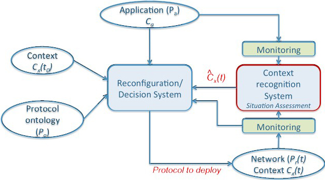

2. Theoretical frameworks

2.1 Autonomic communication systems

The autonomic communication is an extension of the concept of autonomic computing, which is applied to the communication networks. In general, an autonomic communication system must monitor, analyze, take decisions and act, in the communication platform. An autonomic communication must self-configure, self-optimize, self-protect and self-heal, with minimal human intervention, to adapt it to the changes to its context.

The paradigm of Autonomic Computing (AC) is inspired by the autonomous nervous system of the human being. Its fundamental objective is that the computer systems can be self-managing. An autonomous system takes decisions by its account, using high-level policies, to review and to constantly optimize its situation, and adapt to the changing conditions of its environment [27, 3, 17]. The architecture of an autonomic system has been described in [16]. The components are:

•
Managed Resource: Can be any type of resources (hardware or software) that can be managed. The managed resources are controlled through its sensors and actuators.
•
Touch Points: Binds to the sensors and/or actuators required for the management of resources.
•
Autonomic Local Manager: Implements the intelligent control loops that automate the tasks of self-management. The components of the control loop, which share a common knowledge base, are:

–
Monitoring Component: It provides mechanisms for the collection of the information about the resources to be handled.
–
Analysis Component: It provides mechanisms to correlate and model complex situations, to analyze that may be occurring in the system. These mechanisms allow understanding the current situation, inferring future situations, among other things.
–
Planning Component: Provides mechanisms for the constructing and planning of the actions necessary to meet the goals of the autonomous system.
–
Execution Component: Defines mechanisms that execute the actions defined in the planning component, to reach the goals of the system.

These four components, with the component of knowledge representation, define the control loop.

•
Orchestrator of the Autonomic Managers: Due to an autonomous system can count with several local managers, which need to work together to ensure the correct operation of the system, this level provides the communication channel for the coordination between them.
•
Manual Manager: Allows to humans configure the autonomic managers to perform their task of self-management, providing for this a man-machine interface.
•
Sources of Knowledge: Provides access to the knowledge required for the autonomic system.

An example of an autonomic communication system is DAISY [2], which is shown in Fig. 1. In this architecture, the reconfiguration process takes into consideration different entries:

•
$\bm{P_{0}}$ , properties of the different protocols specified in an ontology.
•
The initial context $\bm{C_{x}(t_{0})}$ .
•
The properties required by the application $\bm{P_{a}}$ , and in particular, the context required $\bm{C_{a}}$ .
•
The current state of the context $\bm{C_{x}(t)}$ , and the suggested modifications to the context $\bm{\hat{C}_{x}(t)}$ .

DAISY architecture is based on a system of recognition of context, which monitors and evaluates the context of the communication system, to propose changes on the same.

The autonomic communication is a concept than, in addition to the concepts derived from the autonomic computing, also we can add some other principles, such as: advanced handling of the communication platform in aspects such as the virtualization of the network, the specialized management of certain applications on the network (telephony, video conference, etc.), support systems to communications (disaster recovery, etc.), the incorporation of the management of applications as a service (SaaS), among others.
2.2 Bayesian networks

Bayesian networks (RB), also known as networks of beliefs, belong to the family of probabilistic graph models. These structures of directed graphs are used to represent uncertain knowledge as a multivariate probability model, which describes a set of random variables and their causal influences [7]. In the RB, each node represents a random variable, and the arcs represent probabilistic dependencies between the variables (the absence of the arcs indicates conditional independence). Uncertainty displayed in RB can be modified based on the events on the real system monitored.

A RB represents knowledge through causal relationships (structure of the graph) characterized by conditional probability tables between nodes. Thus, the knowledge network is composed of the following elements [18]:

•
A set of nodes that represent each variable in the model.
•
A set of arcs between the nodes that have a causal relationship.
•
A table of conditional probabilities associated with each node, indicating the probability of its states for each combination of the states of its parents.

The inference process in the RB is based on the Bayes Theorem [18]. In the RB, the probabilistic inference consists in, given certain known variables (evidence), calculate the probability of the other variables (unknown). The Bayes theorem expresses the conditional probability of a random event $h_{i}$ , given $x$ , in terms of the distribution of the conditional probability of the event $x$ , given $h_{i}$ , and the marginal probability distribution of only $h_{i}$ (see Eq. (1)).

$\displaystyle P\left(h_{i}|x\right)=\frac{P\left(x|h_{i}\right)P(h_{i})}{P(x)}$ (1)

where $P(h_{i})$ is the probability of $h_{i}$ , $P(x|h_{i})$ is the probability of $x$ given the hypothesis $h_{i}$ , $P(h_{i}|x)$ is the probability of $h_{i}$ given the evidence $x$ .

In general, this model can be extended considering the constraints $T$ , in such a way to determine the hypothesis $h$ about the problem that is being explored, given the observed data $x$ , the restrictions $T$ , and the other assumptions about the problem [25] (see Eq. (2)).

$\displaystyle P\left(h|{x,T}\right)=\frac{P\left(x|{h,T}\right)P\left(h|T% \right)}{\sum\nolimits_{h^{\prime}\in H_{T}}{P\left(x|{h^{\prime},T}\right)P% \left(h^{\prime}|T\right)}}$ (2)

where, the domain $T$ generates a space of hypothesis candidates, called $H_{T}$ . The probability $(x|h,T)$ measures how well each scenario predicts the data, and the probability $(h|T)$ expresses the truth of the hypothesis given the prior knowledge $T$ . The probability $P(h|x,T)$ is proportional to the product of these two terms, that represent the degree of belief in this hypothesis, given the previous restrictions $T$ and what has been observed in the $x$ data, divided by the sum of the degree of belief en each hypothesis [25].

The learning in the RB consists in the development of a model of the structure, and the definition of the parameters of the network, from the data in the system to monitor [24]. In this way, the learning can be in two ways [24].
2.2.1 Parametric learning

It is based on the fact that, given the structure, must be obtained the associated probabilities. There are many methods in the literature for the parametric learning, in this work were used [7, 19].

Learning by method of maximizing the expectation

The method of learning of the method of EM (EM, expectation maximization) is very used in the case of hidden nodes. The hidden nodes are defined as the nodes where the values that a variable can have are not known. The algorithm of this method is [24, 13]:

1.
Start the unknown parameters (conditional probabilities) with random values (or estimated by experts): $\theta^{[t]}_{2}=\{\theta_{1}^{[t]}\theta_{2}^{[t]},\ldots,\theta_{c}^{[t]}\}$ .
2.
Use the known data, with the current parameters $\theta_{c}^{[t]}$ , to estimate the values of the unknown variables (this Step is called Step E, by estimation), where $t$ is the iteration index, ${\cal F}$ is the auxiliary function defined in Eq. (3), $x=(x_{1},x_{2},\ldots,x_{n})$ are the observed data, $z=(z_{1},z_{2},\ldots,z_{n})$ are the unknown variables, and $q$ is a distribution on the variables $z$ .

$\displaystyle P\sum\limits_{z}{q(z|x)\log{\frac{p(x,z|\theta)}{q(z|x)}}}% \triangleq\mathcal{F}(q\theta)$ (3) $\displaystyle q_{c}^{\left[t+1\right]}\leftarrow\underset{q}{\rm argmax}\ {% \mathcal{F}(q,\theta_{c}^{\left[t\right]})}$ (4)
3.
Use the values estimated in the previous Step $q_{\left[t+1\right]}$ to complete the data table (this Step is called Step M, by maximization).

$\displaystyle\theta_{c}^{\left[t+1\right]}\leftarrow{\underset{\theta}{\rm argmax% }\ \mathcal{F}(q_{c}^{\left[t+1\right]},\theta_{c})}$ (5)
4.
Repeat Steps 2 and 4 until there are no significant changes in the odds.

2.2.2 Counting-learning

Learning by counting is the method simplest and fastest, when there are not many missing data or many uncertain data. The counting method can be used to learn or reinforce the conditional probability tables (CPT).

In the case of learning, this method part of a network that is in a state of total ignorance, in which all the probabilities are uniform. The mechanism allows to learn the probabilities. The other case in which this method is used is to reinforce the learning. In both cases, the next procedure is followed [19]:

For the nodes of the network in which there is a finding (for example, there is a finding for a given node ( $I_{x}$ ) and its parents ( $P_{x-z}$ ), where $z$ is the number of parents of the node), they are modified, so that their experiences and individual probabilities are modified ( $I_{x}$ ) (the conditional probability from its parents to the node ( $I_{x}$ ) is updated). The new experience ( $\textit{experience}_{I_{x}}^{n}$ ) is obtained by taking the previous value of $\textit{experience}_{I_{x}}^{n-1}$ , and add the new belief, to represent the new experience, as is shown in the Eq. (6) [19].

$\displaystyle\textit{experience}_{I_{x}}^{n}=\textit{experience}_{I_{x}}^{n-1}% +\textit{belief}$ (6)

The belief generally takes the value of 1, but the same can have a higher value, as for example 2, if there are two identical cases at once. Additionally, it can take the value of $-$ 1 to forget the value [19]. Now, in the vector of probability, it changes from $\textit{probability}_{I_{x}}^{n-1}$ to $\textit{probability}_{I_{x}}^{n}$ , as is described in the Eq. (2.2.2) [19]:

$\displaystyle\textit{probability}_{I_{x}}^{n}=$ $\displaystyle\frac{(\textit{probability}_{I_{x}}^{n-1}*\textit{experience}_{I_% {x}}^{n-1}+\textit{belief })}{\textit{experience}_{I_{x}}^{n}}$ (7)

The probabilities of the brothers of $I_{x}$ in this vector (the siblings of a node are the nodes that have the same parent as it), change according to the Eq. (8):

$\displaystyle\textit{probability}_{i}^{n}=\frac{\textit{probability}_{i}^{n-1}% *\textit{experience}_{I_{x}}^{n-1}}{\textit{experience}_{I_{x}}^{n}}$ (8)

In this way, the new vector is normalized according to the factor of $\textit{experience}^{n}$ .

2.2.3 Structural learning

Structural learning consists mainly of getting the structure or topology of the network, that is, finding the dependency relationships between the different variables. These relationships can be found mainly in two ways; the first is to obtain the structure from an expert, and the second is to use data mining to obtain the structure. The second case, according to the type of structure, can use the methods [24].

•
Trees Learning.
•
Polytree Learning.

In both cases the problem is about optimization, to obtain the tree structure that is closest to the’real’ distribution. For the majority of the cases is used the algorithm of Chow-Liu [7]. The Chow-Liu algorithm assumes that each variable has at most one root (father node), and is based on approximate a probability distribution from a probability product of second order. In the Chow-Liu algorithm, the joint probability of n variables is expressed by the equation:

$\displaystyle P\left(X_{1},X_{2},\ldots,X_{n}\right)=\prod\limits_{i=1}^{n}P(X% _{i}|X_{j(i)})$ (9)

where $X_{j(i)}$ is the father of $X_{i}$ .

To obtain the structure of the network is optimized a measure of the difference of the information (DI) between the actual distribution $P$ and the approximate $P$ , by means of the Eq. (10). The objective is to minimize DI [24].

$\displaystyle\textit{DI}\left(P,P^{}\right)=\sum\limits_{X}{P(x)\textit{Log}% \frac{P(x)}{P^{*}(x)}}$ (10)

We can define this difference in function of the information ( $I$ ) between the variables, according to the Eq. (11):

$\displaystyle I(X_{i},X_{j})=\sum\limits_{X_{i},X_{j}}{P(X_{i},X_{j})\textit{% Log}\frac{P(X_{i},X_{j})}{{P(X}_{i})P(X_{j})}}$ (11)

Finally, the optimal tree is found by the algorithm [24, 29]:

1.
Create an empty $\beta$ graph, with $\eta$ as the set of vertices.
2.
Calculate the mutual information between all pairs of variables (in general). For this is used the Eq. (11).
3.
Sort the mutual information from highest to lowest.
4.
Add the arc with the largest value of mutual information to graph $\beta$ .
5.
Add the following arc while it does not form a cycle, otherwise discard.
6.
Repeat Steps 3 to 5 until cover all variables $\eta$ are considered.

This kind of learning is not required for this work.
2.3 Decision making in Bayesian networks and diagram of influence

Decision-making in Bayesian networks is not only based on the probability of an event, but also the potential benefits (utilities) and the costs of the same, in order to determine how it affects the possible decision. The main idea is to be able to find a plan of action to maximize the benefits and minimize the costs. In this way, Bayesian networks have been extended to handle the theory of decisions.

To do this, the Bayesian network defines influence diagrams, which is an extended version of it. The influence diagrams have three types of nodes, the first corresponds to nodes of the RB original (uncertain), the second are nodes corresponding to the actions to be taken (decision), and finally, the last nodes corresponding to the utility function (see Fig. 2). A node of function of utility is represented by a diamond, and an action node as a box.

The influence diagrams [31] are used to make decisions that will maximize the benefits of the actions to be implemented, based on the expected utility (MUE). In that sense, solving a decision problem is equivalent to determine the maximum expected utility using the chosen strategy. The utility of the action $a_{i}$ ( $a_{i}\in A$ , where $A$ are the alternatives $a_{1},a_{2},\ldots,a_{m}$ ) under the hypothesis $h_{j}$ is $\mu$ ( $a_{i}$ , $h_{j}$ ), where $\mu$ ( ) is the utility function. In this way, the utility to perform the action $a_{i}$ is given by the Eq. (12), where $P$ ( ) represents the conditional probability of $H$ (set of hypotheses $h_{1},h_{2},\ldots,h_{n}$ ) given $\varepsilon$ , and $\varepsilon$ is a set of observations in the form of evidence in a given time [18]:

$\displaystyle\mathrm{UE}(a_{i})=\sum\limits_{j}{\mu\left(a_{i},h_{j}\right)}P(% h_{j}|\varepsilon)$ (12)

The MUE is obtained as the maximum result of UE( $A$ ):

$\displaystyle a^{*}=\mathrm{arg}∼{}\underset{a_{i}\in A}{\max}∼{}{\mathrm{EU}(% a_{i})}$ (13)

Thus, a diagram of influence can be considered as a Bayesian network augmented with decision variables, the utility functions that specify preferences in the decision-making, and an order of precedence.

Figure 2.

Example of diagram of influence.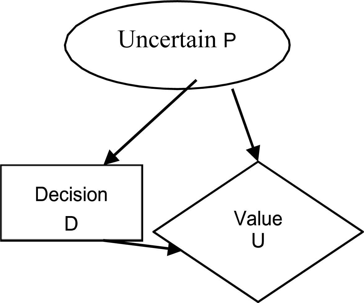

Formally, a diagram of influence is a directed acyclic graph (DAG) that contains N nodes representing the variables of the problem of decision $V=X\cup D\cup U$ . Each variable has its own domain dom( $v$ ), and a set of parents $v_{i}$ implicated by $\pi_{vi}$ . The three types of variables in a diagram of influence are [9]:

•

Uncertain Nodes, $x_{i}\in X$ , represent the random variables of the diagram. They have associated CPTs, representing the distribution $P$ ( $x_{i}$ , $\pi_{xi}$ ).

•

Decision Nodes, $d_{i}\in D$ , represent the decisions to be taken, the decision rules $\delta_{i}$ represent the mapping of the parent nodes to a decision, $\delta_{i}(\pi_{di})\in$ dom $(d_{i})$ .

•

Utility Nodes, $u_{i}\in U$ , represent features that result from the mapping of the parent nodes, with a value of utility val ${}_{u}(\pi_{vi})\in$ dom $(u_{i})$ . None of the nodes of utility have offspring.

The CPT represents the quantitative information about the probabilistic network, the same is represented as a real number in the range [0.1]. The CPT is a simple table, which has a numeric value for each possible combination of a parent node with its child nodes, which represents the conditional probability of occurrence of the son given that occurs the father (Bayes theorem). All the probabilities that come out of a parent node must sum 1 [19].

In a diagram of influence are seeking, in general, take the optimum decision, which is the one that maximizes the value of utility. When there is no quantification, simply is limited to choose the possible actions.

3. Process of transformation of an ontology to a Bayesian network

There are multiple jobs that address the transformation of an ontology in a Bayesian network [14, 15, 21]. In particular, in this work we use the framework BayesOWL. The framework BayesOWL [22] provides a set of rules and procedures for the direct transformation of an ontology described in OWL in a Bayesian network. BayesOWL allows:

•
Represent information of OWL as probabilities.
•
Translate OWL ontologies to RB.

–
Rules to build the structure of the RB from triplets OWL.
–
Help for the addition of special nodes for the logical relationships.
–
Construction of tables CPT.

3.1 Structural translation

For the structural translation of an ontology described in OWL in a Bayesian Network are used rules. The general conversion rule is that all classes are transformed into nodes in the Bayesian network (the classes are specified as subjects and objects in a RDF triplet), and an arc is drawn between two nodes only if the two nodes are related by a predicate described in OWL, from a superclass to a subclass [21]. Additionally, it creates a special class of nodes, L-Nodes, also called nodes of control, which are created to facilitate the modeling of the logical relationships between the classes described in OWL. Control nodes contain convergent connections from each one of the concept nodes involved in a logical relationship. There are five classes of control nodes, corresponding to the logical relationships “an” (Owl: intersectionOf), “o” (Owl: unionOf), “no” (Owl: complementOf), “disjoin” (Owl: disjointWith), and “same a” (Owl: equivalentClass). The rules of BayesOWL are based on five steps to the structural translation [21]:

Figure 3.

rdfs: subClassOf.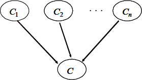

Figure 4.

oel: intersecctionOf.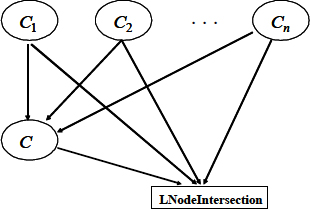

Figure 5.

owl: unionOf.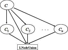

Each primitive or class $C$ (concept) is mapped in variables with two states (true or false) in the Bayesian network.

The constructor “rdfs: subClassO” is modeled by a direct arc node of the parent class (parent superclass) to each node of the subclass son. For example, a concept of class $C$ is defined as a class of the super-concepts $C_{i}$ ( $i=1,\ldots,n$ ) by “rdfs: subClassO”, and it is mapped in a subnetwork in the RB translated, with a connection that converges of each $C_{i}$ to $C$ , as is shown in Fig. 3.

A Class concept of $C$ is defined by the operation of intersection of the classes $C_{i}$ ( $i=1,\ldots,n$ ) using “owl: intersectionOf”, and it is mapped in a subnetwork in the RB translated with a connection that converges of each $C_{i}$ with $C$ , and other connection between $C$ and each $C_{i}$ to a node called LNodeIntersection (see Fig. 4).

A class concept $C$ is defined by the operation of union (owl: unionOf) of the classes $C_{i}$ ( $i=1,\ldots,n$ ), and it is mapped in a subnetwork in the RB translated, with a connection from $C$ to each $C_{i}$ , and a connection of $C$ and each $C_{i}$ to a node called LNodeUnion (see Fig. 5).

If two concepts of class $C_{1}$ and $C_{2}$ are related by any relationship as a complement (owl: complementOf), equivalent (owl: equivalent- Class), or disjoint (owl: disjointWith), then it is created a control node in the Bayesian network and links directed from $C_{1}$ and $C_{2}$ to that node (see Fig. 6).

Based on the previous rules, the RB translated will contain two classes of node. The nodes of regular class for the concepts, and the L-nodes that are nodes associated with the logical relationships. Using the L-nodes, the relationship “rdfs: subClassO” is differentiated from the other logical relationships. Thus, from these relationships are built the CPT of each regular node $C$ . The current implementation of the proposed algorithm in BayesOWL only works for taxonomic ontologies.

Figure 6.

owl: complementOf, owl: equivalentClass, owl: disjointWith.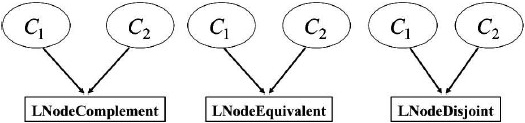

3.2 Construction of the tables CPT

To build the CPTs of the Bayesian Network must be taken into consideration the two types of nodes: the logical nodes (called L-nodes) and the nodes of a concept. The following are the steps for this transformation [21]:

•
CPT for L-nodes (are five types) are specified as follows:

–
LNodeComplement: The relationship complement between $C_{1}$ and $C_{2}$ is calculated as: LNodeComplement is true if $c_{1}\bar{c}_{2}\vee\bar{c}_{1}{c}_{2}$ , otherwise it is false.
–
LNodeDisjoint: The relationship disjoint between $C_{1}$ and $C_{2}$ is calculated as: LNodeDisjoint is true if $c_{1}\bar{c}_{2}\vee\bar{c}_{1}{c}_{2}\vee\bar{c}_{1}{\bar{c}}_{2}$ , otherwise it is false.
–
LNodeEquivalent: The relationship equivalent between $C_{1}$ and $C_{2}$ is calculated as: LNodeEquivalent is true if ${c}_{1}{c}_{2}\vee\bar{c}_{1}\bar{c}_{2}$ , otherwise it is false.
–
LNode Intersection: The relationship $C$ that intersects $C_{1}$ and $C_{2}$ is calculated as: LNodeIntersection is true if $cc_{1}c_{2}\vee\bar{c}\bar{c}_{1}{c}_{2}\vee\bar{c}c_{1}{\bar{c}}_{2}\vee\bar{% c}\bar{c}_{1}{\bar{c}}_{2}$ , otherwise it is false.

•
CPT for the nodes of concept is calculated by ( $C|\pi_{c}$ ), for each variable $C$ of each node of concept in the graph, where $\pi_{c}$ is the set of all parents of $C$ . For that, we follow the next steps:

–
Determine the marginal probability $P$ ( $C$ ) or.
–
Determine the conditional probability ( $C|\pi_{C_{i}}$ ), where $\pi_{C_{i}}\subseteq\pi_{C}$ [21].

The probability distribution for an input $C$ indicates the degree of inclusion of $C$ in its parents, and it is used to fill the CPT, in such a way that is consistent with the probabilistic restrictions in the case, these restrictions may be taken of the ontology and/or learned of the experimental data [21].
4. The autonomic communication system design

4.1 Architecture of our autonomic communication system

The proposed architecture for the implementation is based on the architecture DAISY (see Fig. 1). In particular, in this work are redone the system of recognition of the context and the decision system. The latter system is a separation of the reconfiguring of the system, which consists of two parts, one that makes the decision to reconfigure, and another that sets the protocol of the transport layer, in order to optimize the performance criteria of the communication (i.e., increasing flow, reducing latency, reducing errors, among others). To achieve this goal, one must obtain the traces of the supervised communications system, and calculated from them all performance measures related to Quality of Service (QoS). This is carried out by the monitoring of the Fig. 1.

Figure 7.

Ontology of Shannon and Weaver.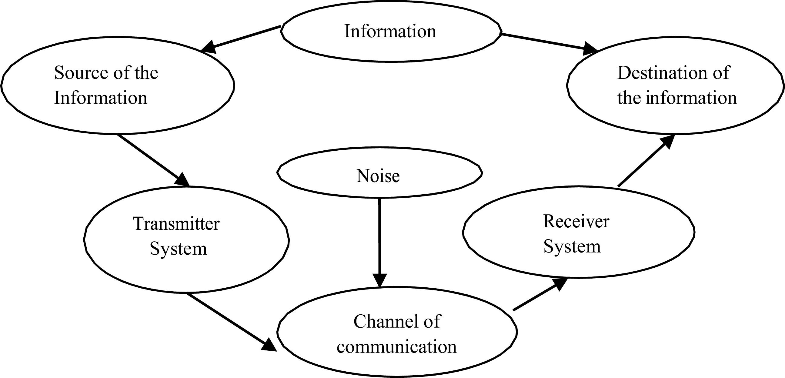

Figure 8.

Ontology for the transport layer [11].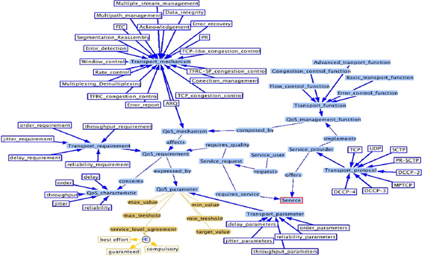

Figure 9.

Ontology of the Hydra project [8].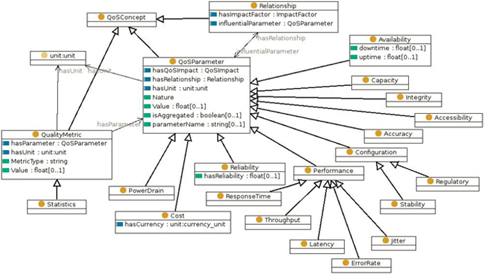

Figure 10.

Ontology of control protocols based on IETF, for the case of multimedia content.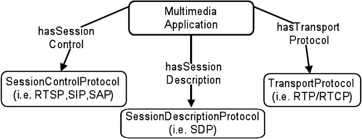

4.1.1 Decision-making system of reconfiguration

This system is part of the system of reconfiguration of the Fig. 1, which is composed of two components: The sub-system of decision of reconfiguration (it takes the decision to reconfigure), and the sub-system for the execution of the reconfiguration (it adjusts the transport layer protocol). The sub-system of decision of reconfiguration (see Fig. 1) is based mainly on a diagram of influence, as the main element for decision-making. It uses the observed patterns in the supervised communication system (these parameters are: flow, delay, rate of losses, among others), which are obtained through the analysis of the traces of communication (subsystem of performance calculation). These parameters also contribute to update the diagram of influence through the learning by counting, in this way the system is updated on the basis of the different experiences that contribute positively with the communication system. In general, the diagram of influence takes the decision whether or not there should be a reconfiguration in the communication system.

4.1.2 System of recognition of context

To build the diagram of influence, this system is composed of the ontology of domain and the Bayesian network. With the ontology, the Bayesian network is built like a previous step to define the diagram of influence. This subsystem monitors the real system, and with its knowledge and the current context, it instances the diagram of influence to make a decision. The ontological characterization is shown in the following sub-section.

4.2 Domain ontology

Domain ontologies are ontologies derived from Metaontologies, which are specific to our system of communication. The ontologies characterize all standards that are used. Below are presented the Meta- Ontologies used in the present work. We start with a general ontology based on the model of Shannon and Weaver (see Fig. 7), which is the model of communications used.

From the model of Shannon and Weaver was defined the ontology to the communication system. However, in this ontology are not taken explicitly into account some aspects, which are described by other ontologies. Some of these aspects are the problems of quality of service, types of protocols, etc., which is important in the modern communication networks. These ontologies are shown in the Figs 8–10. Figure 8 represents an ontology about QoS at the level of the transport layer, it integrates the requirements of applications, mechanisms, functions and protocols of the transport layer, among other things [11]. Figure 9 defines an ontology that represents the quality of service parameters, with criteria of performance, power consumption, capacity, etc. [8]. Finally, Fig. 10 shows an ontology that characterizes the management of multimedia content in communication systems [12]. This ontology is based on the protocols of the IETF (Internet Engineering Task Force), and integrates the section control, the description of the section, and the transmission protocol.

Figure 11.

Performance ontology.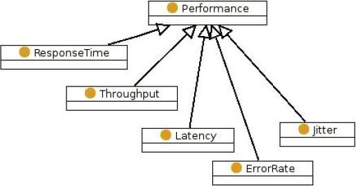

Figure 12.

Proposed ontology.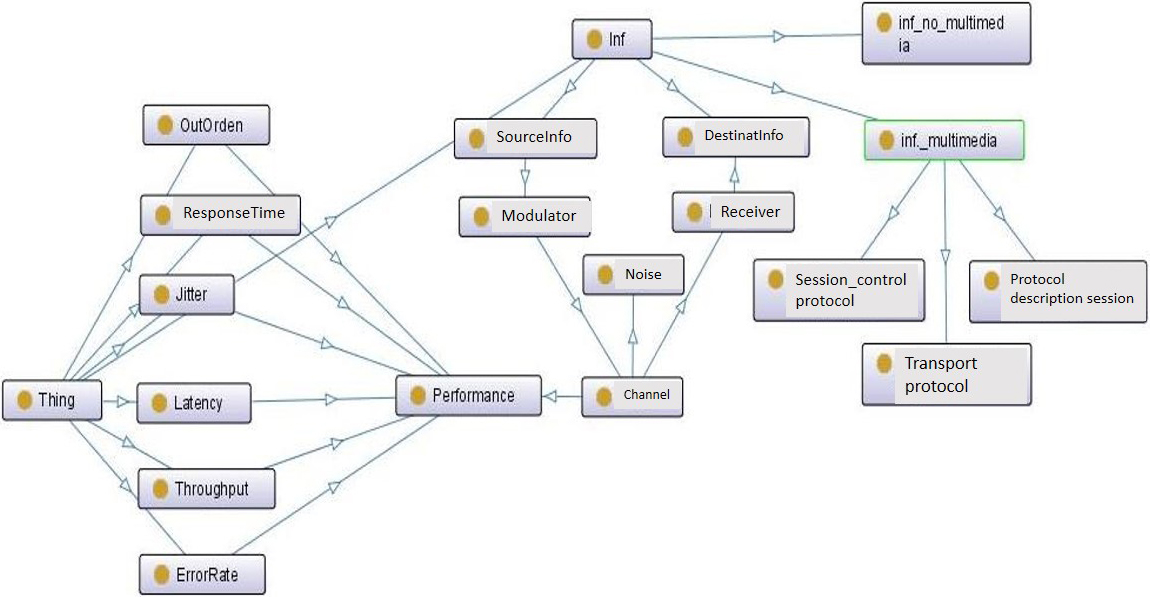

Figure 13.

Reduced ontology.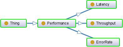

Figure 14.

Primitives class.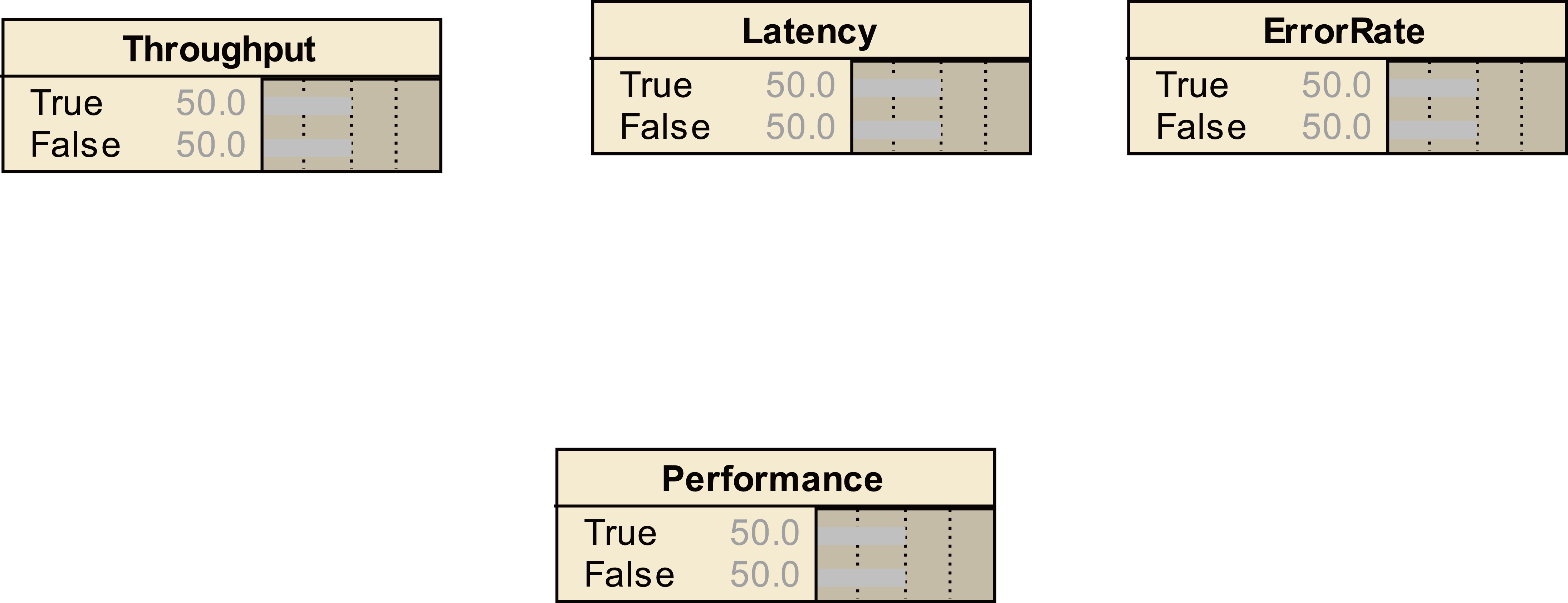

Figure 15.

Subclasses.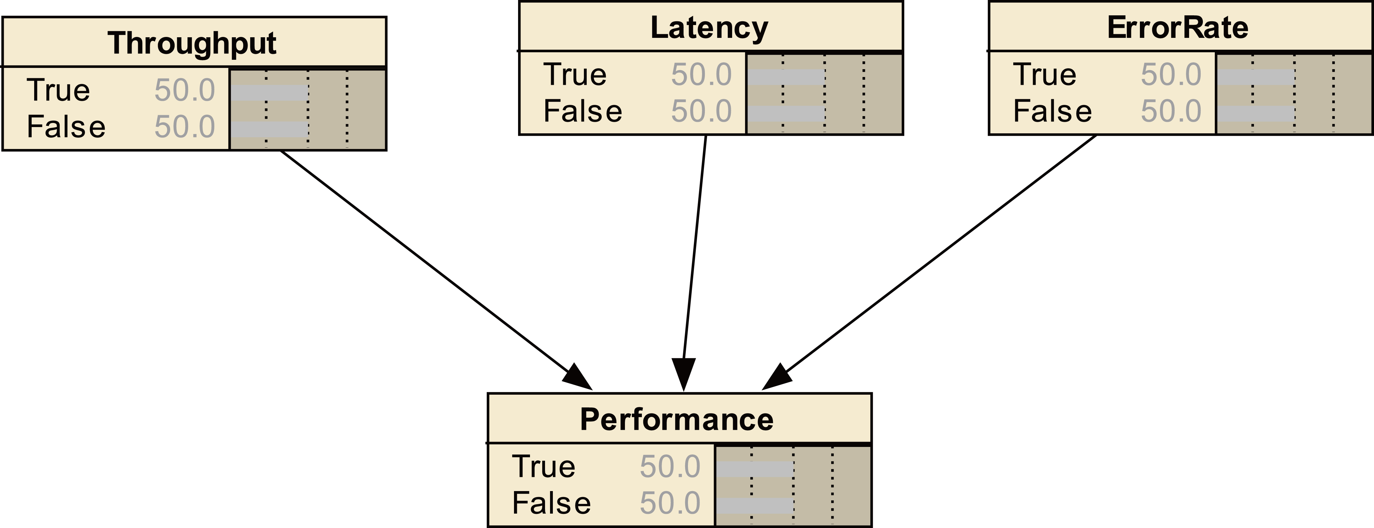

Figure 16.

CPT Tables, with uniform values.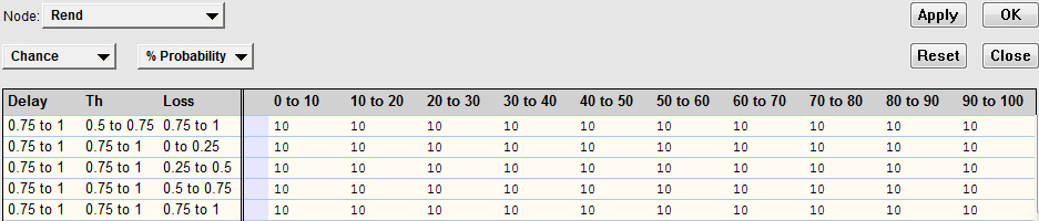

They are now used to form a single ontology that meets the following requirement: to characterize the autonomic communication system. To do this, we analyze each meta-ontology. The relevant elements of the meta-ontologies characterize the QoS parameters, and its ontological relationship with the performance in general of the communication (see Fig. 11). The QoS parameters describe (model) the basic characteristics of the channel of communication, as for example, the delay, the latency, the throughput, among other things.

Now, we need a general meta-ontology that describes the channel, shown in Fig. 7, to which is added the rests of the aspects described in the other ontologies to define the nature of the information to transmit, and the performance parameters. The merged ontology is shown in Fig. 12, and represents a compendium of all the elements used in the autonomous communication networks, taking account the elements involved in the decision-making process.

4.3 Transformation of the ontology to the Bayesian network

To use the previous ontology, we need to transform it into a Bayesian network. For this, the ontology must be described in OWL (BayesOWL structural 1.0) [21].

4.3.1 Transformation of the ontology proposed in Bayesian network

To show the process of transformation, it is considered a fragment of the ontology of Fig. 12 (see Fig. 13). Below are presented each Step of the algorithm:

Structural translation

Step 1: Step 1:
Each primitive or class $C$ concept defined, is mapped in variables with two states (true or false) in the Bayesian network (seeFig. 14).

$<$ owl: Class rdf: ID $=$ “Throughpu”/ $>$

$<$ owl: Class rdf: ID $=$ “Latenc”/ $>$

$<$ owl: Class rdf: ID $=$ “ErrorRat”/ $>$
Step 2:
The constructor “rdfs: subClassO” is modeled by a direct arc from the parent class (parent superclass) to each node of the subclass son. For this, we use the description in OWL (see Fig. 15):

$<$ owl: Class rdf: ID $=$ “Performanc” $>$

$<$ rdfs: subClassOf rdf: resource $=$ “#Throughpu”/ $>$

$<$ rdfs: subClassOf rdf: resource $=$ “#Latenc”/ $>$

$<$ rdfs: subClassOf rdf: resource $=$ “#ErrorRat”/ $>$

Figure 17.
CPT Tables, after of the learning process with EM.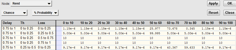

Figure 18.
Ontology with decision node.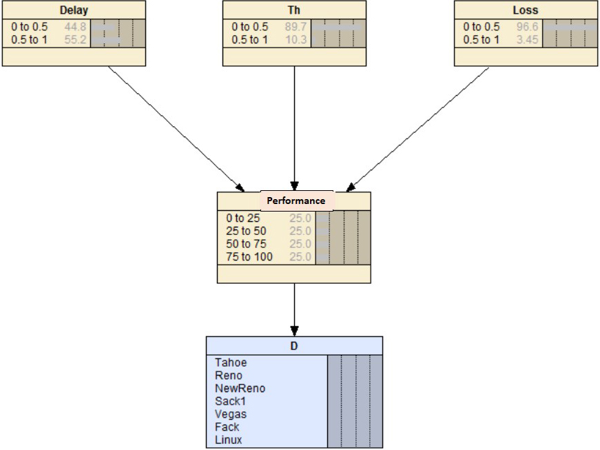

Figure 19.
Ontology transformed into an influence diagram.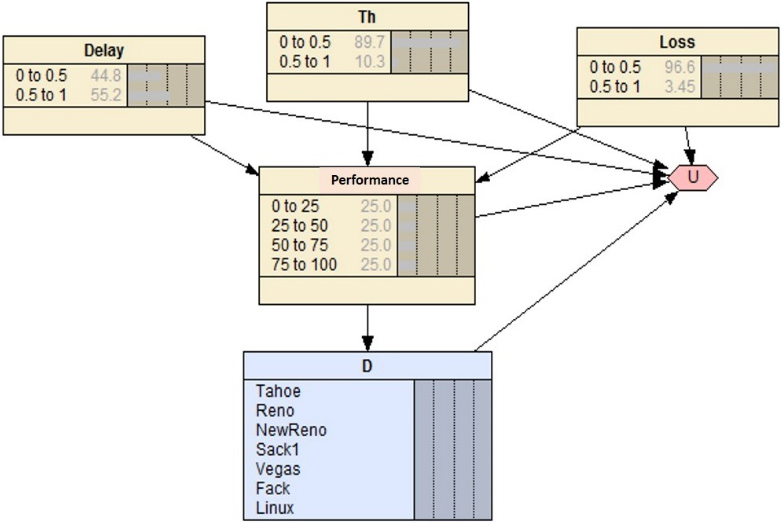

Figure 20.
Influence diagram used for the simulations.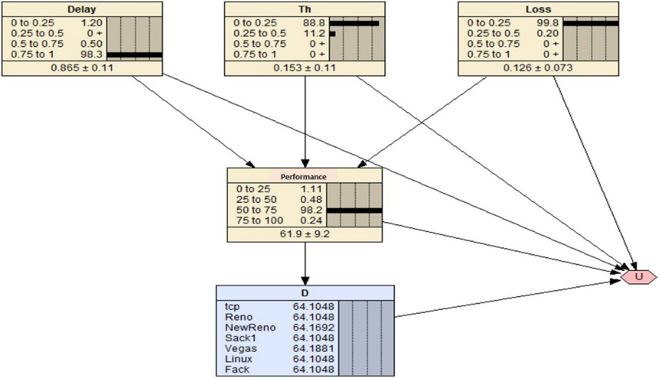

Figure 21.
Utility table at the end of the learning process.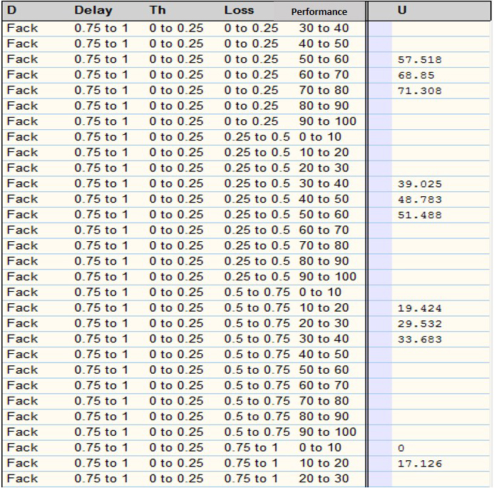

The Steps to create the nodes of operations “owl: intersectionO”, “owl: unionO”, “owl: complementO”, “owl: equivalent-clas”, “(owl: disjointWith)”, do not apply, because the ontology does not use these concepts. Once completed the transformation of the ontology (see Fig. 16), we define the tables CPTs. To build the initial CPTs, we follow the next Steps:

•
Step 1: According to the method of processing of BayesOWL, CPTs can be built from experimental data or ontological restrictions. In this case was calculated from experimental data.
•
Step 2: Multiple experimental simulations are performed.
•
Step 3: After obtaining the experimental data, they are used to calculate the CPTs through the EM learning method. To apply this method, the variables are initialized with random values. In the Fig. 16, we see the initialization of the conditional probability for the performance (Node: rend) variable with respect to different ranges of values of the throughput, error rate and latency variables (the number in each column represents the initial value of this probability in %, for a given number of simulations to be executed).
•
Step 4: The experimental data were used as the current parameters $\theta_{c}^{[t]}$ , to estimate the unknown variables in step E, using the Eqs (3) and 4. Then, the algorithm goes to the step M (see the detailed procedure with the steps E and M in the Section 2.2: Learning by method of maximizing the expectation), where it is calculated the Eq. (5) in the table. The steps E and M are repeated to stabilize the estimated values. At the end of the learning, the initial values in the CPTs are modified by the results of this phase (The values in the columns represent the final value of the conditional probability of the performance variable in %, for a given number of simulations and different combinations of the input variables).

4.4 Transformation of the Bayesian network in a diagram of influence

Now, the Bayesian Network must be transformed into a diagram of influence, in order to use the criterion of MUE, and thus facilitate the decision making in the system. In this paper, the idea is that the system decides what type of reconfiguration must be executed to maximize the performance of the communication. In the node of decision must be placed the alternatives of change that are presented. This process begins with the ontology of the Fig. 15, and adds the nodes of decision, as is shown in Fig. 18. In our case, there is a single node of decision, in this node of decision will be coded all possible changes that can be made according to the context in which it is going to use.

Once decision nodes are created, we proceed to create the utility function (table of utility). This table is displayed as a node (node of utility) with dependence with all nodes with which that table of utility has a relationship (see Fig. 19).

4.5 Learning process

With the diagram of influence obtained (Fig. 19), it is necessary to characterize the node of utility with the experimental data obtained from multiple simulations for different values of parameters (delay, capacity of the channel, and rate of loss). Figure 20 shows the influence diagram used for the simulations of the communication system with NS2. Figure 20 shows that the values for the variables delay (Delay), Flow (Th), performance and rate of losses (Loss) are divided into four ranges of values, this is due to the type of dispersion of the experimental data, which was not easily describable with less ranges. These ranges are assigned by means of a frequency distribution. This distribution of frequency depends on the simulations, and may change.

The table of utility has the following characteristics: it is defined by the node of utility $U$ of the diagram of influence of the Fig. 20, which depends, in this case, of all the variables of the diagram of influence (Delay, Flow (Th), performance and rate of losses (loss)) and the node of decision ( $D$ ).

The initial learning process was conducted using the EM technique on the Bayesian network; after this initial learning, the system continues the learning process using the counting-learning method. This second learning process is carried out after each decision of reconfiguration. This process reinforces the Bayesian network, so that the decisions that increase the performance of the system also will help to improve the system of decision. This process consists in update the Bayesian network and the table of utility, so that the system can improve its performance.

In Fig. 21, we can see the table of utility after the process of learning. The utility is calculated using the Eq. (14), using the observed data in the system of the delay, flow (Th), loss variables, and in particular, the performance, which also depends on all of the above. The decision-making model seeks to optimize the maximum expected utility in the performance:

$\displaystyle U=\textit{MAX}(\textit{Performance})$ (14)

While the system learns in the initial stage, it does not take any decision. At the end of this stage, the system takes decisions on the basis of the table of utility, choosing the greatest possible utility in the table for a given input.

5. Experiments

To verify the behavior of the decision system built from the ontology proposal, we use the NS2 simulation tool [20]. In addition to the NS2 simulator, we use APIs for networks of beliefs (Bayesian networks) and influence diagrams of the company NORSYS (in particular, the software netica) [19], to implement the decision system of our autonomic communication system.

5.1 Design of the experimental protocol

We have implemented a script, called parametric (simulation script), which changes online the parameters of the simulation in NS2, depending on the decisions taken by our decision system. The decision system uses as input, the analysis of traces of the simulation. Once obtained the traces of the simulation, are analyzed by using a script that determines the results of the Simulation: flow rate, rate of loss and delay. With these variables, the decision system determines the reconfigurations in the simulation to improve the communication performance. Then, the simulator runs again with the new reconfiguration.

Table 1
Example of the results of a simulation

Rate of loss	Performance		Throughput		Changes: (when/new TCP)
	Without SA	With SA	Without SA	With SA
25%	38,26	43,92	0,003563	0,005179	24,001147/(from TCP/Linux to TCP/Sack1)

Table 2

Results of the simulations for different scenarios

Diagram of	Scenario	Number of	Number of simulations	Number of simulations	Number of simulations
influences		simulations	with changes	with better performance	with better flow rate
Type 1	Var. of the packet loss	19	10	9	6
	Var. of the Bandwidth	10	4	4	4
	Var. of the delay	10	6	6	6
	Var. of the congestion	8	6	5	6
	Total	47	26 (55.3%)	24 (92.3%)	22 (84.6%)
Type 2	Var. of the packet loss	19	8	7	7
	Var. of the Bandwidth	10	4	4	4
	Var. of the delay	10	6	6	6
	Var. of the congestion	8	6	6	6
	Total	47	24 (51%)	23 (95.8%)	23 (95.8%)

Figure 22.

Performance with and without autonomic system.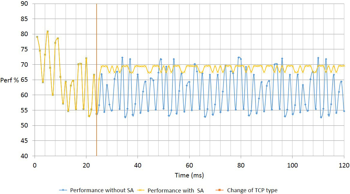

Figure 23.

Throughput with and without autonomic system.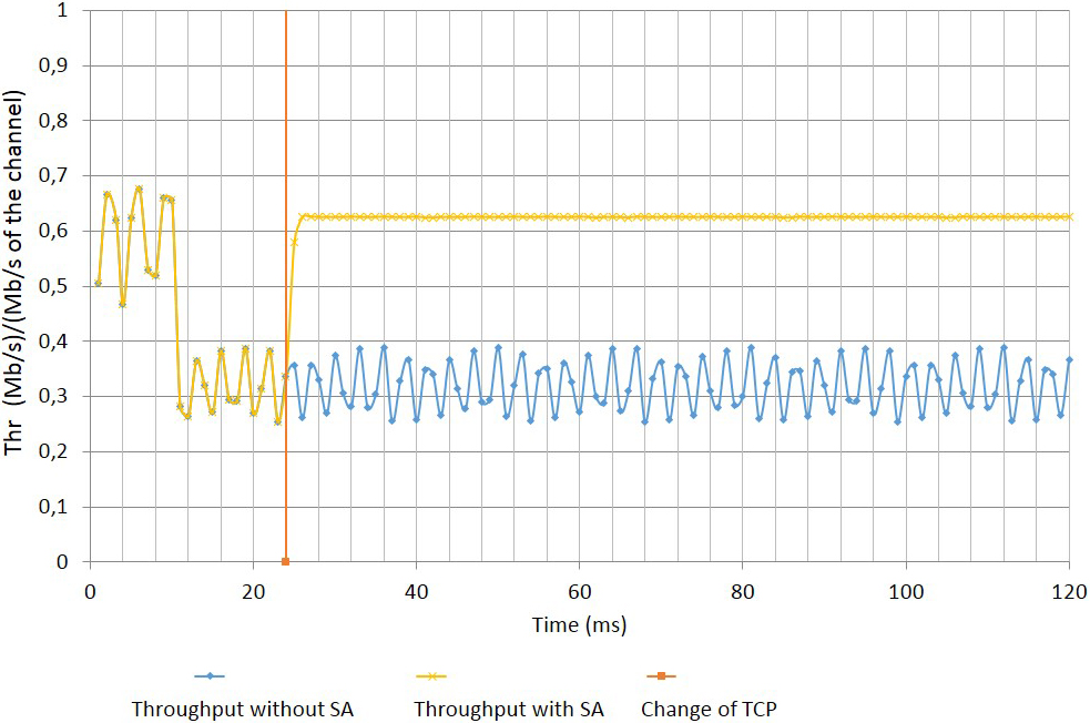

To calculate the flow rate, the rate of losses and the delay, we use a script that takes into consideration the amount of packets that are received successfully, that are sent, which are discarded, and the time in which they were sent and received. With these three parameters we use the following equation, based on a proposal in [26], inspired by the parameters of an ideal communication, to calculate the performance.

$\displaystyle\textit{Performance}{=}\sqrt{\frac{\textit{DelayR}^{2}+\textit{% FlowN}^{2}}{2}}(1-\textit{Tloss})$ (15)

These variables have been defined in [26] as nominal values between 0 and 1, to indicate that a value of 100% of performance (1) means that the communication is ideal. The DelayR is the relative delay, normalized linearly with a theoretical delay (Rt), following the proposed in [26]. The FlowN is the Normalized Flow to the maximum that can be obtained in the simulation due to the minimum bandwidth on the path, which represents the maximum flow rate that can reach the desired communication. Tloss is the loss rate, is the ratio between the number of packets lost and the total number of packets sent.

The sub-system for the calculation of performance invokes the diagram of influence when it determines that a decision must be made, which is when there is a degradation in performance.

5.1.1 Simulation process

Due to the limitations in the form as is built the NS2 simulator, cannot be modified the parameters in real time. For this reason, in our experimental platform the decision system takes the decision to reconfigure offline. In addition, therefore, also it is launched a new simulation with the new configuration caused by the decision of our system, and it is compared with the initial simulation. In this way, we can determine if the decision taken by the decision system increase the performance. An example of comparison, for a scenario with a rate of loss of 25%, of the simulation with and without changes, can be seen in Table 1. In general, the performance and throughput averages of our approach are lower, once our decision system proposes changes; it decides to change at the time 24,001147 ms from TCP/Linux to TCP/Sack1. The graphics about the performance and throughput for the simulation of the Table 1, may be observed in the Figs 22 and 23, respectively.

In Fig. 22, we can see the result of two simulations: the first is the performance without autonomic system (SA), and the second is the performance with SA, when SA took the decision to reconfigure at the time 24.001147 ms (changes TCP/Linux to TCP/Sack1). We see an increase in the performance average of 38.26% to 43.92%. With respect to Fig. 23, the throughput is observed with and without SA, for the same simulation of Fig. 22. There, clearly shows that after 24 ms is better the throughput of the SA.

5.1.2 Experimental protocol

In this section, we define different scenarios. The scenarios used are:

•
Scenario with a variation of the packet loss: In this scenario will vary the rates of loss during the simulation.
•
Scenario with a variation of the Bandwidth: In this scenario will vary the bandwidth of the channel during the simulation.
•
Scenario with a variation of the delay: In this scenario will vary the delay during the simulation.
•
Scenario with a variation of the congestion: In this scenario will vary the type and rate of transmission of the packets during the simulation.

Table 3
Improvements according to the Type of diagram of influence

Influence Average of the Average of the

diagram flow rate with SA performance with SA

Type 1 62.60% 1.60%

Type 2 66.35% 1.95%

Figure 24.
Diagram of influences.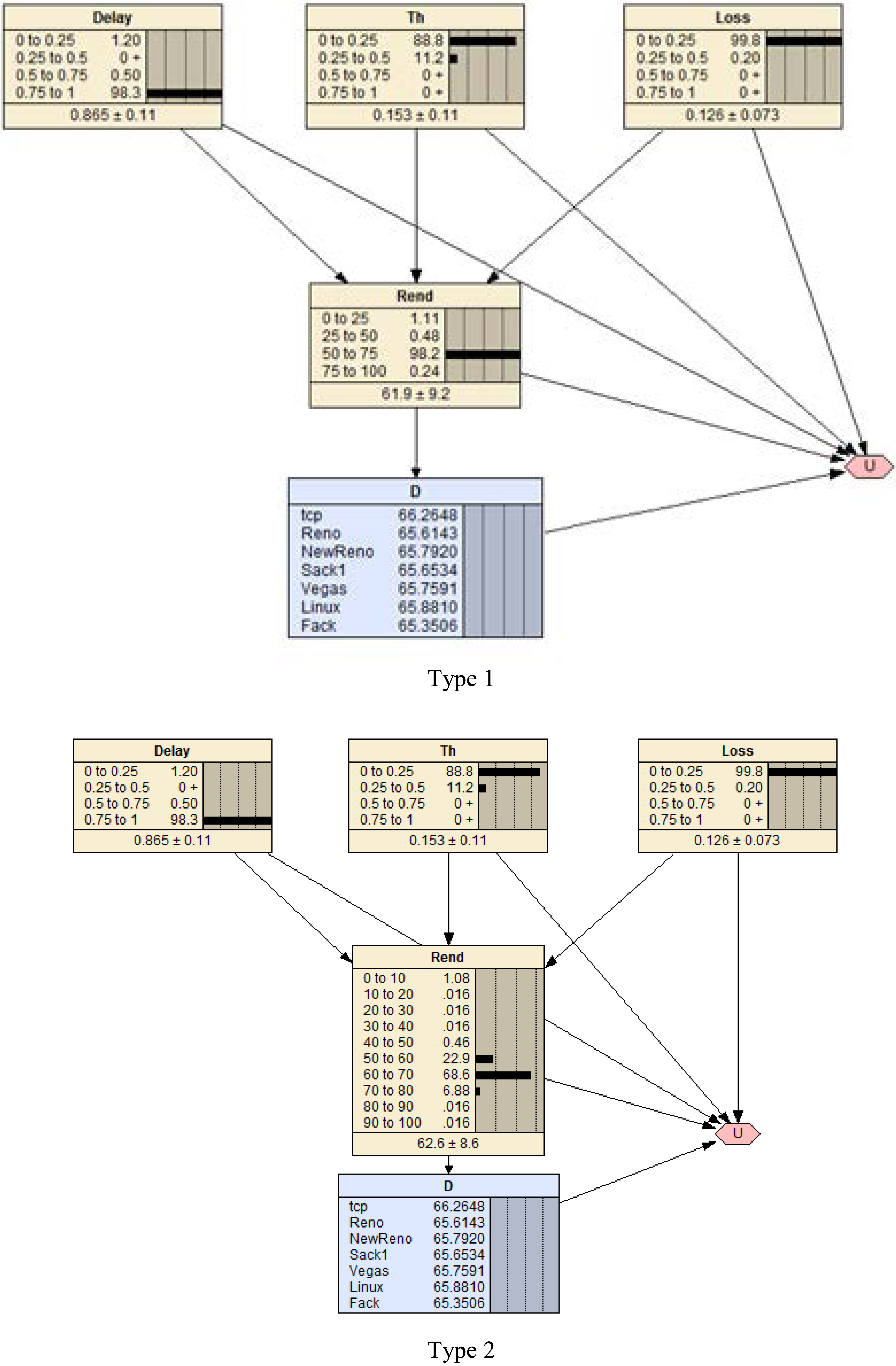

In each scenario, we have used an exponential distribution for the variation of each variable. Additionally, we define two influence diagrams, they differ in the number of ranges used to describe the performance variable (see Fig. 24). The main reason of these influence diagrams is to test if the number of performance states in the system can distinguish a greater number of situations, in order to take better actions.

Table 4
Utility results due to the l

Initial $U$ after the training $U$ at the end of the simulations Conditions of the variables in the simulation

value phase (learning by EM) (learning by count) D Delay Th Loss Rend.

0 52.455 55.501 Linux 0.5 to 0.75 0.25 to 0.50 0 to 0.25 50 to 60

0 47.065 47.363 Fack 0.5 to 0.75 0.5 to 0.75 0 to 0.25 50 to 60

0 50.569 50.926 Reno 0.75 to 1 0 to 0.25 0.25 to 0.5 50 to 60

0 51.035 53.422 Linux 0.75 to 1 0.5 to 0.75 0 to 0.25 60 to 70

Table 5
Comparison between different works

Attribute Our work [26] [20]

Knowledge base Ontology and Bayesian network Bayesian network Bayesian network

Predictive capacity If, through the Bayesian network Has not If, through the Bayesian network

Evaluation of Comparison between the control system Only quality of service QoS Comparison between the control

performance without autonomic system and autonomic system, and quality of service goals system without autonomic system and autonomic system

Mechanism of action Change the transport protocol Change the transport protocol Change the router

Adaptive mechanism Learning No defined learning mechanism Learning

Implements a closed Based on the DAISY architecture Not Not

loop (MAPE)

Self-managed Yes Not Yes

Figure 25.
Scenario with different loss rates.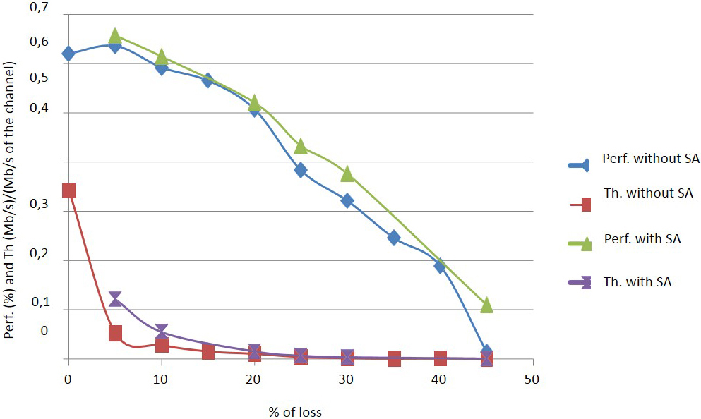

In each scenario, the system takes the decision based on the variable that is varying. The results are shown in Table 2. In the case of the diagram of influences Type 1, our autonomic system makes changes in the 55.3% of the cases. For these cases, the performance improved in the 92.3% of these cases, and the flow rate in the 84.6% of these cases. For the simulations with the diagram of influence Type 2, our autonomic system makes changes in the 51% of the cases. In the 95.8% of the cases where our autonomic system makes changes, the rate of flow and performance are increased. Our autonomic system always improves the results for the case of variation of the bandwidth and delays. In few cases, the changes of our autonomic system don’t improve the performance and flow rate. Sometimes, the system does not take decisions due to the current conditions of the communication system, which the autonomic system considers is ok.

Finally, Table 3 shows the average of the improvements in the two Types of influence diagrams. The average of improvement in performance is 1.95%, and in flow rate is 66.35%, for Type 2, which is better that for Type 1.

In general, the results of the diagram of influence Type 2 are better because the decision system has different levels of performance to characterize the context. That is, a larger number of states are effective, but the table of utility grows significantly (for this example, from 1792 to 4480 entries). Our autonomic system improves the communication due to the influence diagrams, which characterize the different communication protocols based on their performance characteristics (rate of loss, delay, etc.). In this way, our autonomic system takes decisions that improve effectively the communication.

Now, we carry out simulations in the scenario where is changed the rate of packet loss only for the influence diagram Type 2, using the autonomic system and without it. Figure 25 shows the results. The Fig. 25 in the Y axis shows two variables, performance (perf) and traffic flow (th), to compare our proposal (SA) with the fact of not using it for the management of the communication system. In addition, in the case of our proposal, we begin to show its results after the rate of loss begins to change, since at the beginning when there are not changes in it, it is not interesting its utilization (SA must not carry out any adaptation in the communication system). The curve of “with SA” is above to the curve of “without SA”. Due to the changes proposed by our system, the flow and the performance are improved considerably. The ability of the system to carry out several changes dynamically, demonstrates its flexibility.
5.2 Results of the learning process

Influence	Average of the	Average of the
Type 1	62.60%	1.60%
Type 2	66.35%	1.95%

Initial	$U$ after the training	$U$ at the end of the simulations	Conditions of the variables in the simulation
value	phase (learning by EM)	(learning by count)	D	Delay	Th	Loss	Rend.
0	52.455	55.501	Linux	0.5 to 0.75	0.25 to 0.50	0 to 0.25	50 to 60
0	47.065	47.363	Fack	0.5 to 0.75	0.5 to 0.75	0 to 0.25	50 to 60
0	50.569	50.926	Reno	0.75 to 1	0 to 0.25	0.25 to 0.5	50 to 60
0	51.035	53.422	Linux	0.75 to 1	0.5 to 0.75	0 to 0.25	60 to 70

Attribute	Our work	[26]	[20]
Knowledge base	Ontology and Bayesian network	Bayesian network	Bayesian network
Predictive capacity	If, through the Bayesian network	Has not	If, through the Bayesian network
Evaluation of	Comparison between the control system	Only quality of service QoS	Comparison between the control
performance	without autonomic system and autonomic system, and quality of service goals		system without autonomic system and autonomic system
Mechanism of action	Change the transport protocol	Change the transport protocol	Change the router
Adaptive mechanism	Learning	No defined learning mechanism	Learning
Implements a closed	Based on the DAISY architecture	Not	Not
loop (MAPE)
Self-managed	Yes	Not	Yes

A sample of the quality of learning on the utility ( $U$ ) is shown in Table 4. The value of $U$ (Utility) is improved according to the system learns. In that table, each row is a different simulation. For example, in the first row, the first column is the initial value of $U$ . Then, the next column is the utility value at the end of the first phase of learning (52.455, learning by EM). After that period, the system begins to take decisions and continues to learn (learning by count). At the end of the simulations (second phase of learning), the value of $U$ is 55.501. In all the cases of the Table 4, the learning process improves the utility ( $U$ ), it is a fundamental component of our autonomous system.

5.3 Comparison

In this section, we compare our autonomous communications system with previous works. We carry out a qualitative comparison, based on the proposed design reported in the literature for each one of these works. The criteria were if they use a knowledge base for the decision making, if they have the ability to predict the future state of the communication system, how to evaluate its quality, which are the adaptive mechanisms and actions perform in the communication system, and if they propose an autonomic model (based on the MAPE paradigm) for the self-management [28]. Particularly, the MAPE paradigm establishes that all autonomic system has a closes loop composed by the next set of tasks: to monitor and to analysis the current situation in the system, to plan the next set of actions in the system according to the conclusions in the previous tasks, and finally, to execute these actions on the system [28]. In Table 5, we define this set of attributes, which are interesting for designing autonomic systems.

Our approach accomplishes all of them. In the case of [26], it does not present learning and MAPE mechanisms. In the case of [20], they have not MAPE mechanism, and the metrics used are very limited (we use an ontology that can be extended), and should be improved so that its decision-making process more efficient.

6. Conclusions and recommendations

We have proposed an autonomic communication system based on Bayesian Networks and ontologies, which is inspired by the DAISY architecture. The ontology defines the different standard used currently, which serves as basis for building the Bayesian network, which is the essential part of the decision-making system. The performance of our SA is satisfactory, improving the communication in general. We have tested the capabilities of the system in multiple scenarios, demonstrating its capabilities of adaptation and learning. The system developed has, among others, the capacity for self-optimization, which is mainly reflected in the learning process that is performed in the Bayesian network and the table of utility. Both components are modified according to the experience of the SA.

Our approach offers several improvements over previous works [26, 20]: all the parameters needed to analyze the current situation in the communication system (flow rate, loss rate, delay) can be determined by observing the communication from the emitter. Additionally, the system proposes an adaptive process of decision-making (Bayesian Network). Finally, the system is based on an ontology, which contains the basic standards used in this domain, by giving great conceptual robustness at the same. Another advantage of our system is the low computational cost, since none of the algorithms used has a computational cost greater than a linear function, which contributes positively in its future implementation.

Future works will carry out an exhaustive analysis of our SA approach for multi-variation cases, in different contexts of communication networks, such as wireless personal communication networks, local area networks, wide area networks, satellite networks and metropolitan area networks. Additionally, our SA approach will be extended with the concept of autonomic cycle of data analytical tasks [4], in order to include specific analysis tasks in our system linked to improving the quality of services, among other aspects, using the data.

Footnotes

Acknowledgments

Dr Aguilar has been partially supported by the Prometeo Project of the Ministry of Higher Education, Science, Technology and Innovation of the Republic of Ecuador.

References

Aguilar

, Definition of an energy function for the random neural to solve optimization problems, Neural Networks 1 (1998), 731–737.

Aguilar

Subias

Travé-Massuyés

and Zouaoui

, Situation Assessment in Autonomous Systems, Proceedings of the 4th Global Information Infrastructure and Networking Symposium, IEEE Communication Society, 2012.

Aguilar

Jerez

Exposito

and Villemur

, CARMiCLOC: Context awareness middleware in cloud computing, Proc Latin American Computing Conference (CLEI) (2015), 1–10.

Aguilar

Buendia

Moreno

and Mosquera

, Autonomous cycle of data analysis tasks for learning processes, in: Technologies and Innovation, Communications Computer and Information Science Series Valencia-García

et al., eds, Springer 658 (2016), pp. 187–202.

Aguilar

Torres

and Aguilar

, Autonomic decision making based on bayesian networks and ontologies, Proc IEEE International Joint Conference on Neural Networks (2016), 3825–3832.

Bencomo

and Belaggoun

, Supporting decision-making for self-adaptive systems: From goal models to dynamic decision networks, Lecture Notes in Computer Science 7830 (2013), 221–236.

Ben-Gal

I.F.

Faltin

and Kenett

, Bayesian Networks, Encyclopedia of Statistics in Quality & Reliability, Wiley & Sons, 2007.

Consortium

, D4.10 Quality-of-Service Enabled Hydra Middleware, 2009.

Crowley

, Evaluating influence diagrams where we’ve been and where we’re going, British Columbia: University of British Columbia, 2004.

10.

Dobson

Massacci

and Denazis

, A survey of autonomic communications, ACM Transactions on Autonomous and Adaptive Systems 1(2) (2006), 223–259.

11.

Exposito

, Méthodologie modèles et paradigmes pour la conception d’une couche transport de nouvelle génération, Toulouse: LAAS-CNRS, 2010.

12.

Exposito

Lamolle

and Gómez-Montalvo

, Introducing an ontology driven architecture for distributed, Proc 2010 Second International Conference on Information, Process, and Knowledge Management (2010), 7–12.

13.

Ghahramani

, The Handbook of Brain Theory and Neural Networks, in: Graphical models: parameter learning Arbid

, eds, MIT Press, 2003, pp. 486–490.

14.

Helspe

E.M.

and van der Gaag

L.C.

, Building Bayesian networks through ontologies, Proc 15th European Conference on Artificial Intelligence (2002), 680–684.

15.

Hudec

and Fenz

, Ontology-based generation of Bayesian networks, Proc International Conference on Complex, Intelligent and Software Intensive Systems (2009), 712–717.

16.

IBM, An architectural blueprint for autonomic computing, New Tork: IBM. IETF, Internet Engineering Task Force, https://tools.ietf.org/html/rfc1122 (2005).

17.

Kephart

and Chess

, The vision of autonomic computing, IEEE Computer Society 3 (2003), 41–50.

18.

Kjaerulff

U.B.

and Madsen

A.L.

, Bayesian Networks and Influence Diagrams, Aalborg Denmark: Springer, 2005.

19.

Norsys

S.C.

, Netica API Programmer’s Library Reference Manual Version 4.18, Vancouver, BC, Canada: Norsys Software Corp, 2010.

20.

Zhang

Cao

Sun

and Tan

, Cognitive networks autonomic decision-making approach based on influence diagram, Journal of Networks 7(5) (2012), 876–883.

21.

Rong

Zhongli

and Peng

, A bayesian network approach to ontology mapping, Baltimore, Maryland, USA, 2006.

22.

Rong

Zhongli

and Peng

, BayesOWL: Uncertainty modeling in semantic web ontologies, Soft Computing in Ontologies and Semantic Web Studies in Fuzziness and Soft Computing 204 (2006b), 3–29.

23.

Dobson

Denazis

Fernández

Gaïti

Gelenbe

Massacci

Nixon

Saffre

Schmidt

and Zambonelli

, A survey of autonomic communications, ACM Transactions on Autonomous and Adaptive Systems 1(2) (2006), 223–259.

24.

Sucar

, Redes Bayesianas, in: BS Araujo, Aprendizaje Automático: Conceptos básicos y avanzados, Pearson Educación, 2006, 77–100.

25.

Tenenbaum

Griffiths

and Kemp

, Theory-based Bayesian models of inductive learning and reasoning, TRENDS in Cognitive Sciences 10(7) (2006), 309–318.

26.

Van

, PhD Thesis: Une approche pour la composition autonome de services de communication orientés QoS. Application aux protocoles de transport configurables, Toulouse: Mathématiques Informatique Télécommunications de Toulouse (MITT), 2009.

27.

Vizcarrondo

Aguilar

Exposito

and Subias

, ARMISCOM: Autonomic reflective middleware for management service composition, Proc Global Information Infrastructure and Networking Symposium (GIIS) (2012), 1–8.

28.

Vizcarrondo

Aguilar

Exposito

and Subias

, MAPE-K as a service-oriented architecture, IEEE Latin America Transactions 15 (2017), 1163–1175.

29.

Zaragoza

J.H.

Sucar

and Morales

E.F.

, A two-step method to learn multidimensional Bayesian network classifiers based on mutual information measures, Proc Twenty-Fourth International Florida Artificial Intelligence Research Society Conference (2011), 644–649.

30.

Gómez-Montalvo

, MODA: A multimedia ontology-driven architecture for autonomic quality of service management in home networks, PhD Thesis, LAAS-CNRS, 2012.

31.

Howard

R.A.

and Matheson

J.E.

, Influence diagrams, in: Readings on the Principles and Applications of Decision Analysis Howard

R.A.

and Matheson

J.E.

, eds, Vol. II, Strategic Decisions Group, Menlo Park, California, 1981, pp. 719–762.

Influence	Average of the	Average of the
diagram	flow rate with SA	performance with SA
Type 1	62.60%	1.60%
Type 2	66.35%	1.95%

Autonomic communication system based on cognitive techniques

Abstract

Keywords

1. Introduction

1.1 Research background

1.2 Literature review

1.3 Paper positioning

2.1 Autonomic communication systems

Learning by method of maximizing the expectation

• Represent information of OWL as probabilities. • Translate OWL ontologies to RB. – Rules to build the structure of the RB from triplets OWL. – Help for the addition of special nodes for the logical relationships. – Construction of tables CPT. 3.1 Structural translation

4.1 Architecture of our autonomic communication system

4.1.2 System of recognition of context

4.2 Domain ontology

4.3.1 Transformation of the ontology proposed in Bayesian network

Structural translation

4.5 Learning process

5.1 Design of the experimental protocol

Table 1 Example of the results of a simulation

5.1.2 Experimental protocol

5.3 Comparison

6. Conclusions and recommendations

Footnotes

Acknowledgments

References

•
Represent information of OWL as probabilities.
•
Translate OWL ontologies to RB.

–
Rules to build the structure of the RB from triplets OWL.
–
Help for the addition of special nodes for the logical relationships.
–
Construction of tables CPT.

3.1 Structural translation

Table 1
Example of the results of a simulation