Assessment of open-pit captive limestone mining areas using sentinel-2 imagery with spectral indices and machine learning algorithms

Abstract

Limestone mining is a significant economic activity in India, accounting for around 10% of the GDP however, it has certain negative environmental consequences. The objective of this study is to determine the spatial distribution area of captive limestone mines using remote sensing datasets, spectral index, and machine learning algorithms and compare their area estimation with industrial field survey reports for the financial year 2019. The study area includes a limestone resource area of 2226.16 ha with an excavation area of 487.10 ha in 2019. In the present research, we used a high-resolution Sentinel-2A satellite dataset to map and compute the active mining area by implementing the Normalised Vegetation Index (NDVI), Iterative Self-Organizing Data Analysis Technique (ISODATA), K-Nearest Neighbours (KNN), and Random Forest (RF) algorithms in the QGIS 3.18 software tool. The RF classifier estimated a limestone mine area of 379.57 ha with user accuracy (UA) of 97.25% and producer accuracy (PA) of 99.18% with a kappa coefficient value of 0.957. The mine area was estimated at 417.47 ha with a UA of 98.99% and PA of 99.10% and kappa value of 0.947 of the KNN method, The NDVI method estimated 469.92 ha with a UA of 93.63% and PA of 92.04% and kappa value 0.685. This research confirmed that the RF classifier well performed in classification with overall accuracy (OA) of 95.79% to KNN (OA of 94.78%), NDVI (OA of 79.84%) classifiers, and ISODATA poor in classification with OA of 64.16%. This research assists limestone mine owners and environmental engineers in making environmentally sustainable decisions, eco-friendly mine design, and monitoring.

Keywords

Limestone mine multispectral image machine learning NDVI

1. Introduction

Limestone is a sedimentary rock mainly made of calcite (CaCO ${}_{3}$ ). Limestone often contains considerable amounts of dolomite (CaMg(CO ${}_{3}$ ) ${}_{2}$ ) as well as minor constituents of clay, iron carbonate, silica so on (https://geology.com/). Limestone is the primary raw material used in the manufacturing of cement, in the construction industry for building walls and floors, and as a flux in the metallurgical sector (www.mines.ap.gov.in). Limestone of high quality is used in the chemical, sugar, paper, glass, alkaline, leather, and tanning industries. India is rich in high-quality limestone reserves. According to NMI (National Mineral Inventory), data based on the UNFC (United Nations Framework Classification) system, India’s total cement-grade limestone reserve available in 2015 is approximately 203,224 million tonnes, of which 16,336 million tonnes (8%) are categorized as reserves and 1,86,889 million tonnes (92%) as resources [1].

The Yerraguntla cement industrial region is a prominent cement producer in the YSR Kadapa district of Andhra Pradesh, India. The region is endowed with extensive deposits of cement-grade limestone (calctufa) over an area of approximately 2226.16 ha with an excavation mining area of 487.10 ha in 2019 [2]. The amount of limestone produced in India during the 2019 fiscal year was close to 380 million metric tons [1]. The destruction of the environment brought on by limestone extraction in terms of dust and noise leads to geomorphological issues that have a significant impact on human civilization and existence at local levels [3].

Nowadays, machine learning applications in remote sensing are a trending topic that is gradually gaining attention from industry experts, scientists, and researchers [4] due to the availability of modern techniques in remote sensing, abundant data availability, and, when compared to traditional ground-based mapping techniques, spatial remote sensing has indisputable benefits in terms of covered area, speed, and cost [5]. Remote sensing technology benefits from machine learning techniques as they enable better resource management, more accurate environmental forecasts, and the discovery of novel insights from large data sets. While there are many benefits to using machine learning in remote sensing, there are some challenges as well. The availability of up-to-date data, the development and validation of training data, and algorithm design uncertainty are all barriers to machine learning being widely used [6]. The objectives of the research as follow (1). To map open-pit captive Limestone mining area in the study area using spectral index and machine learning algorithms; (2). To assess and compare the mining area with industrial field survey data; (3). Classifier performance evaluation in the mapping and appraisal of limestone mining areas;.

This article is organized as follows: Section 1 presents an overview and objectives of the research; Section 2 discusses a literature review of lithological mapping techniques; Section 3 presents materials and methods relevant to the limestone mining region, including data collection, preprocessing, and digital classification; Section 4 presents the findings and discussion; and Section 5 provides the conclusions of the study.

2. Literature review

Wang et al. [7] incorporated multi-sensor and multisource remote sensing images and used a hybrid classification method of Metric Learning (ML) and Random-Forest (RF) to differentiate major lithological units in the Himalayan orogenic belt, promoting computing efficiency and 85.75% overall classification accuracy [8]. Bachri et al. [9] used the RF method to map lithological characteristics utilizing Sentinel-2A (MSI) spectral, textural, and geomorphic information with the ALOS PALSAR. The results revealed that the RF approach is a good tool for creating new geological maps or updating existing ones, with a kappa hat of 0.88 and an overall accuracy of 91%. Shirmard et al. [4] explored high-capability RS datasets and machine-learning algorithms for mapping various geological features such as rock types, structures, and mineralized zones. Abdolmaleki et al. [10] used a support vector Machine (SVM) and combined remote sensing and geological data to generate a mineral prospectivity map. Davids and Rouyet [11] evaluated various remote sensing approaches that can be employed for mining-related applications such as surface mineralogy mapping for development, topographical changes used during mine design and operation, environmental consequences monitoring, and mapping surface motions of mine structures. El Atillah et al. [12] used ISODATA and Kinetic Monte Carlo (KMC) methods to perform lithological cartography. The integration of structural, lithological, and hydrothermal alteration data gathered from ASTER, Landsat (ETM $+$ and OLI), and Sentinel-2A data offered an overview of the mineralogy of the studied area. The findings were evaluated and compared to field data and geological maps from the study region. Rahman et al. [13] assessed rural and urban extents using Random Forest and Support Vector Machine (SVM) algorithms on Landsat-8 and Sentinel-2 images, with an overall accuracy of 96.9%, 98.3%, and kappa values of 0.948 and 0.968, respectively.

3. Materials and methods

3.1 Study area

Figure 1.

Location of limestone mines in the cement industrial area at YSR Kadapa district.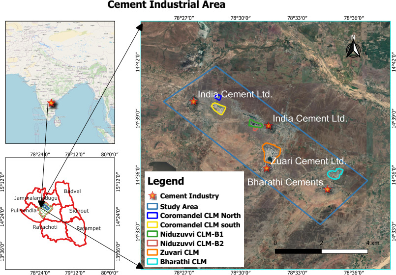

Figure 2.

Classification and performance evaluation of classifiers in limestone mine mapping.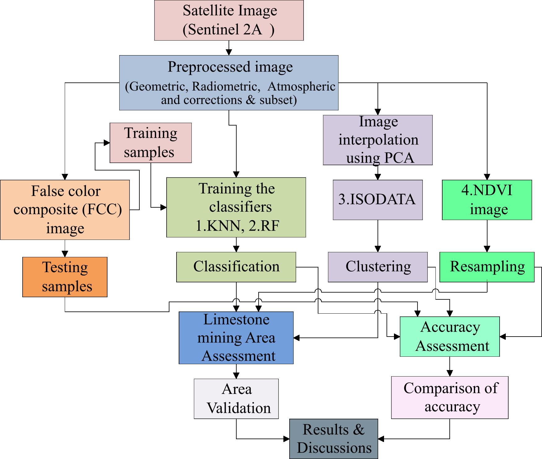

The study is conducted at the Yerraguntla cement industrial region, YSR Kadapa district, Andhra Pradesh, India as depicted in Fig. 1[14]. The study area has four cement industries and its captive limestone mines and Kadapa black stone slab mines in and around the Yerraguntla that was topographically lying 47 km west of YSR Kadapa district headquarters in the Rayalaseema region, Andhra Pradesh, India with Geographical Coordinates latitude 14.63 ${}^{\circ}$ N, longitude 78.53 ${}^{\circ}$ E, and average elevation 164 m [15]. Major cement industries and their captive limestone mining areas are portrayed with polygons shape files in Fig. 1. The summer (March–May) temperature of the area reaches 48 ${}^{\circ}$ C, while in the winter (December–February), it hovers at 14–27 ${}^{\circ}$ C.

3.2 Image processing

Table 1
Sentinel-2A bands and its applications

Sentinel-2 bands	Central wavelength ( $\mu$ m)	Spatial resolution (m)	Purpose in Level-2A processing context
B1 – Costal aerosol	0.443	60	Atmospheric Correction
B2 – Blue	0.490	10	Vegetation senescing, browning, and soil background; (aerosol scattering)
B3 – Green	0.560	10	Green peak, sensitive to total chlorophyll in vegetation
B4 – Red	0.665	10	Max Chlorophyll absorption
B5 – Vegetation red edge	0.705	20	Red edge position; consolidation of atmospheric corrections
B6 – Vegetation red edge	0.740	20	Red edge position; atmospheric correction; retrieval of aerosol load
B7 – Vegetation red edge	0.783	20	LAI; edge of the NIR plateau
B8 – Near infrared	0.842	10	Leaf Area Index (LAI)
B8a – Narrow near infrared	0.865	20	Used for water vapor absorption reference
B9 – Water vapor	0.945	60	Water vapor absorption, atmospheric correction
B10 – Shortwave infrared	1.375	60	Detection of thin cirrus for atmospheric correction
B11 – Shortwave infrared	1.610	20	Soils detection, Sensitive to lignin, starch, and forest above-ground biomass
B12 – Shortwave infrared	2.190	20	Assessment of vegetation conditions; monitoring of soil erosion

Classifier’s performance evaluation in the active Limestone mines mapping and area assessment was divided into three phases, the first phase included downloading, preprocessing, and clipping of the sentinel-2A imagery to the study area. The second phase includes spectral index (NDVI) calculation, training sample collection and training of the supervised machine learning model (KNN, RF), and dimensionality reduction using PCA for unsupervised learning (ISODATA). The third phase corresponds to the classification of the study area and mining area mapping. The fourth phase included classifier accuracy assessment followed by area calculation and validation. Figure 2 presents the workflow employed in the research.

3.2.1 Dataset collection

In the present research, we used the open-access USGS-NASA EarthEexplorer (https://earthexplorer.usgs.gov/) to download the Sentinel-2A (Level-2A product) dataset for March 25, 2019. Sentinel-2A contains 13 spectral bands (4 bands at 10 m, 6 bands at 20 m, and 3 bands at 60 m spatial resolution), as shown in Table 1, with central wavelengths ranging from 0.443 $\mu$ m to 2.190 $\mu$ m [16]. The Level-2A dataset processing includes Atmospheric Correction applied to Top-Of-Atmosphere (TOA) orthorectification or further processing.

3.2.2 Pre-processing

Figure 3.

Preprocessed true color Sentinel-2A image.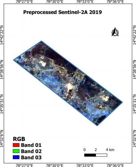

To get the data ready for further processing and analysis 10 m and 20 m spatial resolution bands of Sentinel-2A (60 m resolution bands were not utilized for this study) were geo-referenced to coordinate reference system EPSG:32644-WGS84/UTM Zone 44N followed by an atmospheric correction, pixel value conversion from digital number to mirror reflection, resampling, creating layer stack of nine bands and clipping to the area of interest (AOI) using the Semi-Automatic Classification Plugin (SCP) in QGIS tool [17]. Figure 3 shows a preprocessed Sentinel-2A image, with white representing the limestone mines, blue representing barren lands, and dark brown representing the following lands.

3.2.3 Training and testing samples collection

Figure 4.

False-color composite (FCC) of Sentinel-2A image.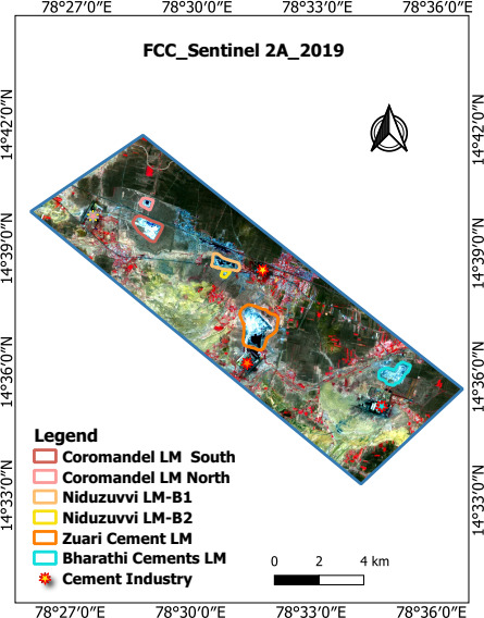

To map the active limestone mining area, the selection of the ground control points (GCPs) was performed based on Sentinel-2A images False Color Composite (FCC) created using band combination 7-3-2 [18] shown in Fig. 4. A total of 140 points (1, 28,795 pixels) were randomly selected over the study area having a minimum of 20 points for each class. The points were divided into 6 classes (water body, Limestone mine, Barren land, Follow land Built-up, and vegetation) using the visual interpretation in the FCC Sentinel-2A image. The red color shows the vegetation region, the white color region shows the limestone mining area, the yellow color region shows barren land, the dark brown region shows Follow land and the red mixed white region shows the built-up. The points were distributed as follows: 80% for training and 20% for testing. The training points were used to train the model and then the classification model was applied to the preprocessed Sentinel-2A image. The accuracy of the classification over the Sentinel-2A image was performed by generating an error matrix utilizing, the testing points. However, the effectiveness of many supervised classifiers varies with the training set size and application domain.

3.3 Spectral index method

3.3.1 NDVI threshold method

The NDVI has been one of the most extensively utilized vegetation indices in remote sensing since its inception in the 1970s. With the expanding availability of remotely sensed imagery, many people are using NDVI for applications of other than science. The NDVI is an efficient spectral index to locate vegetation cover, land cover (LC) changes caused by human activities, and water bodies [18]. The NDVI values are between $-$ 1 and $+$ 1 [19]. The Red and NIR bands of Sentinel-2A imagery are used to calculate NDVI, as illustrated in Eq. (1).

$\displaystyle\textit{NDVI}=\frac{\textit{NIR}-\textit{Red}}{\textit{NIR}+% \textit{Red}}$ (1)

Figure 5 shows the NDVI map in the Limestone mining sites dated March 25, 2019, where water bodies are indicated by negative NDVI values ( $-$ 1 to $-$ 0.16). Near-zero values ( $-$ 0.16 to 0.07) relate to limestone rocks. NDVI values from 0.07 to 0.29 correspond to bare soil surfaces plus barren lands, Low NDVI levels (0.29 to 0.51) are agricultural fields, but high NDVI values are prevalent for the dense vegetation (between 0.51 and 1.0) [20].

Table 2

NDVI threshold values for Land use/cover classes

Class	NDVI threshold values		Land use/cover class
	Minimum	Maximum
1.	$-$ 1.0	$-$ 0.1	Water bodies
2.	$-$ 0.1	0.05	Limestone mines
3.	0.05	0.15	Barren land
4.	0.15	0.2	Follow land
5.	0.2	0.3	Built-up
6.	0.3	1	Vegetation

Figure 5.

NDVI map of sentinel-2A for the study area.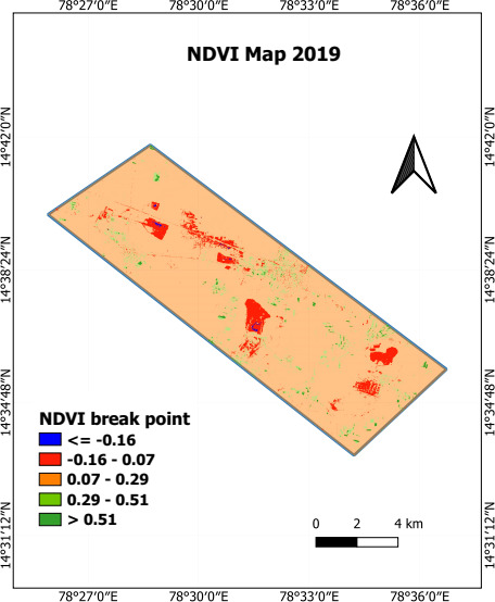

NDVI algorithm for classification

The algorithm is the hierarchy for a novel adaptive methodology for demarcating and assessing limestone mining areas based on the NDVI threshold method [20].

(a)

Satellite images are preprocessed and a layer stack is generated for data visualization using the Semi-Automatic Classification Plugin (SCP).

(b)

The layer stack image is clipped to the study area utilizing the SCP ‘Clip multiple raster tool’ and the study area shapefile.

(c)

The Red and Near-Infrared (NIR) bands of Sentinel-2A satellite imagery are used to generate NDVI values using the QGIS ‘raster calculator’.

(d)

Using the ‘reclassify by table’ processing tool and the Nearest-Neighbor method, the NDVI image is classified (resampled) into six land use/cover classes with the help of NDVI threshold values shown in Table 2.

(e)

The active mine area is determined using the ‘r.report’ processing tool.

(f)

The accuracy analysis feature of the SCP ‘post-processing tool’ was utilized to detect mapping errors.

(g)

The results obtained are compared to industrial report data.

3.4 Machine learning methods

For mineral mapping and lithological discrimination, the synergy of machine learning models and remote sensing data could be considered an efficient and economical solution. These methods are effectively data-driven methodologies and could be used to convert high-dimensional data into lower dimensions, forecast specific trends in the data, and identify particular traits in the data, among other things [21].

Table 3
Eigenvector from principal component analysis

	PC 1	PC 2	PC 3
Bandset 1	0.145	0.141	$-$ 0.433
Bandset 2	0.193	0.143	$-$ 0.456
Bandset 3	0.244	$-$ 0.023	$-$ 0.498
Information (%)	58.2	26.1	$-$ 13.86

Table 4

Selected ISODATA algorithm process parameters

Input parameter	Value/selection
Number of initial clusters ( $N$ )	10
Number of final clusters ( $N$ )	06
Threshold	0.01
Minimum number of iterations	10
Standard deviation	0.2
Minimum class size pixels	10
Distance algorithm	Minimum distance
Seed signatures	Random seed signatures

Figure 6.

PCA stacked image of Sentinel-2A.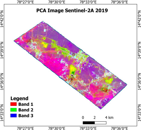

Machine learning models are classified into dimensionality reduction methods (e.g. Independent Component Analysis, Minimum Noise Fraction, and Principal Component Analysis(PCA)), Classification methods (e.g. Minimum distance, Support Vector Machines, Random Forest, simple Neural Networks), Clustering methods (e.g. K-means, ISODATA), Regression methods (e.g. Multi-Linear Regression, Multivariate Regression, Logistic Regression ), and deep learning methods (Convolutional Neural Network) [21, 22]. No algorithm is superior to another. The effectiveness of the algorithm is governed by the features of the landscape, training data, a complete comprehension of the classifier operations, and the user’s ability. There are several indices for evaluating an algorithm’s quality, including overall accuracy (OA), producer’s (PA), user’s (UA) accuracy, and kappa coefficient, These indicators values are greater the classification results are more accurate [23].

3.4.1 PCA – ISODATA classifier

There are several Supervised and unsupervised learning methods to interpret remotely-sensed images. Ground truth data are initially required for supervised image classification. When there is no ground truth data, unsupervised (clustering) algorithms such as ISODATA and K-Means can be preferable and plausible.

Principal Component Analysis (PCA) in conjunction with ISODATA clustering is a powerful method for visualizing high-dimensional datasets. PCA is a multivariate statistical technique frequently used in image processing to reduce data dimension or data decorrelation. In the present study, data is reduced to three principal components (PCs), and redundancy between highly correlated bands is reduced. We computed the Covariance matrix, Correlation matrix, and eigenvectors using SCP in QGIS and then applied the ISODATA clustering method to the layer-stacked PCA image. Figure 6 shows the layer-stacked PCA bands image and Table 3 illustrates the eigenvectors of the PCA.

The ISODATA algorithm is an amendment of the k-means clustering. To avoid misclassification, the analyst (user) must normally set parameters such as the minimum and maximum size of the cluster, the minimum separation between clusters, the minimum and the maximum number of clusters, and the maximum number of iterations [20]. Figure 7 depicts the PCA – ISODATA classifier workflow, while Table 4 depicts the process parameter selection.

Figure 7.

PCA – ISODATA classifier work flow.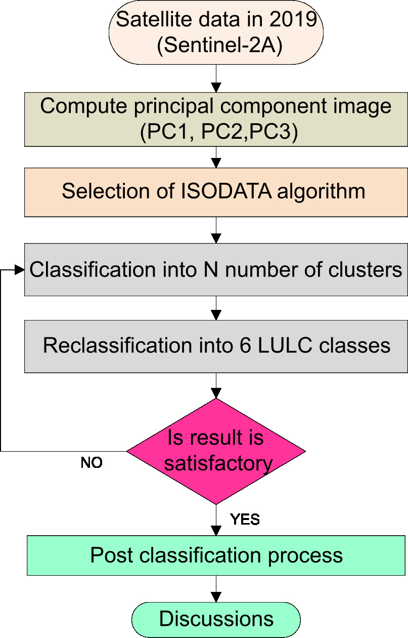

ISODATA algorithm for classification

(a)

Set the total number of spectral classes that will be grouped.

(b)

Choose an optimal number of cluster centres at random.

(c)

Assign each pixel to the nearest cluster based on the closest mean spectral Euclidean distance measure to the center mathematically expressed in Eq. (3).

(d)

For each cluster, calculate the Sum of Squared Error (SSE) between cluster centers using Eq. (2).

$\displaystyle\textit{SSE}=\sum_{j=1}^{k}\sum_{i=1}^{n}[D(i,j)-m_{j}]^{2}$ (2)

where $n=$ number of pixels enclosed in a given cluster. $D(i,j)=$ value of the $i^{\text{th}}$ pixel in the $j^{\text{th}}$ cluster $m_{j}=$ mean of the $j^{\text{th}}$ cluster

(i)

Adjust the center of each cluster if SSE is high and update it until the SSE reaches the specified minimum value.

(ii)

Split the clusters if it contains a large number of pixels exceeding the predetermined threshold.

(iii)

Merge the clusters if the distance between the clusters is less than the predetermined threshold.

(e)

Repeat the iterations with new cluster centers.

(f)

Continue iterations until:

(i)

The average inter-center distance is less than the user-specified threshold.

(ii)

If the average changes in inter-center distance between iterations are less than a specific threshold.

(iii)

The maximum number of iterations has been reached.

(g)

Image classification results for post-classification analysis.

3.4.2 K-Nearest Neighbors (KNN) classification

Figure 8.

KNN Classifier work flow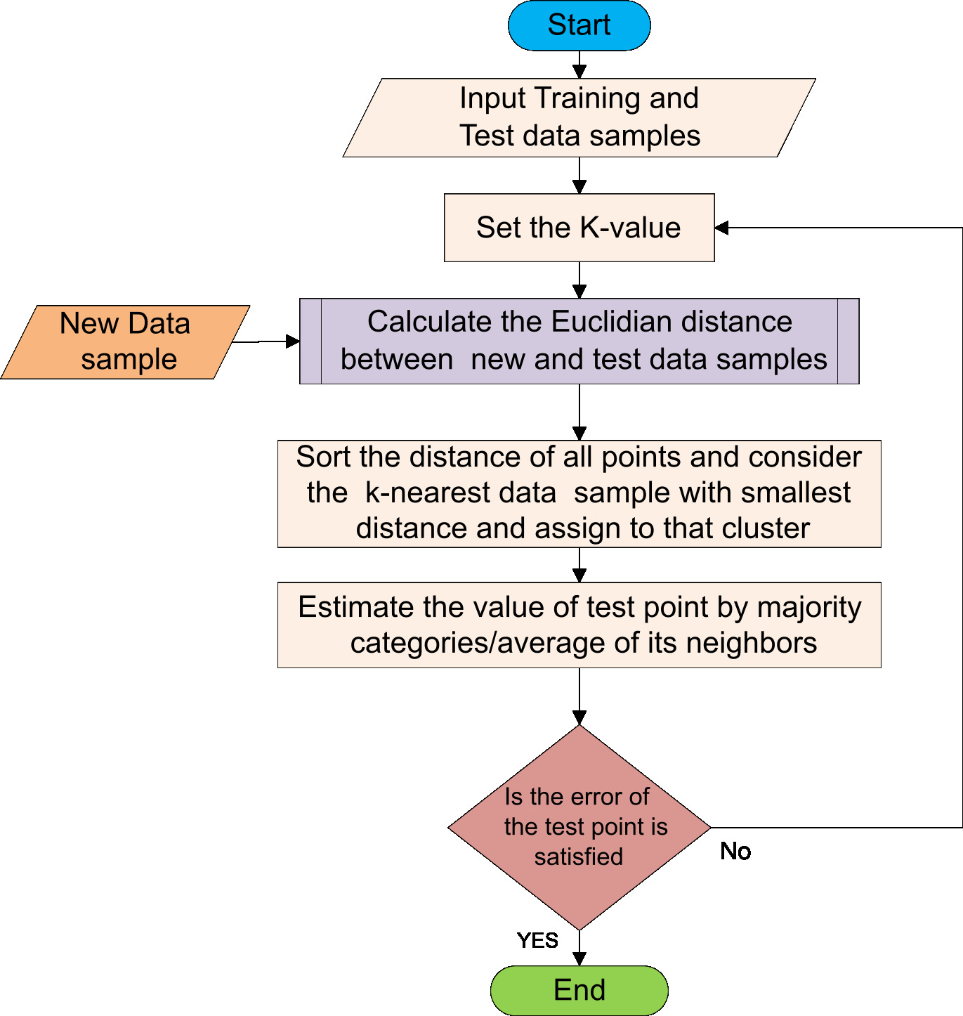

The KNN is a supervised machine learning classifier that is nonparametric memory-based. After determining the number of neighbors, the algorithm will classify the pixels based on the sample values of the ( $K=$ 10) nearest neighbors. This approach is highly fast when $K$ is low, but it is a sluggish method when there are numerous samples and $K$ is high. KNN classification is applied to the study area using QGIS’s “dzetsaka classification plugin” and Scikit-Learn Library [22]. The KNN classifier work flow is illustrated in Fig. 8 and and selected process parameter listed in Table 5.

KNN algorithm for classification

(a)

Data preprocessing.

(b)

Fitting the K-NN classifier to the Training data (Training the model).

(c)

Select the number $K$ of the neighbors.

(d)

Consider all points and the new points in an $n$ -dimensional space.

(e)

Calculate the Euclidean distance of new points from all points using Eq. (3).

$\displaystyle D(m_{ik})=\sqrt{\sum_{j=1}^{\textit{nb}}(m_{ij}-k_{j})^{2}}$ (3)

Where

–

nb $=$ number of bands

–

$j=$ particular band

–

$i=$ particular band

–

$k_{j}=$ digital number (DN) value of a pixel $k$ in band $j$

–

$m_{ij}=$ mean DN value of pixels in band $j$ for the sample class $i$

–

$D(m_{ik})=$ Euclidean distance from the mean of a class to any unknown pixel

(f)

Sort the distance of all points and select the $K$ nearest neighbor’s points with the smallest distance (neighbor).

(g)

Count how many data points there are in each group among these $K$ -nearest neighbors.

(h)

Allocate the new data points to the group that has the most neighbors.

(i)

If the error of the test points is satisfactory, terminate the process; otherwise, repeat steps (c) to (h).

3.4.3 Random forest (RF) classifier

Table 5
Selected RF algorithm process parameters

Input parameter	Value/selection
Ground control points (GCPs)	140 points (1, 28,795 pixels)
Training data ( $N$ )	80% of GCPs
Testing data	20% of GCPs
Instances ( $n$ )	3000
Features ( $p$ )	36
Number of classifiers ( $B$ )	10
Iterations ( $K$ )	6

Figure 9.

Hierarchy diagram of Random forest algorithm.

The RF classifier is an ensemble method using decision trees as classifiers [24]. It works on the feature aggregating (bagging) a huge number of decision trees using the bootstrap of the sample from training data. The decision of majority of the trees is chosen as the final output [25, 26, 27]. In this study, RF classification was applied to the Sentinel-2A image using QGIS’s “dzetsaka classification plugin” [22, 27, 28]. The Hierarchy structure of the RF algorithm is depicted in Fig. 9 in that the Root-Branch-Leaf node makes the decision trees. The decision tree’s root node reflects the most appropriate image feature. The branch nodes separate the data into groups with diverse rules. The image data categorization results are obtained via the leaf nodes. The classification error for each tree is estimated from out-of-bag (OOB) data. The RF algorithm process parameter listed in Table 5.

Figure 10.

ISODATA and NDVI classification.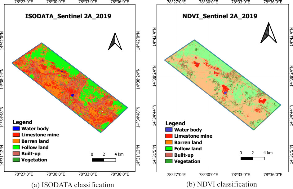

Figure 11.

KNN and RF supervised classification.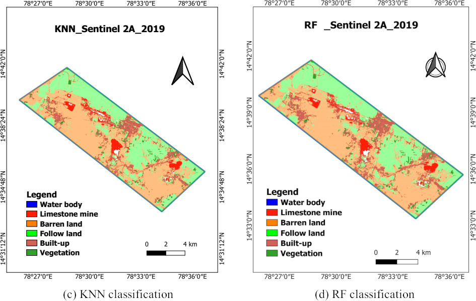

Random forest algorithm for classification

Training Phase:

Considerations:

$N$ : Training data set with $n$ -instances, $p$ features, and the target variable

$K$ : Number of classes in the target variable

$B$ : Number of classifiers in RF

Procedure:

For sample $b=$ 1 to $B$

Take a bootstrapped sample $D_{b}^{*}$ from the training data set $N$ .

Develop a tree using a random feature subset from the bootstrapped sample $D_{b}^{*}$ .

For a given node $t$ ,

(i).

Choose sample $m=\sqrt{p}$ features at random from the $p$ variables.

(ii).

Compute the best-spilt features and cut points using the random feature subset.

(iii).

Split down the data using the finest split features and cut points. Repeat steps (i) to (iii) until the minimum node size $n_{\text{min}}$ is reached

Create trained classifiers $C_{b}$ .

Test Phase:

Using a simple majority vote, aggregate the B-Trained classifiers. The predicted class label from classifiers $C_{B}$ for a test case, $x$ is:

$\displaystyle C_{B}(x)=\textit{argmax}_{j}\sum_{b=1}^{B}I(C_{b}(x)=j),\quad% \text{for}\ j=1,2,\ldots,K$

4. Results and discussions

Table 6
Confusion matrix for the NDVI classifier

		$>$ Ground truth data (reference pixels)
	Land class	Water body	Limestone mine	Barren land	Follow land	Build-up	Vegetation	User’s sum	UA (%)
$>$ Classified	Waterbody	1120	1	0	0	0	0	1121	99.91
class data	Limestone mine	140	6683	55	0	0	260	7138	93.63
	Barren land	2	451	56414	4000	0	3221	64088	88.02
	Follow land	0	0	3790	45632	5	1449	50876	89.69
	Build-up	0	0	254	622	199	2674	3749	5.31
	Vegetation	0	0	0	1	1593	229	1823	12.56
	Producer’s sum	1262	7135	60513	50255	1797	7833	128795 ( $N$ )
	PA (%)	74.67	92.04	92.65	87.79	22.42	2.323
	Overall accuracy (%) $=$ 79.84
	Kappa hat $=$ 0.685

Table 7

Confusion matrix for the ISODATA classifier

		$>$ Ground truth data (reference pixels)
	Land class	Water body	Limestone mine	Barren land	Follow land	Build-up	Vegetation	User’s sum	UA (%)
$>$ Classified	Waterbody	1024	0	0	0	0	0	1024	100.00
class data	Limestone mine	18	5422	14443	8	5	2917	22813	23.77
	Barren land	41	426	36704	8071	5	474	45721	80.28
	Follow land	0	0	1212	41815	7	11	43045	97.14
	Build-up	0	0	0	0	1567	92	1659	94.45
	Vegetation	0	1287	8154	361	213	4339	14354	30.23
	Producer’s sum	1083	7135	60513	50255	1797	7833	128616 ( $N$ )
	PA (%)	84.24	65.83	53.31	78.91	81.24	69.99
	Overall accuracy (%) $=$ 64.16
	Kappa hat $=$ 0.4990

Table 8

Confusion matrix for the KNN classifier

		$>$ Ground truth data (reference pixels)
	Land class	Water body	Limestone mine	Barren land	Follow land	Build-up	Vegetation	User’s sum	UA (%)
$>$ Classified	Waterbody	1148	58	55	0	0	0	1261	100.00
class data	Limestone mine	59	7071	1	0	0	12	7143	98.99
	Barren land	25	0	58053	2119	210	120	60527	95.91
	Follow land	30	0	1845	47623	0	755	50253	94.76
	Build-up	0	0	519	0	1258	13	1790	70.27
	Vegetation	0	6	40	513	329	6933	7821	88.64
	Producer’s sum	1262	7135	60513	50255	1797	7833	128795 ( $N$ )
	PA (%)	90.96	99.10	95.94	94.76	70.00	88.51
	Overall accuracy (%) $=$ 94.78
	Kappa hat $=$ 0.947

Table 9

Confusion matrix for the RF classifier

		$>$ Ground truth data (reference pixels)
	Land class	Water body	Limestone mine	Barren land	Follow land	Build-up	Vegetation	User’s sum	UA (%)
$>$ Classified	Waterbody	1193	32	0	31	0	0	1256	97.38
class data	Limestone mine	63	7077	14	0	0	123	7277	97.25
	Barren land	6	12	59053	1129	31	499	60730	97.23
	Follow land	0	0	1359	48251	6	596	50212	96.09
	Build-up	0	0	0	52	1475	288	1815	81.12
	Vegetation	0	14	87	792	285	6327	7505	84.30
	Producer’s sum	1262	7135	60513	50255	1797	7833	128795 ( $N$ )
	PA (%)	94.53	99.18	97.58	96.01	82.08	80.77
	Overall accuracy (%) $=$ 95.79
	Kappa hat $=$ 0.957

While identifying the limestone mines in the Yerraguntla cement industrial region, ISODATA was not able to identify the expected clusters. It can be concluded that the ISODATA clustering technique is not able to identify correct and one-label clusters. Due to similar spectral reflectance of land cover types (built-up and Limestone mines), two or more classes can be mixed and some clusters cannot be linked to the land cover (Fig. 10). Figure 11 shows the limestone mining area including barren lands, follow lands, built-up, and vegetation land cover classes’ mapped using supervised machine learning algorithms KNN and RF.

4.1 Performance evaluation

The major performance metrics for validating machine learning methods include the confusion matrix, AUC-ROC Curve, precision, accuracy, F1-score, recall, Log Loss, or Cross Entropy. The use of a confusion matrix to assess accuracy has become standard practice in the quality assessment of remote sensing products. Hence we used the confusion matrix to evaluate the accuracy of classifiers in this article [25]. The confusion matrix is a table that compares the categorized pixels (model predictions) to the Ground-Truth points (validation pixels). The rows of the confusion matrix represent an instance in a classified class, while columns represent an instance in the ground truth data. The diagonal elements show the accurately classified image pixels for each class.

In this study, we used the SCP post-processing tool in QGIS software to compute the confusion matrix, which we then used in Microsoft Excel to calculate statistical metrics such as Users Accuracy (UA), Producer’s Accuracy (PA), Overall Accuracy, and Kappa coefficient (K) [20] using the Eqs (4)–(7).

$\displaystyle\text{producer's accuracy of a class}\ =\frac{\textit{Number of % correctly classified pixels of a class}}{\textit{Sum pruducer in a column}}$ (4) $\displaystyle\text{user's accuracy of a class}\ =\frac{\textit{Number of % correctly classified pixels of a class}}{\textit{Sum user in a column}}$ (5) $\displaystyle\text{overall accuracy}\ =\frac{\textit{Sum correctly classified % pixels}}{\textit{Sum of pixels used for accuracy assessment}\ (N)}$ (6) $\displaystyle\text{kappa hat}\ =\frac{N\sum_{i=1}^{r}X_{ii}-\sum_{i=1}^{r}(X_{% i+}*X_{+j})}{N^{2}-\sum_{i=1}^{r}(X_{i+}*X_{+j})}$ (7)

where $r$ is the number of rows in the error matrix, $X_{ii}$ is the number of observed pixels in row $i$ and column $i$ , $X_{i+}$ and $X_{+j}$ are the land class totals for row $i$ and column $j$ , respectively, and $N$ is the total number of pixels used for accuracy assessment.

Tables 6–9 show the highest and lowest accuracy of classifiers for six different land classes. The Random Forest classifier outperformed the other classifiers in terms of accuracy because it is the best possible method for handling missing data and can handle large datasets with high dimensionality. It prevents overfitting issues.

4.2 Accuracy assessment

Table 10
LULC kappa coefficient and overall accuracy (OA) with Sentinel-2A image

S. No.	Methods	Kappa hat	A degree of agreement	Overall accuracy (%)
1	NDVI	0.685	substantial	79.84
2	ISODATA	0.499	moderate	64.16
3	KNN	0.947	Perfect	94.78
4	RF	0.957	Perfect	95.79

Table 11

Producer, User accuracy, and area of limestone mines with Sentinel-2A image

S. No	Classification method	UA accuracy (%)	PA accuracy (%)	Limestone mine area (Hectares)
1.	NDVI	93.63	92.04	469.92
2.	ISODATA	23.77	65.83	2003.65
3.	KNN	98.99	99.10	417.47
4.	RF	97.25	99.18	379.57
5.	Industrial data	–	–	487.10

Figure 12.

Classification of overall accuracy using different algorithms.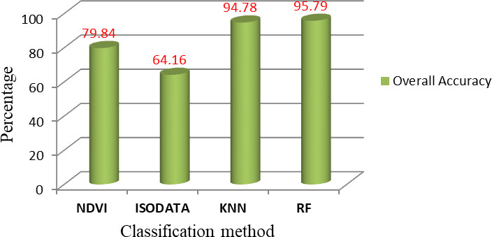

Figure 13.

Active Mine area validation with industrial data.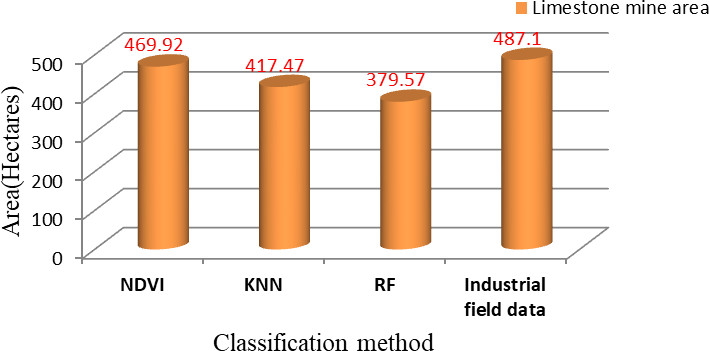

The mapped active limestone mine areas, as well as the comparison of overall accuracy and kappa coefficient for land use/cover (LULC) class to the four classifiers, are illustrated in Table 10 and Fig. 12. The accuracy assessment for the Limestone mine class was performed using an independent validation dataset, as shown in Table 10. The kappa coefficient ranges from 0 to 1, where 1 signifies perfect agreement and 0 signifies no agreement [29].

4.3 Mining area validation

The classification algorithms estimated limestone mine area is compared with industrial field data illustrated in Fig. 13 and Table 11. According to the mapping results, in 2019 we observed an active mining area is 469.92 ha from the NDVI-classified Sentinel-2A image and 417.47 ha from KNN, and 379.57 ha from the RF classifier. These are compared with the original active mining area of industry (487.1 ha). The deviation in the area is due to the classified methods showing mine pit water bodies (of area 27.69 ha) as a separate class from the mining area. In this study, the area was computed using ‘r.report’ in the processing toolbox of the QGIS 3.18.

5. Conclusions

In this research paper, we explored the performance of the spectral index, unsupervised and supervised machine learning algorithms in the determination of limestone mine area and land use/cover classes. The Random Forest technique achieved the best results in terms of getting more accurate LULC maps, with an overall accuracy of 95.79% and a kappa coefficient of 0.957, although the limestone mine area was low (379.57 ha) compared to the industrial data area of 487.10 ha. With an overall accuracy of 94.78%, a kappa coefficient of 0.947, and a mine area of 417.47 ha, the KNN approach placed second. Following that, the spectral index (NDVI) method placed in the third category, with an overall accuracy of 79.84% and an estimated limestone mine area of 469.92 ha, which is extremely near to industrial field data. The lowest accuracy is occupied by the ISODATA method that’s 64.16%. When running the KNN and RF algorithms in QGIS using the “dzetsaka classification tool”, the default parameters were utilized. Improved results might be obtained by deep learning algorithms. This study gives a model for environmental impact assessment in industrial areas for limestone mine owners and environmental engineers with mining area mapping and monitoring.

Footnotes

Acknowledgments

The author is grateful to the management of the Limestone Mine and Cement Industries for allowing him to conduct fieldwork in the study area.

Funding

The authors also declare that there is no source of funding for this work.

References

Indian Bureau of Mines. Indian Minerals Yearbook 2020 (Part-III: Mineral Reviews). Nagpur 13, Government of India Ministry of Mines: 2021. pp. 18.1-18.21.

Sudhakar

Reddy

. Land use/land cover change assessment of Ysr Kadapa District, Andhra Pradesh, India using IRS resourcesat-1/2 LISS III multi-temporal open source data. International Journal of Recent Technology and Engineering. 2019; 3(4): 20. doi: 10.35940/ijrte.C6067.098319.

Wang

Niu

. Eco-environmental assessment model of the mining area in Gongyi, China. Scientific Reports. 2021 Sep 2; 11(1): 17549. doi: 10.1038/s41598-021-96625-9.

Shirmard

Farahbakhsh

Müller

Chandra

. A review of machine learning in processing remote sensing data for mineral exploration. Remote Sensing of Environment. 2022 Jan 1; 268: 112750. doi: 10.1016/j.rse.2021.112750.

Zerrouki

Harrou

Sun

Hocini

. A machine learning-based approach for land cover change detection using remote sensing and radiometric measurements. IEEE Sensors Journal. 2019 Mar 10; 19(14): 5843-50. doi: 10.1109/jsen.2019.2904137.

Roscher

Bohn

Duarte

Garcke

. Explain it to me–facing remote sensing challenges in the bio-and geosciences with explainable machine learning. ISPRS Annals of the Photogrammetry, Remote Sensing and Spatial Information Sciences. 2020 Aug 3; 3: 817-24. doi: 10.5194/isprs-annals-V-3-2020-817-2020.

Wang

Zuo

Dong

. Mapping of himalaya leucogranites based on ASTER and sentinel-2A datasets using a hybrid method of metric learning and random forest. IEEE Journal of Selected Topics in Applied Earth Observations and Remote Sensing. 2020 Apr 27; 13: 1925-36.

Wang

Zuo

Jing

. Fusion of geochemical and remote-sensing data for lithological mapping using random forest metric learning. Mathematical Geosciences. 2021 Aug; 53: 1125-45. doi: 10.1007/s11004-020-09897-8.

Bachri

Hakdaoui

Raji

Benbouziane

. Geological mapping using random forests applied to remote sensing data: a demonstration study from Msaidira-Souk Al Had, Sidi Ifni inlier (Western Anti-Atlas, Morocco). In: 2020 IEEE International conference of Moroccan Geomatics (Morgeo). IEEE; 2020 May 11. pp. 1-5. doi: 10.1109/Morgeo49228.2020.9121888.

10.

Abdolmaleki

Rasmussen

Pal

. Exploration of IOCG mineralizations using integration of space-borne remote sensing data with airborne geophysical data. The International Archives of the Photogrammetry, Remote Sensing and Spatial Information Sciences. 2020 Aug 21; 43: 9-16. doi: 10.5194/isprs-archives-XLIII-B3-2020-9-2020.

11.

Davids

Rouyet

. Remote sensing for the mining industry. Report, Project RESEM. 2018. ISBN: 978-82-7492-417-8.

12.

El Atillah

El Morjani

Souhassou

. Use of the sentinel-2A multispectral image for litho-structural and alteration mapping in Al Glo’a map sheet (1/50,000)(Bou Azzer–El Graara Inlier, Central Anti-Atlas, Morocco). Artificial Satellites. 2019 Sep; 54(3): 73-96. doi: 10.2478/arsa-2019-0007.

13.

Rahman

Abdullah

Tanzir

Hossain

Khan

Miah

Islam

. Performance of different machine learning algorithms on satellite image classification in rural and urban setup. Remote Sensing Applications: Society and Environment. 2020 Nov 1; 20: 100410. doi: 10.1016/j.rsase.2020.100410.

14.

Sudhakar

Reddy

. Land use Land cover change Assessment at Cement Industrial area using Landsat data-hybrid classification in part of YSR Kadapa District, Andhra Pradesh, India. International Journal of Intelligent Systems and Applications in Engineering. 2022 Mar 30; 10(1): 75-86. doi: 10.18201/ijisae.2022.270.

15.

Venkata Sudhakar

Reddy

Rani

. Delineation of the Captive Limestone Mine Boundaries Using Multispectral Satellite Images Through the Use of NDVI and Google Earth Image Template Matching. In: Proceedings of the International Conference on Innovative Computing & Communication (ICICC). 2022 Apr 23. doi: 10.2139/ssrn.4091402.

16.

Main-Knorn

Pflug

Louis

Debaecker

Müller-Wilm

Gascon

. Sen2Cor for Sentinel-2. In: Proc. SPIE 10427, Image and Signal Processing for Remote Sensing XXIII. 2017. p. 1042704. doi: 10.1117/12.2278218.

17.

Deliry

Avdan

. Extracting urban impervious surfaces from Sentinel-2 and Landsat-8 satellite data for urban planning and environmental management. Environmental Science and Pollution Research. 2021 Feb; 28(6): 6572-86. doi: 10.1007/s11356-020-11007-4.

18.

Somvanshi

Kumari

. Comparative analysis of different vegetation indices with respect to atmospheric particulate pollution using sentinel data. Applied Computing and Geosciences. 2020 Sep 1; 7: 100032. doi: 10.1016/j.acags.2020.100032.

19.

Kotaridis

Lazaridou

. Delineation of Open-Pit Mining Boundaries on Multispectral Imagery. In: Remote Sensing. IntechOpen; 2020 Oct 14. p. 10. doi: 10.5772/intechopen.94120.

20.

Sudhakar

Reddy

Rani

. Delineation and evaluation of the captive limestone mining area change and its influence on the environment using multispectral satellite images for industrial long-term sustainability. Cleaner Engineering and Technology. 2022 Oct 1; 10: 100551. doi: 10.1016/j.clet.2022.100551.

21.

Shirmard

Farahbakhsh

Beiranvand Pour

Muslim

Müller

Chandra

. Integration of selective dimensionality reduction techniques for mineral exploration using ASTER satellite data. Remote Sensing. 2020 Apr 16; 12(8): 1261. doi: 10.3390/rs12081261.

22.

Karasiak

Perbet

. Remote sensing of distinctive vegetation in Guiana amazonian park. In: QGIS and Applications in Agriculture and Forest, vol. 2. 2018 Jan 13. pp. 215-45. doi: 10.1002/9781119457107.ch7.

23.

Çığşar

Ünal

. Comparison of data mining classification algorithms determining the default risk. Scientific Programming. 2019 Feb 3; 2019. doi: 10.1155/2019/8706505.

24.

Hastie

Tibshirani

Friedman

. The elements of statistical learning: data mining, inference, and prediction. New York: Springer; 2009 Aug. doi: 10.1007/978-0-387-84858-7.

25.

Alshari

Gawali

. Analysis of machine learning techniques for sentinel-2A satellite images. Journal of Electrical and Computer Engineering. 2022 May 16; 2022: 1-6. doi: 10.1155/2022/9092299.

26.

Han

Kim

Lee

. Double random forest. Mach Learn. 2020; 109: 1569-1586. doi: 10.1007/s10994-020-05889-1.

27.

Maxwell

Warner

Fang

. Implementation of machine-learning classification in remote sensing: An applied review. International journal of remote sensing. 2018 May 3; 39(9): 2784-2817. doi: 10.1080/01431161.2018.1433343.

28.

Song

Liu

. Multi-label spacecraft electrical signal classification method based on DBN and random forest. PLoS One. 2017 May 9; 12(5): e0176614. doi: 10.1371/journal.pone.0176614.

29.

Landis

Koch

. The measurement of observer agreement for categorical data. Biometrics. 1977; 33(1): 159174. doi: 10.2307/2529310.

Assessment of open-pit captive limestone mining areas using sentinel-2 imagery with spectral indices and machine learning algorithms

Abstract

Keywords

1. Introduction

2. Literature review

3. Materials and methods

3.1 Study area

Table 1 Sentinel-2A bands and its applications

3.2.2 Pre-processing

3.3.1 NDVI threshold method

Table 3 Eigenvector from principal component analysis

Table 5 Selected RF algorithm process parameters

Table 6 Confusion matrix for the NDVI classifier

Table 10 LULC kappa coefficient and overall accuracy (OA) with Sentinel-2A image

5. Conclusions

Footnotes

Acknowledgments

Funding

References

Table 1
Sentinel-2A bands and its applications

Table 3
Eigenvector from principal component analysis

Table 5
Selected RF algorithm process parameters

Table 6
Confusion matrix for the NDVI classifier

Table 10
LULC kappa coefficient and overall accuracy (OA) with Sentinel-2A image