Construction of trail networks based on growing self-organizing maps and public GPS data

Abstract

Manual creation of trail maps for hikers is time-consuming and can be inaccurate. This paper presents a new method to construct trail networks based on a growing self-organizing map (GSOM) using publicly available Global Positioning System (GPS) data. Unlike other network topology construction techniques, this approach is not dependent on sequential GPS traces. Fine-tuning multiple hyperparameters enables to customize this process based on unique features of datasets and networks. The generated maps, which are trained on public GPS data, are compared to a ground truth from Open Street Map (OSM). The performance evaluation is based on the accuracy, completeness, and topological correctness of the trail maps. The proposed approach outperforms, particularly on sparse networks without significant GPS noise.

Keywords

Global Positioning System (GPS) data trail map construction growing self-organizing maps

1. Introduction

Trail maps are topological networks that are essential for navigation [1]. Trails are made up of various path segments that may intersect at certain points. The ability to navigate these paths successfully is crucial for the safety and enjoyment of both recreational hikers and those involved in search and rescue efforts.

Trail maps are typically created by cartographers and surveyors with specialized equipment. Although these techniques generate acceptable results, they are costly and time-consuming [1].

With the emergence of cost-effective GPS recording devices such as smartphones, smart watches, etc., the development of trail maps leveraging such data has become viable.

With the rise of collaborative crowd-sourced mapping, OpenStreetMap (OSM) has emerged as a popular platform. It allows users to make edits to streets, sidewalks, trail paths, and other cartography features. However, public GPS traces uploaded by users are prone to irregularities and noise, which could affect the quality of the data. Additionally, OSM trace datasets suffer from limited geographic representation, the use of low-cost and low-quality devices, and individuals who have wandered off the established trails. Ideally, a set of user-uploaded traces would be from a heterogeneous set of GPS recording devices; however, this may not always be true, which may introduce bias.

Much work has been done using both OSM as a model for ground truth comparison as well as utilizing its public GPS data for training [2].

As GPS data often suffer from signal attenuation problems as pedestrians walk under tree cover or near buildings, algorithms using this data must be resistant to high noise traces.

This paper introduces a novel approach for trail network construction, which involves utilizing a growing self-organizing map (GSOM) and applying connection and contraction rules. This methodology is motivated by previous research that has utilized GSOMs to approximate principal curves as well as SOMs to generate road networks [3, 4]. As a method of unsupervised learning, self-organizing maps have seen recent use in identifying fault modes and diagnosis [5]. Self-organizing maps have also been embedded in a more extensive neural architecture to improve quantization and topology in latent space; these are called deep-embedded self-organizing maps [6].

[2] establishes a set of benchmark metrics for evaluating different network construction methods. These metrics include precision, completeness, and topological correctness. To evaluate their proposed method, the authors constructed networks using Kernel Density Estimation from OSM traces and reported the results of the metric evaluation. Additionally, a section of the paper will focus on comparing the performance of their approach with our proposed methods using the same dataset and benchmark metrics.

2. Background

2.1 Preliminaries

.

A trajectory $T$ of size $n$ is a sequence of spatial points $T:p_{1}\rightarrow p_{2}\rightarrow\ldots\rightarrow p_{n}$ that are sampled from an object that is continuously moving. Each point $p_{i}$ has a two-dimensional coordinate $p_{i}=(x_{i},y_{i})\in R_{2}$ and a timestamp $t_{i}$ . Points in $T$ are sorted based on their timestamps. Definition of a trajectory used from [7].

Many existing works utilize trajectory-based traces where GPS points are sequentially ordered [8, 1, 9, 7]. We can anonymize a trace by removing the sequential ordering of nodes. OSM anonymizes many of their public GPS traces, so we primarily utilize anonymized traces, which adds a layer of complexity to the linking step of our algorithm and a difference to many existing works. Figure 1 illustrates the process of anonymizing a GPS trajectory.

We have formally defined an anonymized trace in the following definition based on the data that is represented largely from OSM.

.

An anonymized trace $T$ of size $n$ is a set of spatial points $T={p_{1},p_{2},\ldots,p_{n}}$ sampled from a continuously in motion object. Each point $p_{i}$ has a two-dimensional coordinate $p_{i}=(x_{i},y_{i})\in R_{2}$ which has no timestamp.

Since our focus is the inclusion of hiking trails and due to the nature of our construction algorithm, we present slightly different definitions of networks or maps [7]. However, the underlying structure is the same.

.

A road or trail network or (map) is a graph $G=(V,E)$ , in which a vertex $v=(x,y)\in V$ denotes a point along a road or trail (or intersection point between trails/roads) and edges $e=(x,y)\in E$ represents two points $p_{1},p_{2}$ are connected by a trail/road.

Figure 1.

Trace anonymization.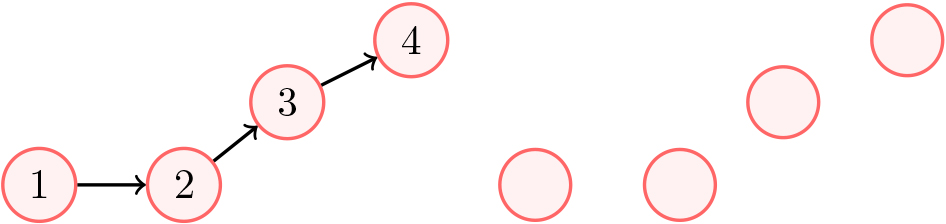

2.2 Method archetypes

Two primary sources of data, namely GPS data or aerial imagery, are used to infer roads and trails. Although algorithms using imagery can be efficient, they often suffer from inconsistent or low-quality data sources due to high costs. Moreover, physical features such as visual obstruction and variable weather conditions can also introduce errors into the system. The authors have covered these issues in their work [10, 11]. Certain types of neural networks are used to analyze this aerial imagery for analysis of human activities [12].

However, some algorithms use GPS data recorded by mobile phones or smart watches to make road network inferences. This approach provides access to a wide range of data; however, GPS errors can lead to inaccuracies in network inference. This paper primarily focuses on this data inference source.

There are four method archetypes available for constructing road and pedestrian path networks from GPS data sources: 1. Point clustering, 2. Kernel Density Estimation, 3. Trace merging, and 4. Intersection Linking [7].

2.2.1 Point clustering

The main purpose of a clustering algorithm is to create a representative collection of data points from the input dataset that accurately describes the fundamental geometry. In order to determine the positions of these representative nodes, K-means was utilized. However, in this paper, a GSOM approach was adopted, which is analogous to K-means. Usually, Vincenty distances (for longitude and latitude coordinates) or Euclidean are employed to measure the distance. Once the set of representative nodes is established, a linking step is carried out to create the topology of the network [9]. The techniques used for creating edges between nodes differ depending on the approach. An approach that leverages trajectory-based GPS traces, that are not anonymized, involves utilizing information from these traces to establish connections between the nodes. For instance, the angle of the heading contained within the GPS trajectories can be utilized to establish edges [13].

The algorithm outlined in this paper is a type of point clustering approach that incorporates a novel component to use anonymized traces.

[4] employs a GSOM to generate a map of roads based on satellite imagery. The nodes of the map are created by neurons that adapt to the varying colors of a road in contrast to its background, while the edges are created through pattern matching. The final step matches the structure of the map to the templates.

2.2.2 Kernel density estimation (KDE)

In KDE approaches, it is common practice to create a function of traces based on probability density as the first step. To visualize the data, an image is created based on pixel value of each intersection of traces. In the next step, outliers and errors are discarded by using a threshold. Then the outlines of road line are calculated using various methods, such as Voronoi diagrams. Once the road outlines are computed, intersections are extracted from them. This process finalized the generated road network [9].

In [14], a KDE approach using point clustering algorithm was proposed to create walking paths using filtered trajectories.

In a typical KDE algorithm, trajectory information is used to create a histogram that is used to produce the discretized image. Though it is possible to adapt many of these algorithms for anonymized traces, performance may vary.

2.2.3 Trace merging

Trace merging approaches are a unique type of algorithms that aggregate trajectories into a network that grows continuously. The process involves aading new traces to the network incrementally. If there is no overlap between the new trace and the network, the added trace will be completely included in the net work. If any overlap exists, the edges’ weights will be adjusted in those parts of the network. In this process, the constraints of the existing network should be met to ensure that the system is actively learning [9].

Most known examples are variations on this fundamental idea. [15] instead of presenting trajectories one at a time, creates clusters of sub-trajectories, which are then iteratively presented to the existing network.

As these approaches require explicit traces, they cannot be applied to anonymized traces.

2.2.4 Intersection linking

This technique first identify intersections and then link these crossings based on trace data [7]. In [8], to determine the intersections, the turning changes are utilized.

The process involves extracting points from input traces that correlates with changes in the turning (heading) or speed. Then the created data points are clustered to form one intersection point for each cluster, link these cluster intersection points using trace data that crosses multiple intersections.

This process relies heavily on the proper identification of intersections. It also requires information from a trajectory, such as heading and speed, and could not be used for anonymized traces.

2.2.5 GSOM method

Our Growing Self-Organizing algorithm has a structure that is analogous to many point clustering techniques, consisting of a two step approach to identify points, followed by a linking process. However, what sets our algorithm apart from many common methods is the utilization of anonymized trajectories. This approach allows us to use public GPS data to be used in the analysis.

3. Methodology

The main component of this approach is the utilization of a GSOM, which is a type of self-organizing map (SOM) that functions as a neural network. For a given dataset, a data point is fed into the SOM, and one neuron is selected as the winner. The GSOM then employs a weight adjustment that includes the winning node and some neighboring nodes based on a threshold distance.

The GSOM has the ability to expand its number of neurons dynamically. This means that when a new data point is fed to the GSOM and it is not adequately represented by the existing neurons, the algorithm can create new neurons to better capture the characteristics of the data.

This process involves five major steps: initialization, growth and learning, connection rule, collapsing, and smoothing.

Figure 2.

Methodology overview.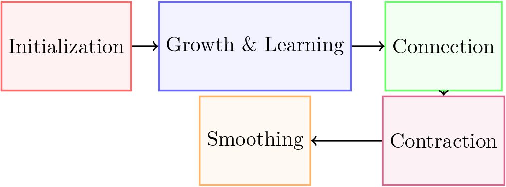

3.1 Initialization

To initialize the GSOM, the weights of three nodes are randomly selected from the points in the dataset.

The spread factor $S F$ and neighborhood radius $R$ as hyperparameters are initialized. A growth threshold $G T$ is calculated based on the spread factor.

$\displaystyle GT=-2*\ln{SF}$ (1)

The following algorithm is performed on the dataset to remove points that do not have sufficient density. This was commonly caused by a single off-trail trace.

: Clean Data[1] CleanDataD, runordered dataset D, r cleaning radius newDataInitialize empty list $p\in D$ flag $\leftarrow$ True $q\in D-\{p\}$ $d(p,q)<r$ d is distance (Eq. (2)) flag $\leftarrow$ False flag newData.append ( $p$ )Add $p$ to newData newData

3.2 Growth and learning

In this segment of the algorithm, the process involves learning, which includes adapting weights and generating new neurons. The network $N$ with neurons $n\in N$ is presented with one datapoint ( $p\in D$ dataset) at a time. Where the Euclidean distance between $p$ and $n$ is $d$ . $p_{1}$ represents the value of x, and $p_{2}$ , the value of y.

$\displaystyle d=p-n=\sqrt{(p_{1}-n_{1})^{2}+(p_{2}-n_{2})^{2}}$ (2)

Algorithm 3.2 describes the learning and growing phase in our approach. The terminal condition is reached when there are no changes in the weights.

: LearnAndGrow[1] LearnAndGrowN, D, r N is the GSOM network, D cleaned dataset, and r neighborhood radius $\Delta W\leftarrow\infty$ $\Delta W!=0$ $\Delta W\leftarrow 0$ $p\in D$ winner,error $\leftarrow$ FindWinner (N, p) $\Delta W\leftarrow$ AdaptWeights (winner, $p$ ) error $\geqslant GT$ GrowNode (N, p) N.iteration $+=1$

3.2.1 Find winner

Competitive learning is an essential aspect of all self-organizing maps. During this process, the system computes the distance to the datapoint Eq. (2), and then selects the neuron that has the smallest value as the winning node. In Fig. 3, the distances between datapoint $p$ and neuron $n_{1}$ and neuron $n_{2}$ are compared. The neuron that is nearest to the datapoint is identified as the winning node.

Figure 3.

Finding winning neuron.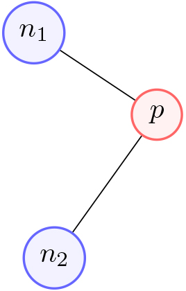

To find a winner using brute force, it requires $O(m)$ computations, where $m$ represents the number of neurons, for every data point. Assuming there are $n$ data points, if a learning epoch goes through the complete dataset and identifies a winner, then every epoch would need $O(mn)$ computations.

As we expand the map, additional neurons are incorporated into scale $m$ . To expedite this process, we employ a k-d tree to perform queries with an average time complexity of $O(\log{m})$ [16].

Hence, this approach typically requires $O(n\log{m})$ per epoch, which represents a significant advancement in terms of scalability for larger networks.

3.2.2 Adapt weights

Adapting weights is another essential characteristic of Self Organizing Maps. In this process, the weights are adjusted for all nodes within a certain distance from the winning node, which is determined using the weight adaptation rule outlined below. Figure 4 shows that neuron $n_{1}$ is the winning neuron. Additionally, we can see that since neuron $n_{2}$ is situated within a distance of $r$ from $n_{1}$ , its weight undergoes a change, whereas neuron $n_{3}$ remains unaffected.

Figure 4.

Neighborhood.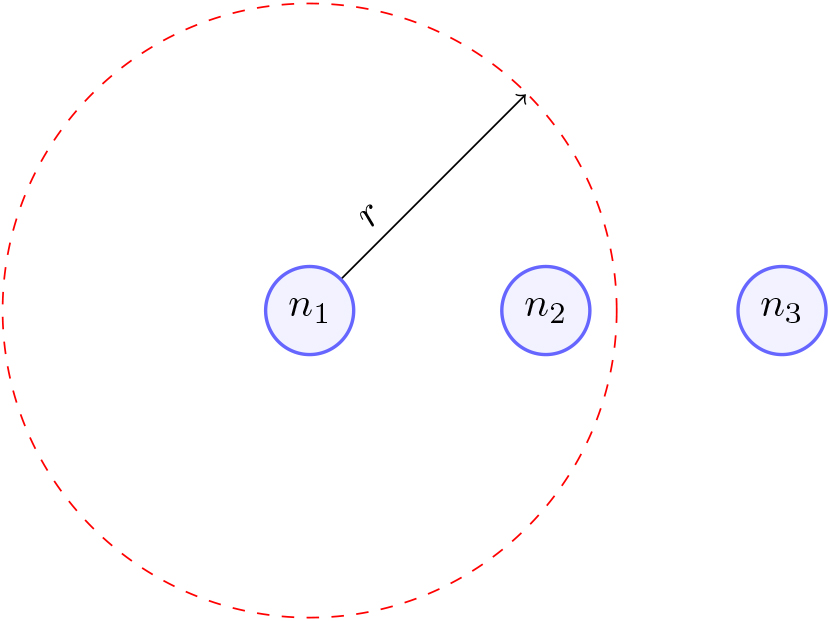

As can be seen in Algorithm 2, line 9, the iteration value $k$ is initialized to 0 and is incremented after processing each datapoint.

$\displaystyle n_{j}(k+1)=\left\{\begin{array}[]{ll}n_{j}(k)&n_{j}\notin M\\ n_{j}(k)+LR(k,N)\times d(n_{j},p)&n_{j}\in M\\ \end{array}\right.$ (3)

Where $n_{j}$ denotes the neuron’s weight, $M$ represents the set of neighboring neurons of the winning node. The learning rate is computed using the formula given below, as determined by $L R$ .

$\displaystyle LR(k,N)=0.02^{\lfloor\frac{1+k}{|N|}\rfloor}$ (4)

Here, $|N|$ signifies the total number of neurons in the network. It is obtained by raising this value to the floor of the ratio of the current iteration and $|N|$ .

3.2.3 Grow node

If the error exceeds the growth threshold, it indicates that the data point is not adequately covered within a specific radius of a neuron. Thus, we generate a new neuron and assign its weights to the corresponding data point.

$\displaystyle n_{\text{new}}=p_{i}$ (5)

At first, $n_{\text{new}}$ could be positioned inaccurately due to noise in a $p_{i}$ . However, with further learning iterations and smoothing, this point attains a more precise final weight. This is because the data cleaning stage has already revealed that more data points are situated within a specific range.

3.3 Connection rule

Once the node growth phase is completed and the terminal condition is reached, we apply the connection rule. We present each datapoint $p_{i}$ to trigger the connection rule. At each iteration, we identify the two neurons that are nearest to the input datapoint and connect them with an edge. This is based on the Hebbian learning principle, which suggests that “neurons that fire together wire together” [17].

As Fig. 5 shows, neurons $n_{1},n_{2}$ are nearer to datapoint $p$ than $n_{3}$ , which leads to linking $n_{1}$ and $n_{2}$ .

Figure 5.

Connection rule.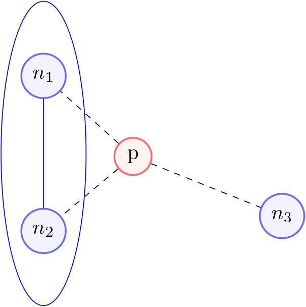

Figure 6.

Node collapse.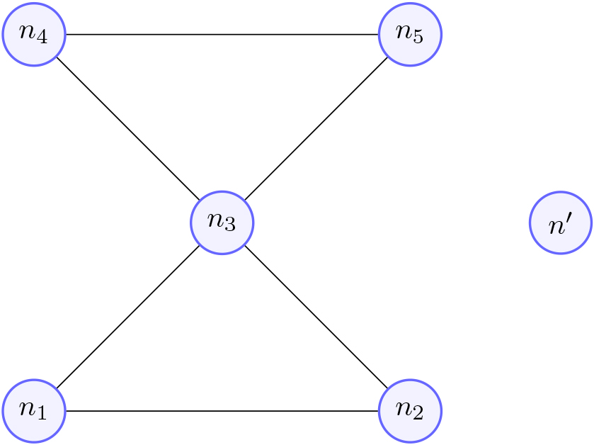

In order to determine the path connections between nodes, this rule utilizes the proximity of datapoints to nearby neurons. This guarantees a level of locality between two nodes with respect to other nodes. However, the rule does not take into account angle information, which could potentially enhance performance accuracy.

3.4 Collapsing

As this method tends to add an excess of edges, it can inadvertently lead to the creation of false triangular sub-graphs. To address this issue, the triangles are merged into a single point during this particular step.

To begin the process, we first list out all the nodes that form a triangle and then sort them based on their degree (i.e., number of edges). Then, the triangles that contain the node with the highest degree are collapsed iteratively. Assume there are neurons $n_{1},n_{2},n_{3},n_{4},n_{5}$ in the following formation. To simplify the graph, we collapse each edge into a single point. The weight of the new point is calculated by averaging the value of all the collapsed triangles’ nodes. In Fig. 6, we demonstrate the collapsing process with two interconnected triangles.

$\displaystyle n^{\prime}=\frac{\sum_{i\in T}n_{i}}{|T|}$ (6)

Here, $T$ denotes the set of nodes in the collapsed triangle.

3.5 Smoothing

Once the network has been contracted enough to eliminate triangular edges, it undergoes a weight adaptation phase. This phase is similar to the learning and growing step, but new growth is not permitted.

: Smoothing[1] SmoothingN, D, r $r_{\text{large}}\leftarrow r*2$ 50 Runs $p\in D$ winner, error $\leftarrow$ FindWinner (N, p) AdaptWeights (winner, $p$ , $r_{\text{large}}$ ) $r_{\text{small}}=r*0.5$ 50 Runs $p\in D$ winner, error $\leftarrow$ FindWinner (N, p) AdaptWeights (winner, $p$ , $r_{\text{small}}$ )

To accommodate newly contracted nodes in finding a general area they belong to, we increase the initial neighborhood size by two-fold. Following this, we apply the learning phase for a total of 50 iterations.

Subsequently, we reduce the neighborhood to half of the initial size to accurately position each node in its optimal location. This process is performed for each data point for a total of 20 iterations.

4. Results and comparison

When this method was created, it was meant for trail networks primarily. However, it is still important to compare its capabilities with existing approaches. Hence, we compared and evaluated our network with the Kernel Density Estimation (KDE) approach and the OSM datasets. These datasets are comprised of five different networks of GPS traces, as outlined in [2].

In order to evaluate different network construction techniques, benchmark metrics are designed by [2] including precision, completeness, and topological correctness. They have utilized Kernel Density Estimation from OSM traces for network construction and have reported the evaluation results. Our paper also includes a comparison of our method’s performance on these metrics using the same dataset.

To ensure the most accurate comparison of methods, we create and train a network for each GPS trace provided. Next, we calculate the precision, completeness (comp), and topological correctness (topo) metrics presented in Table 1, using the ground truth geometry as a reference.

4.1 Metrics

4.1.1 Segments

We utilize segments represented by $s$ for the metrics and their associated algorithms. We define a segment as a path between two nodes with a degree of one or greater than two in a graph.

Figure 7 presents us with a straightforward graph. The graph is divided into segments based on color, which is visible on the right. It is notable that when the orange nodes are connected to a segment, they are part of that segment. In total, this simple graph comprises six segments.

Moreover, it is essential to mention that every node in this graph is a shape point. The algorithms will denote it as $p\in s$ .

Figure 7.

Segments.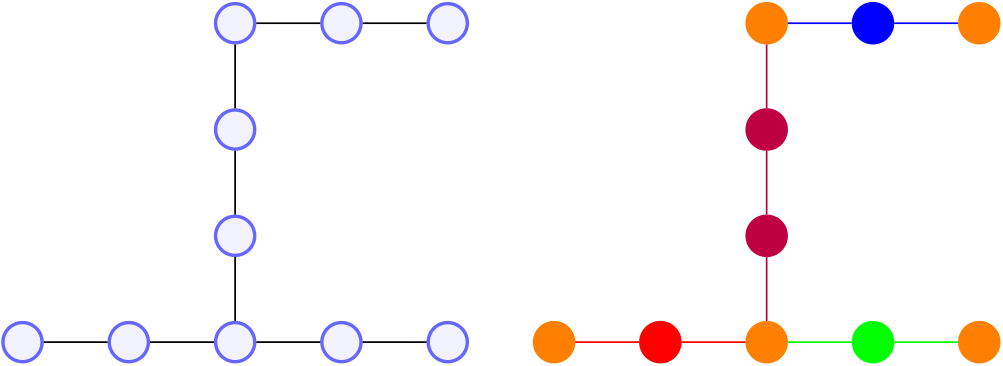

: Distance from point to line[1] LineDistance $p,n_{1},n_{2}$ $p$ datapoint, $n_{1},n_{2}$ forming a line $x_{0},y_{0}\leftarrow p[0],p[1]$ $x_{1},y_{1}\leftarrow n_{1}[0],n_{1}[1]$ $x_{2},y_{2}\leftarrow n_{2}[0],n_{2}[1]$ $\left|\frac{(x_{2}-x_{1})*(y_{1}-y_{0})-(x_{1}-x_{0})*(y_{2}-y_{1})}{(\sqrt{(x% _{2}-x_{1})^{2}+(y_{2}-y_{1})^{2}}}\right|$

4.1.2 Completeness

: Minimum distance from point to polyline[1] MinDistp, s $p\in s_{c},s\in T$

$\min\leftarrow$ inf $n_{1},n_{2}\in\text{zip}(s,s[1:])$ $d\leftarrow$ LineDistance $(p,n_{1},n_{2})$ See Alg. 7 $d<\min$ $\min\leftarrow d$ $\min$ zip returns a list of ordered pairs $\text{zip}(L,K)\rightarrow[(l_{1},k_{1}),(l_{2},k_{2}),\ldots,(l_{n},k_{n})]$ where $l_{i}\in L$ and $k_{i}\in K$

: Completeness[1] CompletenessT, C $s_{c}\in C$ $s_{t}\in T$ $n\leftarrow 0$ $\textit{SUM}\leftarrow 0$ $p_{c}\in s_{c}$ $\textit{SUM}+=\textit{dMin}(p_{c},s_{t})$ See Alg. 4.1.2 $n+=1$ $d_{ct}\leftarrow\textit{SUM}/n$ assign $s^{\prime}_{t}$ with smallest $d_{ct}$ $l=$ sum over all $s^{\prime}_{t}$ $L=$ sum over all $s_{t}$ $l/L$

When the completeness function calculates the percentage of the segments that match the ground truth network, without taking into account the accuracy of the matched segments.

We briefly describe the pseudo-code in Alg. 4.1.2.

We work with two main parameters: $T$ , which represents the ground truth network, and $C$ , which represents the constructed network. We iterate through each segment $s_{c}\in C$ and each segment $s_{t}\in T$ . Practically, for every segment, we search for the nearest segment in the ground truth network. We then evaluate the amount of total distance that is matched by the constructed network, which results in a score that always falls in the range of 0 to 1.

4.1.3 Precision

The precision function provides the mean distance of all matched segments, along with the standard deviation across all of the matched segments.

We describe a pseudo-code of this algorithm in Alg. 4.1.3. Similar to the completeness function, we iterate through each segment in the built network and search for the nearest segment in the ground truth network. At each shape point along the segments, we determine the distance and sum them up. This sum is then added to an overall precision array. Finally, we report the average distance across the entire array.

These scores give us an understanding of how erroneous the matched segments from the previous metric might be.

: Precision[1] PrecisionT, C $m=0$ $s_{c}\in C$ $s_{t}\in T$ $n\leftarrow 0$ $\textit{SUM}\leftarrow 0$ $p_{c}\in s_{c}$ $\textit{SUM}\leftarrow\textit{SUM}+\textit{dMin}(p_{c},s_{t})$ $n\leftarrow n+1$ $d_{ct}\leftarrow\textit{SUM}/n$ $m\leftarrow m+1$ assign $s^{\prime}_{t}$ to the $s_{t}$ with smallest $d_{ct}$ $m\leftarrow m+1$ precisionARRAY[m] $\leftarrow$ distance between $s_{c}$ and $s^{\prime}_{t}$ average and standard deviation of precisionARRAY

4.1.4 Topological correctness

To quantify the level of connection between the constructed and the ground truth networks, we use the topological correctness metric. We deploy the Floyd-Warshall algorithm to both the constructed network’s adjacency matrix $A_{c}$ and the ground truth adjacency matrix $A_{t}$ . This algorithm computes the shortest path between all pairs of vertices in a weighted graph [18]. Typically in impelentation, this results in a matrix where each element represents the total path cost between vertices. We then take an average of each returned matrix and produce the quotient as part of the topological correctness metric.

Figure 8.

Floyd-warshall.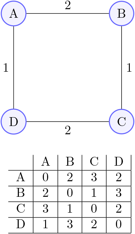

Figure 9.

Metrics across various spread factor values.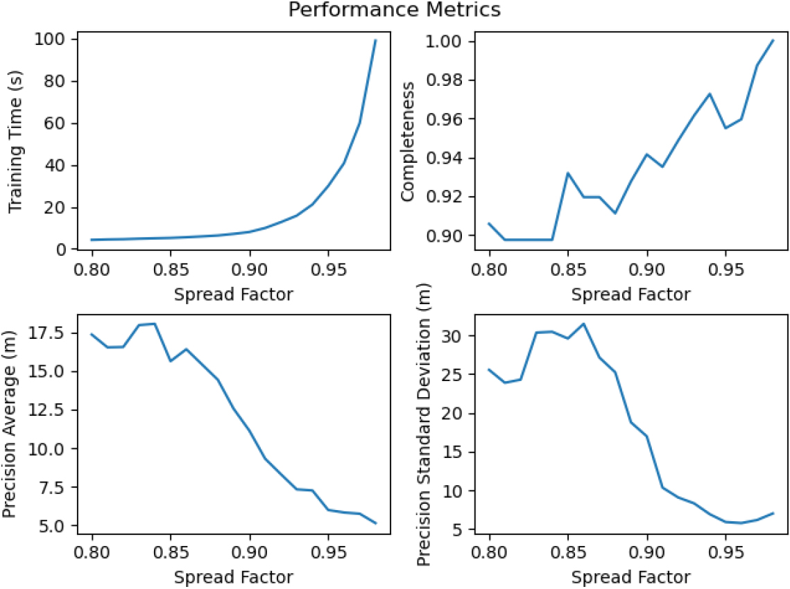

The Floyd-Warshall algorithm finds all pairs’ shortest path for a weighted graph [18]. In many implementations, this will be a matrix whose elements are the total path cost from one vertex to another. Then, we calculate the average of each returned matrix and generate the quotient. In Fig. 8, we demonstrate a simple example of the Floyd-Warshall algorithm on a graph with its result below.

Figure 10.

A portion of a constructed network from trace 1 at SF 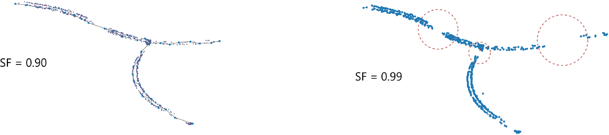$=$ 0.90 vs SF $=$ 0.99.

In $A_{t}$ and $A_{c}$ , $A$ is the adjacency matrix, $t$ denotes the ground truth network, and $c$ denotes the constructed network.

$\displaystyle F_{t}=\text{Floyd}(A_{t})$ $\displaystyle F_{c}=\text{Floyd}(A_{c})$ $\displaystyle a_{t}=\text{average value of non-diagonal elements in }F_{t}$ $\displaystyle a_{c}=\text{average value of non-diagonal elements in }F_{c}$ $\displaystyle topo=\frac{a_{t}}{a_{c}}$

An important consideration for the production of these networks is the choice of the SF. For a consistent way to choose a spread factor, we trained the network on each trace at spread factors from 0.80 to 0.99 at 0.01 intervals and analyzed the result graphs. Looking at Fig. 9, we see there is a time blow-up that occurs at SF $=$ 0.92. This choice seeks to be a middle ground between improved completeness and precision and degenerate graph construction. For sufficiently high values of SF, we see graphs with node clusters around points with large unconnected gaps between them. Whereas with a lower SF we get a more accurate representation of the graph. The SF value of 0.99, as we see in this figure, leads to a degenerate graph yet still has high completeness and precision. Comparison Fig. 10. In this graph, we have blue circles representing nodes and red circles representing the GPS data points used. In the first graph, with $SF=0.90$ , we see a well-constructed graph with meaningful topological connections. In the second graph, with $SF=0.99$ , we see many more neurons in our GSOM have been constructed because of the increased growth threshold value in Alg. 3.2. These many dense, unnecessary nodes lead to an inability to connect nodes together with our connection strategy, as seen by the gaps in connections.

4.2 Discussion

In Fig. 11, you can see the performance of our proposed approach based on the dataset from [2], comprising of different network traces. In Table 2, we see the individual metrics produced by our method and the difference to the reference data.

Considering the distinctive features of each network, we evaluate and compare the performance results across a network of traces. We can see some of the features in Table 1.

Table 1
GPS traces networks

Network	Total length (m)	# of nodes	# nodes per km²	Source	Traces
Net 1	32,245	42	2	OSM [19]	1, 2, 3, 4, 5, 6
Net 2	56,669	35	55	OSM [19]	7, 8, 9, 10, 11, 12
Net 3	34,595	65	9	GeoLife [20]	13, 14, 15, 16, 17, 18
Net 4	73,380	80	3	GeoLife [20]	19, 20, 21, 22, 23, 24
Net 5	11,695	151	508	Hashemi [2]	25, 26, 27, 28, 29, 30, 31, 32, 33

Figure 11.

Performance comparison with [2] with different network traces. The error results indicates the precision of the evaluated approach.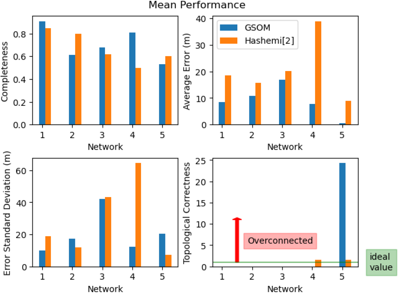

Table 2

GPS traces networks

NET	SF (%)	Completeness	Precision (m) average	Precision (m) standard deviation	Topological correctness	Time (s)
1	0.90	0.96 $+$ 0.09	9.35 $-$ 10.19	10.04 $-$ 9.27	0.00 0.00	9.44
1	0.92	0.98 $+$ 0.11	8.09 $-$ 11.45	10.37 $-$ 8.94	0.00 0.00	10.11
1	0.90	0.92 $+$ 0.09	11.20 $-$ 5.90	12.25 $-$ 5.10	0.00 0.00	2.34
1	0.93	0.88 $+$ 0.05	6.80 $-$ 11.21	8.48 $-$ 10.61	0.00 0.00	3.04
1	0.93	0.86 NA	8.39 NA	10.59 NA	0.00 NA	0.71
1	0.92	0.86 NA	6.72 NA	8.16 NA	0.00 NA	0.69
2	0.90	0.74 $-$ 0.09	11.83 $-$ 4.13	18.22 $+$ 5.19	0.00 0.00	25.82
2	0.93	0.79 $-$ 0.05	11.15 $-$ 4.07	21.68 $+$ 9.51	0.00 0.00	38.04
2	0.90	0.55 $-$ 0.21	13.84 $-$ 2.40	19.89 $+$ 8.22	0.00 0.00	4.65
2	0.92	0.61 $-$ 0.16	11.14 $-$ 4.37	15.02 $+$ 3.82	0.00 0.00	6.03
2	0.90	0.41 NA	13.20 NA	22.10 NA	0.00 NA	1.23
2	0.92	0.58 NA	4.34 NA	6.70 NA	0.00 NA	0.89
3	0.90	0.81 $+$ 0.14	14.07 $+$ 2.03	38.06 $+$ 20.77	0.00 0.00	10.16
3	0.90	0.80 $+$ 0.15	17.19 $-$ 2.26	84.68 $+$ 29.21	0.00 0.00	9.88
3	0.90	0.79 $+$ 0.22	7.28 $-$ 17.54	12.34 $-$ 37.72	0.00 0.00	0.29
3	0.91	0.70 $+$ 0.13	9.44 $-$ 15.38	20.15 $-$ 29.91	0.00 0.00	0.35
3	0.95	0.51 NA	20.08 NA	35.22 NA	0.00 NA	0.04
3	0.93	0.49 NA	32.90 NA	61.61 NA	0.00 NA	0.05
4	0.95	0.91 $+$ 0.26	4.25 $-$ 12.92	5.41 $-$ 29.74	0.00 1.11	1637.74
4	0.94	0.93 $+$ 0.26	4.05 $-$ 12.08	8.82 $-$ 24.65	0.00 1.05	682.89
4	0.88	0.85 $+$ 0.52	12.14 $-$ 49.17	26.11 $-$ 68.73	0.00 2.15	15.88
4	0.90	0.84 $+$ 0.51	8.07 $-$ 53.24	14.25 $-$ 80.59	0.00 2.15	27.40
4	0.87	0.69 NA	9.04 NA	9.24 NA	0.00 NA	1.40
4	0.88	0.64 NA	8.97 NA	10.91 NA	0.00 NA	1.71
5	0.95	0.46 $+$ 0.00	24.22 $+$ 12.93	20.64 $+$ 12.56	142.37 1.70	40.15
5	0.95	0.74 $-$ 0.10	14.64 $+$ 10.90	22.87 $+$ 19.04	58.22 1.11	30.04
5	0.94	0.70 $-$ 0.28	12.13 $+$ 11.03	16.98 $+$ 15.92	58.05 1.01	22.51
5	0.93	0.44 $+$ 0.01	18.82 $+$ 6.20	15.78 $+$ 6.02	112.32 1.83	8.01
5	0.92	0.50 $-$ 0.12	19.26 $+$ 12.94	17.03 $+$ 10.70	89.22 1.39	5.05
5	0.90	0.54 $-$ 0.24	21.61 $+$ 18.11	32.47 $+$ 27.17	93.74 0.00	4.42
5	0.90	0.48 $+$ 0.09	24.22 $+$ 8.78	34.31 $+$ 23.83	68.92 2.29	1.72
5	0.88	0.51 $+$ 0.12	26.90 $+$ 11.46	33.91 $+$ 23.43	90.57 2.29	1.09
5	0.87	0.44 $-$ 0.03	21.53 $+$ 10.60	24.89 $+$ 15.45	79.53 1.85	1.22

Figure 12.

Network traces.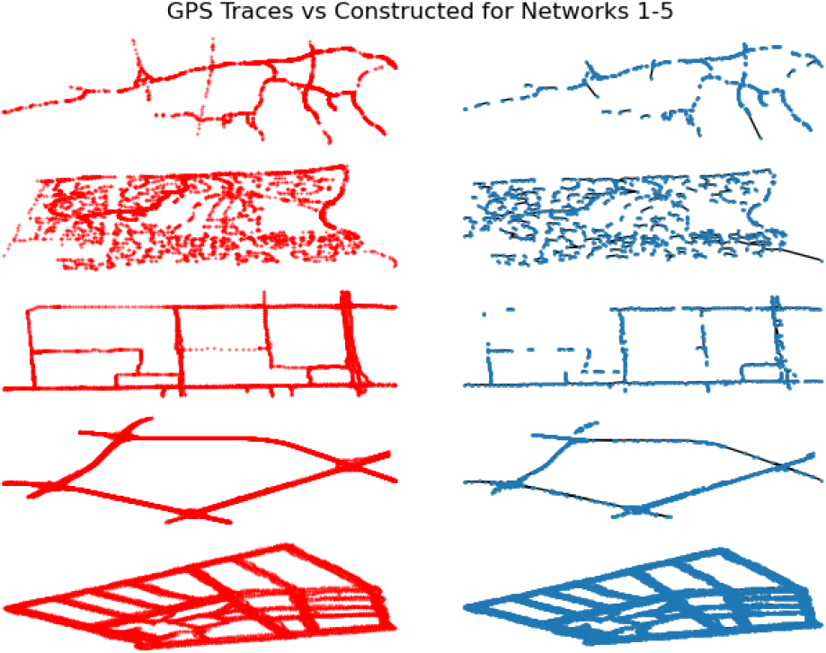

In comparison of our proposed GSOM approach to Hashemi’s KDE technique, we have observed superior overall performance for networks 1, 3, and 4. In addition, we have also improved some metrics of networks 2 and 5. In addition, Hashemi’s KDE approach could not for a network on multiple trajectories in the aforementioned networks, as indicated by NA (See Table 1). On the other hand, our approach constructs these networks, albeit with lower accuracy levels in many of the metrics, compared to the other traces from that network set. This contributes to a lower average performance for our approach.

In general, our approach demonstrate consistent superiority in terms of completeness, precision, and standard deviation precision. However, our GSOM method falls short in terms of topological correctness with 0 results for four of the networks, indicating at least one connection in the constructed network in missing.

Although the KDE technique shows three networks that have a topological correctness of zero, the other two have an acceptable score near one, which is the ideal value. On the other hand, our method has a non-zero score on one network, but the average score is 24.32, implying that it generates an excessive number of connections.

In network 1, we see an improvement in all metrics. Notably, this network features the lowest density at two nodes per km² with a total length of 32,245 meters. The average times to perform our algorithm ranged from 2.34 seconds to 10.11 seconds.

In network 2, there is a moderate decrease in completeness but an improvement in average precision. However, with a worse standard deviation, a few segments were much more erroneous than most. Interestingly, this network has the second highest density, with 55 nodes per km² and a total length of 56,669 meters.

Again, we see an improvement in every category for network 3, with slightly improved completeness and smaller errors in precision. With a density of 9 nodes per km² this network is among the most sparse in these datasets. The total length is also similar to network 1 at 34,595 meters.

With network 4, there is an improvement in completeness and precision. However, our method fails to produce a non-zero value for topological correctness, while the KDE method does. Among the lowest densities at 3 nodes per km², this network is the longest at a total length of 73,380 meters.

Lastly, for network 5, our method does produce slightly worse completeness values. Our average precision is much lower; however, the standard deviation is much higher, which indicates that a small percentage of our constructed segments were highly inaccurate, but most were more precise. This network has the most unique characteristic, with the highest density of 508 nodes per km² and a total length of 11,695 meters. So this is a much smaller network in scale but with the highest total number of nodes at 151.

In sum, compared to the existing technique [2], our proposed method provides better average error and topological correction across all networks and better completeness and error standard deviation in most cases. However, the evaluation results indicate that our proposed approach works best in low-density networks and provides comparable and, in some cases, worse results in high-density networks.

5. Conclusion

Our paper introduced a new approach for building trail maps that performs similarly to the state-of-the-art methods. We evaluated the performance using various metrics that are now widely used as a standard in this field. It is worth noting that these standardized metrics are fairly new and in the past, many techniques were published using different testing methods, making it challenging to compare the results.

Based on the results, it is evident that this method has yielded encouraging outcomes. In comparison to previous techniques like KDE, we have observed improvements in trace analysis of several networks. Moreover, this method surpasses the current methodology in constructing trail maps, which was our original objective.

The main advantage of this work is the utilization of anonymized traces, allowing application to datasets that have been privatized. Reducing each iteration to scale linearly with input size is a major speed-up that allows the method to be used on even larger datasets. However, it faces challenges with edge prediction in densely geographic networks.

Future research may aim at enhancing edge prediction through more robust similarity metrics. $\beta$ skeletons might be a fitting approach for edge prediction. To make the model more robust against noise, advanced denoising techniques could be applied to boost performance.

References

Karimi

Kasemsuppakorn

. Pedestrian Network Map Generation Approaches and recommendation. International Journal of Geographical Information Science. 2013; 27(5): 947–962.

Hashemi

. A testbed for evaluating network construction algorithms from GPS traces. Computers, Environment and Urban Systems. 2017; 66: 96–109.

Kumar

Kalra

Dhande

. Curve and surface reconstruction from points: An approach based on self-organizing maps. Applied Soft Computing. 2004; 5(1): 55–66.

Yun

Uchimura

. Using self-organizing map for road network extraction from ikonos imagery. International Journal of Innovative Computing, Information and Control. 2006; 641–656.

Schwartz

Montero Jimenez

Salaün

Vingerhoeds

. A fault mode identification methodology based on self-organizing map. Neural Computing and Applications. 2020; 32(17): 13405–13423.

Forest

Lebbah

Azzag

Lacaille

. Deep embedded self-organizing maps for joint representation learning and topology-preserving clustering. Neural Computing and Applications. 2021; 33(24): 17439–17469.

Chao

Hua

Mao

Zhou

. A survey and quantitative study on map inference algorithms from GPS trajectories. IEEE Transactions on Knowledge and Data Engineering. 2020; 1–1.

Karagiorgou

Pfoser

. On vehicle tracking data-based road network generation. Proceedings of the 20th International Conference on Advances in Geographic Information Systems. 2012.

Liu

Biagioni

Eriksson

Wang

Forman

Zhu

. Mining large-scale, sparse GPS traces for map inference. Proceedings of the 18th ACM SIGKDD International Conference on Knowledge Discovery and Data Mining. 2012.

10.

Singh

Garg

. Automatic road extraction from high resolution satellite image using adaptive global thresholding and morphological operations. Journal of the Indian Society of Remote Sensing. 2012; 41(3): 631–640.

11.

Tao

Wang

. Spatial information inference net: Road extraction using road-specific contextual information. ISPRS Journal of Photogrammetry and Remote Sensing. 2019; 158: 155–166.

12.

Corbane

Syrris

Sabo

Politis

Melchiorri

Pesaresi

, et al. Convolutional Neural Networks for global human settlements mapping from sentinel-2 satellite imagery. Neural Computing and Applications. 2020; 33(12): 6697–6720.

13.

Stanojevic

Thirumuruganathan

Chawla

Filali

Aleimat

. Kharita: Robust Map Inference using Graph Spanners. arXiv. 2017 Feb.

14.

Yang

Tang

Ren

Chen

Xie

. Pedestrian network generation based on crowdsourced tracking data. International Journal of Geographical Information Science. 2019; 34(5): 1051–1074.

15.

Buchin

Gudmundsson

Hendriks

Sereshgi

Sacristán

, et al. Improved map construction using Subtrajectory clustering. Proceedings of the 4th ACM SIGSPATIAL Workshop on Location-Based Recommendations, Geosocial Networks, and Geoadvertising. 2020.

16.

Bentley

. Multidimensional binary search trees used for associative searching. Communications of the ACM. 1975; 18(9): 509–517.

17.

Marsland

. Machine learning: An algorithmic perspective. CRC Press; 2011.

18.

Floyd

. Algorithm 97: Shortest path. Communications of the ACM. 1962; 5(6): 345.

19.

Available from: https://www.openstreetmap.org/.

20.

Available from: https://www.microsoft.com/en-us/research/project/geolife-building-social-networks-using-human-location-history/.