Novel deep learning architectures for haemodialysis time series classification

Abstract

Classifying haemodialysis sessions, on the basis of the evolution of specific clinical variables over time, allows the physician to identify patients that are being treated inefficiently, and that may need additional monitoring or corrective interventions. In this paper, we propose a deep learning approach to clinical time series classification, in the haemodialysis domain. In particular, we have defined two novel architectures, able to take advantage of the strengths of Convolutional Neural Networks and of Recurrent Networks. The novel architectures we introduced and tested outperformed classical mathematical classification techniques, as well as simpler deep learning approaches. In particular, combining Recurrent Networks with convolutional structures in different ways, allowed us to obtain accuracies above 81%, coupled with high values of the Matthews Correlation Coefficient (MCC), a parameter particularly suitable to assess the quality of classification when dealing with unbalanced classes-as it was our case. In the future we will test an extension of the approach to additional monitoring time series, aiming at an overall optimization of patient care.

Keywords

Time series classification deep learning convolutional Networks recurrent networks haemodialysis

1. Introduction

End stage renal disease patients are affected by a severe condition, which necessarily requires haemodialysis treatment.

Haemodialysis, to be repeated 3/4 times a week, removes water in excess and clears the patient’s blood from metabolites. During the tratment, the patient is continuosly monitored, by sampling different physiological variables, which are therefore acquired and logged in the form of time series. Among them, the Haematic Volume (HV), strictly correlated with water extraction, is particularly important. Specifically, the HV time series should start with an exponential decreasing trend, and then it should register a milder, linear decreasing trend. A different behaviour, such as a linear decreasing trend since the beginning, or sudden slope changes, indicates an insufficient water extraction [1], that may suggest the presence/insurgence of haemodynamic instability, or of cardiovascular problems [2, 3].

The capability to classify HV time series as problematic versus normal is therefore extremely relevant to quickly identify issues, and to optimize patient’s therapy.

Classical approaches to time series classification require a dimensionality reduction step (often obtained by means of mathematical transforms, such as the Discrete Fourier Transform [4], or the Discrete Cosine Transform [5]), followed by the use of a classifier (such as, e.g., a Support Vector Machine [6]) in the reduced feature space.

In this paper, on the other hand, we suggest the adoption of a different strategy, that exploits deep learning [7].

In particular, we have defined two novel, complex deep learning architectures, which differently combine elementary modules whose strength has already been shown in the literature. Specifically, our novel architectures exploit the sinergy of Convolutional Neural Network modules and of Recurrent Neural Network ones.

In the following, we will illustrate the networks details and present our experiments, that have demonstrated the feasibility of the approach, able to overcome simpler techniques.

The paper is organized as follows: In Section 2 we present background and related work; Section 3 illustrates the proposed deep learning architectures; Section 4 provides experimental results. Section 5 is devoted to discussion, conclusions and future work.

2. Background and related work

Deep learning techniques [7], after proving particularly successfull in computer vision (see, e.g., [8]), have started to be applied to time series classification (see, e.g., [9, 10, 11, 12, 13, 14].

In this section, we will present some basic deep learning architectures that will be used as elementary modules in our approach.

2.1 Convolutional Neural Networks

Convolutional Neural Networks (CNNs) take inspiration from the animal visual cortex organization [15], where individual neurons respond to stimuli only in a restricted region of the visual field, and the regions related to different neurons partially overlap, such that, globally, the entire visual field is covered. In CNNs, hidden layers perform convolutions: After passing through a convolutional layer, the input is abstracted to a feature map; the feature map is typically passed to a pooling layer, able to further reduce dimensionality.

Convolution and pooling layers can be stacked; fully connected layers typically complete the architecture and output the class.

Composed of sparse connections with tied weights, CNNs have significantly fewer parameters than a fully connected network of similar size [16].

One-dimensional CNNs are particularly suitable for time series data. As a matter of fact, they can model local dependencies that may exist between adjacent data points [17], and can capture how the input evolves over time [18].

CNNs for time series classification have been proposed, e.g., in [19, 20, 13], and are the most popular deep learning approach in physiological signals classification, as reported in a recent survey [12].

We also obtained encouraging results in medical time series classification resorting to CNN in our previous work [14].

2.2 Recurrent Networks

Recurrent Neural Networks (RNNs) [21] are Neural Networks specialised for processing sequential data. The idea in RNNs is to preserve the results of previous calculations with memories, i.e., with feedback connections that provide a parameter sharing across different parts of the model. Specifically, the hidden layer in the RNNs considers both the current input and the results of the last hidden layer, unlike traditional Neural Networks where there is no dependency between the calculation results.

In order to achieve long-term memory, the RNN model requires a significant amount of model training time. Normalization (a process by which the inputs are linearly transformed to have zero mean and unit variance) can be applied to accelerate training. However, in the case of RNNs some of the inputs of the $n$ th layer are from the $(n-1)$ th layer, and are not raw inputs: as the training progresses, the effect of normalization thus reduces, causing the vanishing gradient problem [22], which can slow down the entire training process and cause saturation. The Long Short Term Memory Network (LSTM, [22]) architecture has been proposed in order to shorten the training time, and to deal with the vanishing gradient problem. The core idea in LSTMs is to introduce a cell state, more complex than the memory cell in basic RNNs, where information can be added or removed by gated structures, composed of a sigmoid layer and a multiplication operation [22].

LSTMs can process time series data, since they can potentially learn the complex dynamics within the temporal ordering of input sequences as well as use the internal memory to remember information across input sequences. However, the performance of LSTMs can be reduced due to rapid overfitting in small short-sequence datasets, and LSTMs can fail to learn long-term dependencies in larger long-sequence datasets. In order to deal with these difficulties, a dimension shuffle layer can be introduced [23]. This layer transposes the temporal dimension of the time series: a univariate time series of length $n$ will be viewed as a multivariate time series (having $n$ variables) with a single time step. Training time will be reduced as well [23].

Gated Recurrent Units (GRUs) [24] are lighter versions of RNNs with respect to standard LSTMs in term of topology, computation cost and complexity. The GRU requires fewer network parameters, which makes the model faster. On the other hand, LSTM can provide better performance, when enough computational power is available [24].

2.3 Combined architectures

The combined use of CNNs with RNNs is also being investigated.

An interesting example is represented by the Chrono-Net architecture [25], able to support electroencephalography time series classification.

ChronoNet is formed by stacking multiple one-dimensional convolution layers followed by GRU layers, where each convolution layer uses multiple kernels of exponentially varying lengths and the stacked GRU layers are densely connected, i.e., each GRU layer is connected to every other GRU layer in a feed-forward manner. This choice mitigates the problem of the vanishing gradient. ChronoNet has outperformed the best previously reported accuracy on an experimental dataset.

Other examples of composite architectures can be found in image interpretation. The paper in [26], for instance, presentes a two-parallel-branch deep Neural Network able to predict pixel-wise gland segmentation and contour jointly. The architecture constitues a co-learning framework for the two learning tasks. However, since such works are not focused on time series, they are only loosely related to our contribution.

3. Material and methods

In this section, we technically describe the deep learning architectures we have proposed and tested. While Section 3.1 presents our implementation of a “classical” LSTM network, in Section 3.2 we describe two novel architectures, able to combine LSTMs and convolutional modules. Specifically, the architecture in Section 3.1 is used as a building block of the architectures in Section 3.2. Details are provided in the following.

3.1 LSTM-based classification

Our basic LSTM architecture, depicted in Fig. 1, exploits a dimension shuffle block, as described and motivated in Section 2. Then, the actual LSTM block is composed of 256 units with $t a n h$ activation function and is followed by a dropout layer, which randomly forces a fraction of the input units to be ignored at each update during training time, to help prevent overfitting [27]. The final layer is a sigmoid layer. Hyperparameters were set experimentally, as explained in Section 4.

Figure 1.

LSTM-based classification architecture.

Figure 2.

Composing CNN and LSTM: Architecture 1.

Figure 3.

Composing CNN and LSTM: Architecture 2.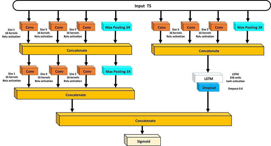

3.2 Composing LSTM and CNN: Novel deep learning architectures

Besides the classical architecture described in the previous subsection, we also propose two novel ones, able to combine convolutional modules with LSTMs, with the aim of taking advantage of the strengths of both.

Specifically, in Architecture 1 (see Fig. 2) we have put a convolutional branch in parallel with an LSTM branch. The convolutional branch, in turn, is made by three convolutional modules, each one using three convolutions with kernels of sizes 1, 3, and 5, and a parallel path which implements a 3 max-pooling operation (see also [28]). The three modules are articulated in two layers: one module on the first layer, and the other two on the second layer, as illustrated in the figure. The LSTM branch, on the other hand, is built as the one described in Subection 3.1.

In this architecture, the two branches perceive the input in two different views. The convolutional branch views the input time series as a univariate time series with multiple time steps, and tests different kernels; a second layer further exploits the power of convolution. The LSTM branch views the input time series as a multivariate time series with a single time step, thanks to the dimension shuffle mechanism.

The two branches are then concatenated. The final layer is a sigmoid layer.

In Architecture 2, on the other hand, we have placed two convolutional modules as the one described above on the first layer. Then, two parallel branches develop on the second layer: the first branch contains another analogous convolutional module, while the second one exploits LSTM. In this way, an already compressed input is provided to the LSTM branch, in order to reduce computation time. In this case dimension shuffle is not applied. The two branches are then concatenated, and a sigmoid layer completes the architecture. The rationale for proposing to place the convolutional module before the two parallel branches is two-fold. First, it reduces the input vector’s length. This becomes relevant when reaching the LSTM layer, which during training constitutes the most computationally expensive part of the network. Second, convolution extracts local information from neighboring time points, a first step towards learning temporal dependencies. Then, the LSTM layer is responsible for capturing both short and long-term dependencies. This architecture is shown in Fig. 3.

Hyperparameters were set experimentally, as explained in Section 4.

4. Results

Our input HV time series were recordings of 240 samples on average, with a sampling time of 1 minute. We truncated longer series, and added zeros to extend shorter series. We worked with a dataset of 5376 time series, belonging to 74 different patients (72 series per patient on average, varying from 1 to 280).

Our classification was a binary one: Class 1 refers to negative cases, i.e., non-problematic situations, where an exponential HV decrease is followed by a linear decrease; class 0, on the other hand, refers to positive cases, i.e., problematic situations where this ideal behaviour is not met, due to a slower decrease, or to sudden slope changes.

We performed the labeling process in two steps: First, each time series was de-noised through wavelet transform and its gradient was calculated over time to apply a first temporary label; then, the labeled time series were validated by medical experts to confirm or to correct the automatically assigned labels on the basis of domain knowledge. At the end of the process, 3680 negative cases and 1696 positive cases were made available.

For our experiments, we divided our datasets in two parts: 70% of the data where used for training, and 30% for test. On training data, we performed a 10 fold cross validation, in order to choose the hyperparameter values that give the lowest cross validation average error. In the end, the following hyperparameter values were set: Batch size $=$ 32; learning rate $=$ 0.01; model optimizer $=$ Adam; losses $=$ binary cross entropy.

Experiments were conducted by resorting to the TensorFlow tool1. We exploited a machine with the following characteristics: Operating System: Windows Server 2012 R2; Processor: Intel Xeon E3-12xx v2 (Ivy Bridge, IBRS) 2.70 GHz (2 processors); Installed memory (RAM): 8.00 GB; System Type: 64-bit Operating System, 64-based processor; Hard disk memory: 40 GB.

The number of parameters of the three different architectures is summarized in Table 1. As it can be observed, the LSTM-based architecture has less parameters than the composite ones (i.e., Architecture 1 and Architecture 2). We also tested a more complex LSTM network, with 128 additional units (on a second LSTM layer), which had a similar number of parameters with respect to Architecture 2 (see Table 1). With this choice, however, computational efficiency dropped drastically, making the solution unfeasible.

Table 1
Number of parameters of the tested architectures

LSTM	LSTM 256 $+$ 128 units	Architecture 1	Architecture 2
264449	461441	386593	405553

In the tables below, we report results on test set, at different epochs (up to 200). The results are reported by class, and the average values, weighted by the number of instances in the classes, are calculated as well. MCC, K-statistics and accuracy are not related to a single class, therefore we provide them only as overall results.

The LSTM-based architecture (Fig. 1) reached an accuracy of 74%, coupled with a Matthews Correlation Coefficient (MCC, a parameter particularly suitable to assess the quality of classification when dealing with unbalanced classes, which should be ideally close to 1) of 0.35. The complete results are shown in Table 2.

Table 2

Experimental results obtained by the LSTM-based architecture (Fig. 1)

Epochs	Class	Precision	Recall	F1-score	MCC	K-stat	Accuracy
50	0 (pos)	0.610	0.360	0.450
50	1 (neg)	0.750	0.890	0.820
50	w. ave	0.710	0.720	0.700	0.299	0.281	0.724
100	0 (pos)	0.630	0.320	0.420
100	1 (neg)	0.740	0.910	0.820
100	w. ave	0.710	0.730	0.700	0.295	0.269	0.726
150	0 (pos)	0.640	0.300	0.410
150	1 (neg)	0.740	0.920	0.820
150	w. ave	0.710	0.730	0.690	0.293	0.563	0.727
200	0 (pos)	0.770	0.280	0.410
200	1 (neg)	0.740	0.960	0.840
200	w. ave	0.750	0.750	0.700	0.354	0.293	0.747

Table 3

Experimental results obtained by Architecture 1 (Fig. 2)

Epochs	Class	Precision	Recall	F1-score	MCC	K-stat	Accuracy
50	0 (pos)	0.660	0.470	0.550
50	1 (neg)	0.780	0.890	0.830
50	w. ave	0.740	0.760	0.740	0.398	0.388	0.756
100	0 (pos)	0.610	0.690	0.650
100	1 (neg)	0.850	0.800	0.820
100	w. ave	0.770	0.760	0.770	0.469	0.467	0.762
150	0 (pos)	0.720	0.700	0.710
150	1 (neg)	0.860	0.870	0.870
150	w. ave	0.820	0.820	0.820	0.577	0.577	0.816
200	0 (pos)	0.740	0.640	0.690
200	1 (neg)	0.850	0.900	0.870
200	w. ave	0.810	0.820	0.810	0.563	0.560	0.818

Table 4

Experimental results obtained by Architecture 2 (Fig. 3)

Epochs	Class	Precision	Recall	F1-score	MCC	K-stat	Accuracy
50	0 (pos)	0.610	0.470	0.530
50	1 (neg)	0.780	0.860	0.820
50	w. ave	0.720	0.740	0.730	0.357	0.351	0.737
100	0 (pos)	0.700	0.310	0.430
100	1 (neg)	0.750	0.940	0.830
100	w. ave	0.730	0.740	0.710	0.339	0.298	0.742
150	0 (pos)	0.620	0.470	0.540
150	1 (neg)	0.780	0.870	0.820
150	w. ave	0.730	0.740	0.300	0.368	0.362	0.742
200	0 (pos)	0.660	0.710	0.690
200	1 (neg)	0.860	0.830	0.850
200	w. ave	0.800	0.800	0.800	0.538	0.537	0.796

Architecture 1(Fig. 2) and Architecture 2 (Fig. 3) worked better then the previously commented one. In particular, Architecture 1 (see Table 3) reached an accuracy of more than 81%, and an MCC of 0.56. Architecture 2 (see Table 4 had a comparable (actually, slightly poorer) performance (accuracy $=$ 79.6%, MCC $=$ 0.53). Generally speaking, both solutions performed well on our data set, already reaching promising results at 200 epoches.

For the sake of completeness, we also tested a pure CNN-based architecture, which, however, did not outperform the LSTM-based one (namely, at 200 epochs, the CNN-based architecture obtained an accuracy of 69%, coupled with a very low MCC value, specifically 0.18).

Moreover, we tested a composite (but simpler) architecture, composed just by the right-hand parallel branch of Architecture 2 (i.e., a CNN module followed by LSTM, see Fig. 3). This architecture’s performance, however, was not as satisfactory as the one of Architecture 2: At 200 epochs it provided an accuracy of 77%, and an MCC of 0.45.

We also compared the results presented above with the ones of a more classical approach, where we resorted to a mathematical transform for feature extraction, and to a Support Vector Machine (SVM) [6] for classification (Pearson VII function-based universal kernel and automatic search for the best complexity parameter). Namely, we adopted the Discrete Fourier Transform (DFT) [4] for feature extraction. DFT operates by decomposing the input into its constituent sine and cosine waves, and returns an ordered sequence of coefficients, where the most important information is concentrated at the lower indices of the sequence itself. In particular, we extracted the first 5 DFT coefficient for each time series (notably, the following coefficients were close to 0). We provided the coefficients to the SVM. The tests were performed using the open source tool Weka [29].

As reported in Table 5, the SVM using the 5 DFT coefficients obtained poor results. In particular, this model failed in identifying the positive cases, making it almost useless in a real environment. Furthermore, the very low value of the MCC suggests that this model is not far from a random predictor.

Table 5

Results obtained by the SVM classifier using 5 DFT coefficients

Class	Precision	Recall	F1-score
0 (positive)	0.75	0.19	0.31
1 (negative)	0.72	0.97	0.83
Weighted average	0.73	0.61	0.60
MCC	0.28
K-stat	0.20
Accuracy	0.73

In conclusion, Architecture 1 and Architecture 2, which are able to exploit the advantages of CNN and LSTM networks specificities in a synergistic way, proved to outperform a classical DFT-SVM approach, as well as several simpler deep learning architectures, that we considered in our experiments. In particular, the right-hand branch of Architecture 2, when implemented as a stand alone network, did not provide particularly satisfactory results: this finding could in part justify the slightly lower performance of Architecture 2 with respect to Architecture 1; on the other hand, the choice of defining two branches that perceive the input in two different views (a univariate time series with multiple time steps for the CNN-based branch, and a multivariate time series with a single time step for the LSTM branch), and operate in parallel as in Architecture 1, seems to be the optimal one.

5. Discussion and conclusions

HV time series classification can help physicians in identifying haemodialysis treatment inefficiency, allowing for early interventions that can lead to an overall optimization of patient care. Even if the final decision is always up to the medical expert, an automated tool can in fact help her to focus on critical situations, and speed up the decision process itself.

In this paper, we have proposed two novel deep learning architectures for HV classification.

Our experiments have proved the feasibility of the approach, which has outperfomed a more classical technique, based on DFT for feature extraction, followed by SVM for classification, as well as simpler deep learning networks.

The novel architectures, featuring a set of convolutional modules, differently combined with and LSTM-based branch, provided very good results, reaching an accuracy of about 80%. Moreover, both precision and recall results were high, with a very few unrecognized critical cases, thus guaranteeing a safe application in a medical domain.

The good classification performance is probably due to the fact that the developed deep learning models are able to capture the distinctive features from the HV time series, paying attention both to local and global temporal dependencies. In this case, the networks can be trained from these learned features even without big data [12], as in our experiments.

Moreover, the choice of defining two parallel branches that perceive the input in two different views (a univariate time series with multiple time steps versus a multivariate time series with a single time step), as in Architecture 1, seems to be the optimal one, at least in the case of HV classification.

In the future, we plan to conduct additional experiments, by extending the approach to other haemodialysis time series variables as well, in order to further evaluate and compare our novel deep learning architectures. We will also verify whether a stratification of time series on the basis of patient gender or age can provide an improvement in classification performance. Complete classification results, in turn, will lead to a personalization and an optimization of the haemodialysis patient management process.

Finally, from a methodological viewpoint, we will also consider transformer networks, which are being proposed in time series forecasting (see, e.g., [30]). Transformer networks exploit an encoder network, which encodes the input data based on a particular pattern, and a decoder network, that decodes the encoded input to produce the desired output. Such models use the mechanism of self-attention to boost training, and are particularly suited to manage long-term temporal dependencies. We will investigate whether such an approach can be useful also for time series classification, in our medical domain.

Author contribution

Conceptualization: G. Leonardi and S. Montani.

Methodology: S. Montani.

Software: M. Striani.

Validation: G. Leonardi and M. Striani.

Data curation: G. Leonardi and M. Striani.

Writing, original draft preparation: S. Montani.

Writing, review and editing: G. Leonardi, S. Montani and M. Striani.

Supervision: S. Montani.

Funding

This research has a financial support of the University of Piemonte Orientale.

Footnotes

https://www.tensorflow.org/.

Acknowledgments

The authors are grateful to Dr. Roberto Bellazzi for having provided medical knowledge.

Conflict of interest

The author declares no conflict of interest.

References

Santoro

Mancini

Zucchelli

. Ultrafiltration behaviour with different dialysis schedules. Nephrology, Dialysis, Transplantation: official Publication of the European Dialysis and Transplant Association – European Renal Association. 1998; 2(13 Suppl 6): 55-61.

Krepel

Nette

Akcahuseyin

Weimar

Zietse

. Variability of relative blood volume during hemodialysis. Nephrology, Dialysis, Transplantation: Official publication of the European Dialysis and Transplant Association – European Renal Association. 2000; 5(15): 673-9.

Titapiccolo

Ferrario

Garzotto

Cruz

Moissl

Tetta

, et al. Relative Blood Volume Monitoring during Hemodialysis in End Stage Renal Disease Patients. Conference proceedings: Annual International Conference of the IEEE Engineering in Medicine and Biology Society IEEE Engineering in Medicine and Biology Society Conference. 2010; (8): 2010: 5282-5.

Agrawal

Faloutsos

Swami

. Efficient similarity search in sequence databases. In: Lomet

, Editor, Proc 4th Int Conf of Foundations of Data Organization and Algorithms, Springer-Verlag, Berlin. 1993; pp. 69-84.

Strang

. The Discrete Cosine Transform. SIAM Rev. 1999; 41(1): 135-147.

Steinwart

Christmann

. Support Vector Machines. Springer Publishing Company, Incorporated. 2008.

LeCun

Bengio

Hinton

. Deep learning. Nature. 2015; 521(7553): 436-444.

Zhao

Wan

Sekuboyina

Tetteh

, et al. Knowledge-Aided Convolutional Neural Network for Small Organ Segmentation. IEEE Journal of Biomedical and Health Informatics. 2019; 23(4): 1363-1373.

Längkvist

Karlsson

Loutfi

. A review of unsupervised feature learning and deep learning for time-series modeling. Pattern Recognition Letters. 2014; 42: 11-24.

10.

Wang

Sun

Liu

. Adaptive Intelligent Control of Nonaffine Nonlinear Time-Delay Systems With Dynamic Uncertainties. IEEE Trans Systems, Man, and Cybernetics: Systems. 2017; 47(7): 1474-1485.

11.

Zhao

Shi

Zheng

Zhang

. Intelligent Tracking Control for a Class of Uncertain High-Order Nonlinear Systems. IEEE Trans Neural Netw Learning Syst. 2016; 27(9): 1976-1982.

12.

Faust

Hagiwara

Hong

Lih

Acharya

. Deep learning for healthcare applications based on physiological signals: A review. Computer Methods and Programs in Biomedicine. 2018; 161: 1-13.

13.

Sani

Wiratunga

Massie

Cooper

. KNN Sampling for Personalised Human Activity Recognition. In: Aha

Lieber

, Editors, Case-Based Reasoning Research and Development – 25th International Conference, ICCBR 2017, Trondheim, Norway, June 26-28, 2017, Proceedings. vol. 10339 of Lecture Notes in Computer Science. Springer. 2017; pp. 330-344.

14.

Leonardi

MSG

Montani

. Deep learning for haemodialysis time series classification. In: Proc R4HC/ProHealth and TEAAM Workshops, LNCS (to Appear), Springer, 2019.

15.

Matsugu

Mori

Mitari

Kaneda

. Subject independent facial expression recognition with robust face detection using a convolutional neural network. Neural Networks. 2003; 16(5-6): 555-9.

16.

Alom

Taha

Yakopcic

Westberg

Sidike

Nasrin

, et al. A State-of-the-Art Survey on Deep Learning Theory and Architectures. Electronics. 2019; 8(3).

17.

Wang

Yan

Oates

. Time series classification from scratch with deep neural networks: A strong baseline. In: 2017 International Joint Conference on Neural Networks, IJCNN 2017, Anchorage, AK, USA, May 14-19, 2017. IEEE. 2017; pp. 1578-1585.

18.

Lea

Vidal

Reiter

Hager

. Temporal Convolutional Networks: A Unified Approach to Action Segmentation. In: Hua

Jégou

, Editors, Computer Vision – ECCV 2016 Workshops – Amsterdam, The Netherlands, October 8-10 and 15-16, 2016, Proceedings, Part III. vol 9915 of Lecture Notes in Computer Science. 2016; pp. 47-54.

19.

Cui

Chen

. Multi-Scale Convolutional Neural Networks for Time Series Classification. CoRR. 2016; abs/1603.06995.

20.

Fan

Yao

Cai

Miao

Sun

. Multiscaled Fusion of Deep Convolutional Neural Networks for Screening Atrial Fibrillation From Single Lead Short ECG Recordings. IEEE J Biomedical and Health Informatics. 2018; 22(6): 1744-1753.

21.

Pascanu

, Cho

Bengio

. How to Construct Deep Recurrent Neural Networks. In: Bengio

LeCun

, editors, 2nd International Conference on Learning Representations, ICLR 2014, Banff, AB, Canada, April 14-16, 2014, Conference Track Proceedings. 2014.

22.

Hochreiter

Schmidhuber

. Long Short-Term Memory. Neural Computation. 1997; 9(8): 1735-1780.

23.

Karim

Majumdar

Darabi

Chen

. LSTM Fully Convolutional Networks for Time Series Classification. IEEE Access. 2018; 6: 1662-9.

24.

Józefowicz

Zaremba

Sutskever

. An Empirical Exploration of Recurrent Network Architectures. In: Bach

Blei

, Editors, Proceedings of the 32nd International Conference on Machine Learning, ICML 2015, Lille, France, 6-11 July 2015. 2015; pp. 2342-2350.

25.

Roy

Kiral-Kornek

Harrer

. ChronoNet: A Deep Recurrent Neural Network for Abnormal EEG Identification. In: Riaño

Wilk

ten Teije

, editors. Artificial Intelligence in Medicine - 17th Conference on Artificial Intelligence in Medicine, AIME 2019, Poznan, Poland, June 26-29, 2019, Proceedings Vol 11526 of Lecture Notes in Computer Science. Springer. 2019; pp. 47-56.

26.

Wang

Zhen

Fang

Wan

Ding

Guo

. A unified two-parallel-branch deep neural network for joint gland contour and segmentation learning. Future Gener Comput Syst. 2019; 100: 316-324.

27.

Srivastava

Hinton

Krizhevsky

Sutskever

Salakhutdinov

. Dropout: A simple way to prevent neural networks from overfitting. Journal of Machine Learning Research. 2014; 15(1): 1929-1958.

28.

Szegedy

Liu

Jia

Sermanet

Reed

Anguelov

, et al. Going deeper with convolutions. In: IEEE Conference on Computer Vision and Pattern Recognition, CVPR 2015, Boston, MA, USA, June 7-12, 2015. IEEE Computer Society. 2015; pp. 1-9.

29.

Hall

Frank

Holmes

Pfahringer

Reutemann

Witten

. The WEKA data mining software: An update. SIGKDD Explorations. 2009; 11(1): 10-18.

30.

Qin

Song

Chen

Cheng

Jiang

Cottrell

. A Dual-Stage Attention-Based Recurrent Neural Network for Time Series Prediction. 2017.

Novel deep learning architectures for haemodialysis time series classification

Abstract

Keywords

1. Introduction

2. Background and related work

2.1 Convolutional Neural Networks

2.2 Recurrent Networks

2.3 Combined architectures

3. Material and methods

3.1 LSTM-based classification

4. Results

Table 1 Number of parameters of the tested architectures

Author contribution

Funding

Footnotes

Acknowledgments

Conflict of interest

References

Table 1
Number of parameters of the tested architectures