Variance estimation by multivariate imputation methods in complex survey designs

Abstract

In this paper, we consider variance estimation of the sample mean when the missing data have been imputed with multivariate imputation methods. Modern multivariate imputation methods to missing data are complicated and computationally expensive. These multivariate imputation methods do not require the normality assumption to impute the missing values. Under this assumption free condition, we compare the performance of variance estimation of six modern multivariate imputation methods including copula imputation, random forest imputation, principal component analysis imputation, and k-nearest neighbors imputation methods in complex sampling designs such as stratified sampling, cluster sampling and resampling approach to variance estimation by jackknife and bootstrap methods in stratified sampling. We conducted simulation studies using National Health and Nutrition Survey data considering 5% and 15% missing completely at random (MCAR) rates. Based on our 500 times resampling simulation study of the mean squares errors of the sample mean in complex survey designs, the percent relative efficiency (RE(%)) of the random forest (RF) imputation method appears to outperform other imputation methods overall when the data has high skewness at the 5% missing rate and when the data has high excessive kurtosis at the 15% missing rate whereas the principal component analysis (PCA) imputation method appears to outperform other imputation methods when the data has high skewness at the 5% and 15% missing rates. Especially, the RE(%) of the multivariate imputation methods appears to be efficient in the cluster sampling design when the data has high skewness or excessive kurtosis at the 15% missing rate.

Keywords

Missing at random (MAR)copula imputation jackknife bootstrap

1. Introduction

Estimation of population variance is of significant importance in the theory of estimation in presence of nonresponse. Efficient variance estimation under auxiliary information has been widely discussed by various authors such as Singh (2003), Arnab and Singh (2006), Kim et al. (2007) and Singh et al. (2015).

A common significant issue in survey research is nonresponse at both the unit and the item level. Unit nonresponse (weight adjustment) refers to the complete absence of an interview from an eligible sample member whereas item nonresponse (missing data) refers to the absence of answers to a particular item or items in the interview after the eligible sampled member agrees to participate in the survey. Survey statisticians have dealt with unit and item nonresponse as two different problems with separate impacts on data quality, different statistical analysis results which lead to the misleading conclusions, and different underlying causes (Kim & Anderson, 2004; Groves, 2004; Groves et al. 2004; Groves et al. 2000).

Missing data make the statistical analysis of the study more complicated and less efficient. Missing values may reduce the representativeness of the samples, induce bias in estimation of parameters, and lead to a loss of power in hypothesis tests. The statistical method of replacing missing item with plausible values from incomplete observations from the collected or available data is called imputation which enables construction of standard programs based on some probability sampling model, for substituting missing data with a point estimate. Missing data imputation is a statistical technique that replaces missing values with statistical predicted values so that imputation method has potential to reduce bias and improve precision to a significant extent. Singh (2003) and Kim and Shao (2013) have reviewed various imputation techniques.

Rubin (1976) introduced the term missing completely at random (MCAR) to describe data where the complete cases are a random sample of the originally identified set of cases, that is, the probability of a case having a missing value for a variable does not depend on either the known values or the missing data. Missing at random (MAR) is another missing mechanism in which the probability of a case having a missing value for a variable may depend on the known values but not on the value of the missing data itself. When the probability of a case having a missing value for a variable depends on the value of that variable, it is called missing not at random (MNAR). Heitjan and Basu (1996) have distinguished the meaning of MAR and missing completely at random (MCAR) in a very nice way. The clarification of these two methods includes the idea that the parameter spaces for models involving the data and the response mechanism are distinct.

In the last two decades an increasing interest has been observed in proposing many statistical methods for handling missing values. Survey researchers have commonly used simple methods such as complete case analysis (listwise deletion), available case analysis (pairwise deletion), or single-value imputation and multiple imputation methods which produce multiple imputed datasets to take into account the uncertainty of the imputation. Some of modern imputation approaches implement multivariate statistical techniques and machine learning algorithms such as principal component analysis, singular value decomposition, copulas, k-nearest neighbors, or random forest, etc. Most of published articles in this area deal with the development of new imputation methods. There are some recent work to compare and evaluate a variety of existing imputation techniques in order to provide practical guidelines for researchers to make an appropriate choice of imputation methods in different situations (Schmitt et al. 2015). Recently, Kowarik and Templ (2016) summarized a variety of imputation techniques available in the R packages, SPSS and SAS.

Though there are some comparison work on imputation methods (Schmitt et al., 2015; Celton et al. 2010; Saunders et al., 2006; De Brevern et al. 2004; Brock et al. 2008), none of them have evaluated performance of the imputation methods by connecting variance estimation in complex survey designs.

Imputation is commonly employed for item nonresponse in sample surveys and then compute the variance estimates using standard formulas. In this paper, we report the relative efficiency of variance estimations of the sample mean of some modern and traditional multivariate imputation techniques under complex survey designs such as stratified sampling, cluster sampling, bootstrap sampling, and jackknife sampling. To achieve that goal, taking the National Health and Nutrition Survey data, datasets were randomly simulated at rates 5% and 15% of missingness, imposing the MCAR mechanism in the original database.

The remainder of this paper is organized as follows: Section 2 describes the modern multivariate imputation methods for missing data and the variance estimation in complex survey designs. Section 3 shows the dataset description and empirical data simulation study. Finally, conclusions are presented in Section 4.

2. Method

We begin this section by summarizing multivariate imputation methods considered in this paper.

2.1 Modern multivariate imputation methods for missing data

1.
Copula imputation: Käärik (2006) and E. Käärik and M. Käärik (2009) used Gaussian copulas to impute correlated incomplete data with repeated measurements. Since then, diverse copula-based imputation methods have been proposed. Di Lascio et al. (2015) emphasized the advantage of the copula based imputation is inherited from those of copula functions that make it possible to model parsimoniously complex multivariate dependence structures allowing to remove the assumption of normality for the data and to fit each margin through the most appropriate model. Zeisberger (2014) also proposed vine copula regression imputation, vine copula fitting imputation and vine copula expectation imputation based on vine dependence structure. Di Lascio and Giannerini (2016) developed an CoImp R package for an imputation method based on copulas. Suppose there are $p$ continuous variables $X_{1},\ldots,X_{p}$ with marginal distributions $F_{1},\ldots,F_{p}$ , respectively. We let $U_{j}=F_{j}(X_{j})$ be the integral transform of the $j$ th variable. The joint density can be written as

$\displaystyle f(x_{1},\ldots,x_{p})=c\left(F_{1}(x_{1}),\ldots,F_{p}(x_{p})% \right)\prod_{j=1}^{p}f_{j}(x_{j})$ (1)

where $c(\cdot)$ is a copula density. The conditional copula density

$c(u_{j}|u_{1},\ldots,u_{j-1},u_{j+1},\ldots,u_{p})$

is defined by Bayes’ rule. The conditional density of $X_{j}$ given other variables may be calculated by

$\displaystyle f(x_{j}|x_{1},\ldots,x_{j-1},x_{j+1},\ldots,x_{p})=c(u_{j}|u_{1}% ,\ldots,u_{j-1},u_{j+1},\ldots,u_{p})f_{j}(x_{j})$ (2)

It can be easily extended to the case of multivariate missing variables.

$\displaystyle\begin{split}&\displaystyle f(x_{j},x_{j^{\prime}}|x_{1},\ldots,x% _{j-1},x_{j+1},\ldots,x_{j^{\prime}-1},x_{j^{\prime}+1},\ldots,x_{p})\\ &\displaystyle=c(u_{j},u_{j^{\prime}}|u_{1},\ldots,u_{j-1},u_{j+1},\ldots,u_{j% ^{\prime}-1},u_{j^{\prime}+1},\ldots,u_{p})f_{j}(x_{j})f_{j^{\prime}}(x_{j^{% \prime}})\end{split}$ (3)

We can impute missing observations by means of the Hit or Miss Monte Carlo method.
2.
Random forest imputation (RF): Random forest (Breiman, 2001) is one of machine learning approaches. Random forest imputation is an iterative nonparametric imputation method based on random forest. For each variable, we fit a random forest on the observed data and then predict the missing values. This algorithm continues to repeat these two steps until a stopping criterion is met or the pre-specified maximum of iterations is reached. R package missForest (Stekhoven & Bühlmann, 2012) is running iteratively, continuously updating the imputed matrix variable-wise, and is assessing its performance between iterations. This assessment is done by considering the difference(s) between the previous imputation result and the new imputation result. As soon as this difference (in case of one type of variable) or differences (in case of mixed-type of variables) increase, the algorithm stops. Random forest offers advantages in terms of dealing with mixed-type data, it is relatively robust to outliers and noise, and does not assume normality, linearity, or homoscedasticity (Hill, 2012; Rieger et al. 2010).
3.
Predictive mean matching (PMM): PMM (Little, 1988; Rubin, 1986) is another way to do multiple imputation for missing data, particularly for imputing continuous variables that are not normally distributed. Suppose there is a single variable $x$ that has some cases with missing data, and a set of variables $z$ (with no missing data) that are used to impute $x$ .

a. a.
For cases with no missing data, estimate a linear regression of $x$ on $z$ , producing a set of coefficients $\beta$ .
b.
Make a random draw from the “posterior predictive distribution” of $\beta$ , producing a new set of coefficients $\beta^{}$ . Typically this would be a random draw from a multivariate normal distribution with mean $\beta$ and the estimated covariance matrix of $\beta$ (with an additional random draw for the residual variance). This step is necessary to produce sufficient variability in the imputed values, and is common to all “proper” methods for multiple imputation.
c.
Using $\beta^{}$ , generate predicted values for $x$ for all cases, both those with data missing on $x$ and those with data present.
d.
For each case with missing $x$ , identify a set of cases with observed $x$ whose predicted values are close to the predicted value for the case with missing data.
e.
From among those close cases, randomly choose one and assign its observed value to substitute for the missing value.
f.
Repeat steps b through e for each completed data set.

4.
Principal component analysis imputation (PCA): Alternative common approach dealing with missing values in PCA consists in ignoring the missing values by minimizing the least squares criterion over all non missing entries. This can be achieved by the introduction of a weighted matrix $W$ in the criterion, with $w_{ik}=0$ if $x_{ik}$ is missing and $w_{ik}=1$ , otherwise:

$\displaystyle C=\sum_{i=1}^{I}\sum_{k=1}^{K}w_{ik}\left(x_{ik}-m_{k}-\sum_{s=1% }^{S}F_{is}U_{ks}\right)^{2}$ (4)

There is no explicit solution to minimize the criterion Eq. (4) when missing values are present and it is necessary to use iterative algorithms. Many algorithms are available and (Gabriel & Zamir, 1979) proposed an iterative PCA algorithm that an imputation of the missing values is achieved during the estimation process. Their algorithm consists of the following steps:

a. a.
Missing values are replaced by initial values $X^{0}$ such as the mean of each variable.
b.
PCA is performed on the completed data set to estimate the parameters and obtain $(\widehat{M}^{\ell},\widehat{F}^{\ell},\widehat{U}^{\ell})$ while the dimension $S$ is fixed.
c.
Missing values are imputed with the fitted values $\widehat{X}^{\ell}=\widehat{M}^{\ell}+\widehat{F}^{\ell}(\widehat{U}^{\ell})^{\prime}$ ; the new imputed dataset is $X^{\ell}=WX+(1-W)\widehat{X}^{\ell}$ : observed values are the same and missing values are replaced by the fitted one.
d.
Steps b and c of imputation are repeated until convergence.

5.
k-nearest neighbors (kNN) imputation: k-nearest neighbors algorithm can be used to estimate and substitute missing data. The kNN can predict both discrete variables by majority voting and continuous variables by averaging. For a continuous variable,

$\widehat{x}={1\over|\mathcal{N}|}\sum_{x_{i}\in\mathcal{N}(x)}x_{i}$

This kNN approach does not produce explicit prediction models. Thus, the k-nearest neighbor can be easily adapted to work with any attribute as class, by just modifying which attributes will be considered in the distance metric. Also, this approach can easily treat examples with multiple missing values. The main drawback of this approach is that whenever the k-nearest neighbor looks for the most similar instances, the algorithm searches through all the data set. This limitation can be very critical for the analysis of large databases.
6.
Singular value decomposition imputation (SVD): SVD can be used in a simple way to impute data to missing values (Krzanowski, 1988). The method is easy to compute and a description of the steps for one missing value $x_{ij}$ in $X$ followed:

a. a.
Omit the $i$ th case (row) from $X$ and calculate the SVD of the remaining $(n-1)\times p$ data matrix, denoted by $X^{-i}=\overline{\textit{UDV}}^{\prime}$ with $\overline{U}=\{\overline{u}_{st}\}$ , $\overline{V}=\{\overline{v}_{st}\}$ and $\overline{D}=\text{diag}(\overline{d}_{1},\ldots,\overline{d}_{p})$ , where $\overline{U}$ and $\overline{V}$ are orthonormal matrices (i.e., $\overline{U}^{\prime}\overline{U}=\overline{U}\overline{U}^{\prime}=I$ ).
b.
Omit the $j$ th variable (column) from $X$ and calculate the SVD of the remaining $n\times(p-1)$ data matrix, denoted by $X_{-j}=\tilde{U}\tilde{D}\tilde{V}$ with $\tilde{U}=\{\tilde{u}_{st}\}$ , $\tilde{V}=\{\tilde{v}_{st}\}$ and $\tilde{D}=\text{diag}(\tilde{d}_{1},\ldots,\tilde{d}_{p-1})$ .
c.
Impute for $(i,j)$ th missing case with

$\widehat{x}_{ij}=\sum_{t=1}^{p-1}\tilde{u}_{it}\tilde{d}^{1/2}_{t}\overline{u}% _{jt}\overline{d}^{1/2}_{t}$

In the case where there is more than one missing value, an iterative scheme can be conducted as follows: start with any initial imputed values such as the mean, and update each initial imputed value in turn using c. The process is then iterated until a specified stopping rule is satisfied.

2.2 Variance estimation in complex survey designs

Horvitz-Thompson (1952) introduced an unbiased estimator for $T_{X}=\sum_{i=1}^{N}X_{i}$ for any design, with or without replacement for $i=1,\ldots,N$ . Let $\pi_{i}$ be the probability that unit $i$ is included in the sample under a given sampling scheme. The Horvitz-Thompson estimator is:

$\widehat{T}_{\pi}=\sum_{i=1}^{n}{X_{i}\over\pi_{i}}.$

Where $n$ is the distinct number of units in the sample. The Horvitz-Thompson estimator does not depend on the number of times a unit may be selected. Each distinct unit of the sample is utilized only once. The following two formula are derived:

$E(\widehat{T}_{\pi})=T_{X}$

and

$V(\widehat{T}_{\pi})=\sum_{i=1}^{N}\left({{1-\pi_{i}}\over\pi_{i}}\right)X_{i}% ^{2}+\sum_{i=1}^{N}\sum_{j\neq i}\left({{\pi_{ij}-\pi_{i}\pi_{j}}\over\pi_{i}% \pi_{j}}\right)X_{i}X_{j}$

where $\pi_{ij}>0$ denotes the probability that both unit $i$ and unit $j$ are included.

The estimated variance of the Horvitz-Thompson estimator is given by:

$\hat{V}(\widehat{T}_{\pi})=\sum_{i=1}^{n}\left({{1-\pi_{i}}\over\pi_{i}^{2}}% \right)X_{i}^{2}+\sum_{i=1}^{n}\sum_{j\neq i}\left({{\pi_{ij}-\pi_{i}\pi_{j}}% \over\pi_{i}\pi_{j}}\right)\frac{1}{\pi_{ij}}X_{i}X_{j}$

Where $\pi_{ij}>0$ denotes the probability that both unit $i$ and unit $j$ are included.

The unbiased estimator of the population mean of a variable $X$ is given by

$\overline{X}_{\textit{HT}}=\widehat{T}_{\pi}/N.$

The variance of the Horvitz-Thompson estimator of $\overline{X}_{\textit{HT}}$ , is given by

$V(\overline{X}_{\textit{HT}})=N^{-2}\times V(\widehat{T}_{\pi}).$

Cluster sampling can be used in a single-stage design where the whole population of a cluster is recruited. From Lumley (2010), it is common for large surveys to report only cluster and strata information for the first stage of sampling, or even to report pseudo PSU and strata information. In the single-stage approximation the PSUs are treated as strata and the second-stage sampling units are treated as PSUs. The replicate-weight approach to estimating standard errors computes the standard deviation of the estimated summary across many partially independent subsets of the one sample. Replicate weights for single-stage cluster sampling designs are produced by treating the clusters as units. The jackknife estimates set the weight to $0$ for a single observation and $n/(n-1)$ for the other observation. For the variance estimations, we use jackknife estimator designed for stratified designs deleting one cluster at a time and use Bootstrap estimates taking a sample of clusters with replacement from each stratum and the sampling weight multiplied by the number of times the cluster appearing in the sample, see Yee et al. (1999).

The jackknife method, which was originally designed to estimate the bias of an estimator by deleting one datum from the original data set and recalculating the estimator based on the rest of the data, has become a valuable tool for the variance estimation since the work of Tukey (1958). In an infinite population context, Tukey suggested that each replicate estimate might be regarded as an independent and identically distributed random variable, which in turn suggests a very simple variance estimator. In the finite population sampling context, each jackknife replicate deletes one unit and modifies the weights of others. The general set up of the jackknife variance method is using the size of $n$ samples, $Y_{1},Y_{2},\ldots,Y_{n}$ for calculating $\hat{\theta}=f(Y_{1},Y_{2},\ldots,Y_{n})$ , an estimator of parameter $\theta$ . Then similarly after deleting the $k$ -th element, the mean estimator deleted one element can be obtained as follows

$\displaystyle\hat{\mu}_{n}(-k)=\frac{Y_{1}+Y_{2}+\ldots+Y_{k-1}+Y_{(k+1)}+% \ldots+Y_{n}}{n-1}.$

3. Data set and simulation study

3.1 NHANES III data set

The National Center for Health Statistics (NCHS) of the Centers for Disease Control and Prevention (CDC) collects, analyzes, and disseminates data on the health status of U.S. residents. The National Health and Nutrition Examination Survey (NHANES) is a periodic survey conducted by NCHS. The third National Health and Nutrition Examination Survey (NHANES III), conducted from 1988 through 1994, was the seventh in a series of these surveys based on a complex, multi-stage sample plan.

Because each sample person in the sample design does not have the same probability of selection, several aspects of the NHANES design must be taken into account in data analysis, including the sample weights and the complex survey design. Appropriate sample weights are needed to estimate prevalence, means, medians, and other statistics. The sample weights incorporate the differential probabilities of selection and include adjustments for noncoverage and nonresponse. For the survey description in detail. We recommend the website https://www.cdc.gov/nchs/data/nhanes/nhanes3/nh3gui.pdf.

The first stage of the design consisted of selecting a sample of 81 primary sampling unit (PSU)’s that were mostly individual counties. The PSU’s were stratified and selected with probability proportional to size (PPS).

The 89 locations were randomly divided into two groups, one for each phase. The first group consisted of 44 and the other of 45 locations. One set of PSU’s was allocated to the first three-year survey period (1988–91) and the other set to the second three-year period (1991–94). Therefore, unbiased estimates of health and nutrition characteristics can be independently produced for both Phase 1 and Phase 2 as well as for both phases combined.

We downloaded the NHANES III data with 17,030 observations and 16 variables from Hosmer and Lemeshow (Hosmer & Lemeshow, 2000)’s Textbook. A subset of data from the National Health and Nutrition Examination Study (NHANES) III. Subjects age $\geqslant 20$ are included. Forty-nine pseudo strata were created with 2 pseudo-PSU’s in each stratum. In this dataset, there are about 17,030 individuals, which are described by 16 variables. But 9,103 were excluded because they were missing one or more points for 16 variables. So 7,927 individuals are the number of complete dataset. In this paper, we treat 7,927 individuals as a sample for the population for the comparison and the relative efficiency for six imputation methods performed. This sample classifies people described by a set of attributes as whether smoking influence people or not i.e whether the individual got high blood pressure or not caused by smoking. In this research, we select five quantitative variables: Body Weight (BMPWTLBS), Serum Cholesterol (TCP), Standing Height (BMPHTIN), Average Systolic Blood Pressure (PEPMNK1R) and Average Diastolic BP (PEPMNK5R).

Table 1
NHANES III data set

Variable	Description	Codes/values	Name
1	Respondent ID	Number	SEQN
2	Pseudo-PSU	1, 2	SDPPSU6
3	Pseudo-stratum	01–49	SDPSTRA6
4	Statistical weight	225.93–139744.9	WTPFHX6
5	Age	Years	HSAGEIR
6	Sex	0 $=$ Female,	HSSEX
		1 $=$ Male
7	Race	1 $=$ White,	DMARACER
		2 $=$ Black,
		3 $=$ Other
8	Body weight	Pounds	BMPWTLBS
9	Standing height	Inches	BMPHTIN
10	Average systolic BP	mm Hg	PEPMNK1R
11	Average diastolic BP	mm Hg	PEPMNK5R
12	Has respondent smoked $>$ 100 cigarettes in life	1 $=$ Yes, 2 $=$ No	HAR1
13	Does repondent smoke cigarettes now?	1 $=$ Yes, 2 $=$ No	HAR3
14	Smoking	1 $=$ if HAR1 $=$ 2	SMOKE
		2 $=$ if HAR1 $=$ 1 & HAR3 $=$ 2
		3 $=$ if HAR1 $=$ 1 & HAR3 $=$ 1
15	Serum cholesterol	mg/100 ml	TCP
16	High blood pressure	0 if PEPMNK1R $\leqslant$ 140	HBP
		1 if PEPMNK1R $>$ 140

Figure 1.

Histograms of the five variables: BMPWTLBS, BMPHTIN, PEPMNK1R, PEPMNK5R, and TCP.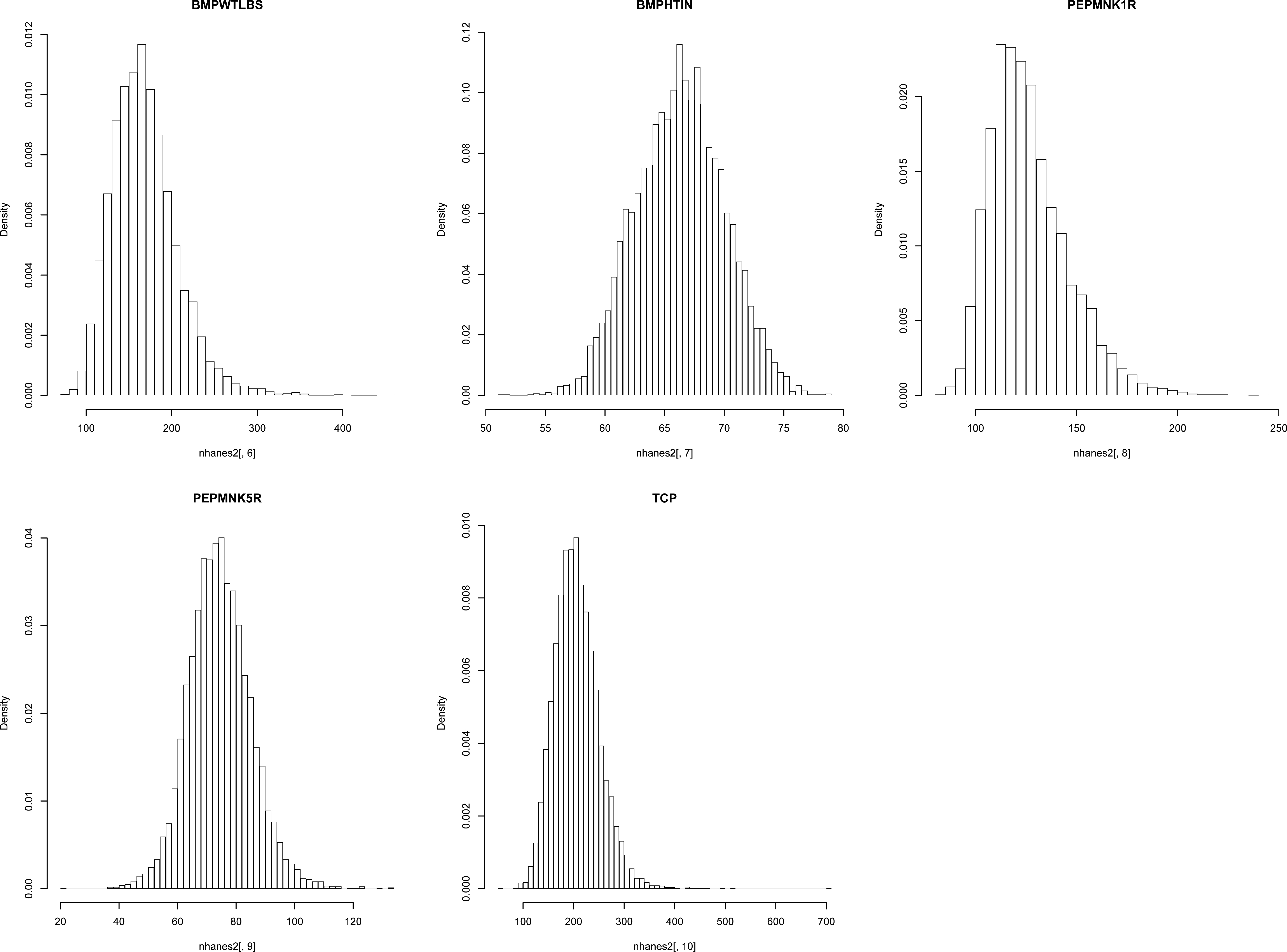

3.2 Simulation setting

In our simulation study, we select five quantitative variables; BMPWTLBS, BMPHTIN, PEPMNK1R, PEPMNK5R, and TCP from the “nhanes3” data set that is available in survey package of the statistical software R. There are 7,927 individuals who do not have any missing on the five variables. We use these as the complete data during our simulation study. Figures 1 and 2 show that three variables BMPWTLBS, PEPMNK1R, and TCP are skewed to the right. Table 2 summarizes the sample variance, skewness and excessive kurtosis of the five variables. We generate missing observations from these three variables at 5% and 15% missing completely at random rates. With 5% and 15% missing rates, the proportions of the complete observations are approximately 85.74% and 61.41%, respectively. For each configuration of the missing rate, we generated 500 incomplete datasets to compare and evaluate the performances of the imputation methods. Figure 3 shows typical missing patterns of the simulated datasets at 5% and 15% missing rates, respectively. For computing the variance estimation in complex survey data, we used survey R package from Complex Surveys: A Guide to Analysis Using R (Lumley, 2010).

Table 2
Sample variance, skewness and excessive kurtosis of the five variables

Variable	Variance	Skewness	Excessive Kurtosis
BMPWTLBS	1477.49	0.9721	2.3613
BMPHTIN	13.59	$-$ 0.0260	$-$ 0.2156
PEPMNK1R	375.12	0.9671	1.3511
PEPMNK5R	114.50	0.2865	0.9507
TCP	1922.61	0.8163	3.2284

Table 3

Average computing time of imputation methods in seconds

Method	kNN	PCA	SVD	PMM	RF	Copula
Time	0.0246	0.425	0.736	4.956	109.588	576.033

Figure 2.

Q-Q plots of the five variables: BMPWTLBS, BMPHTIN, PEPMNK1R, PEPMNK5R, and TCP.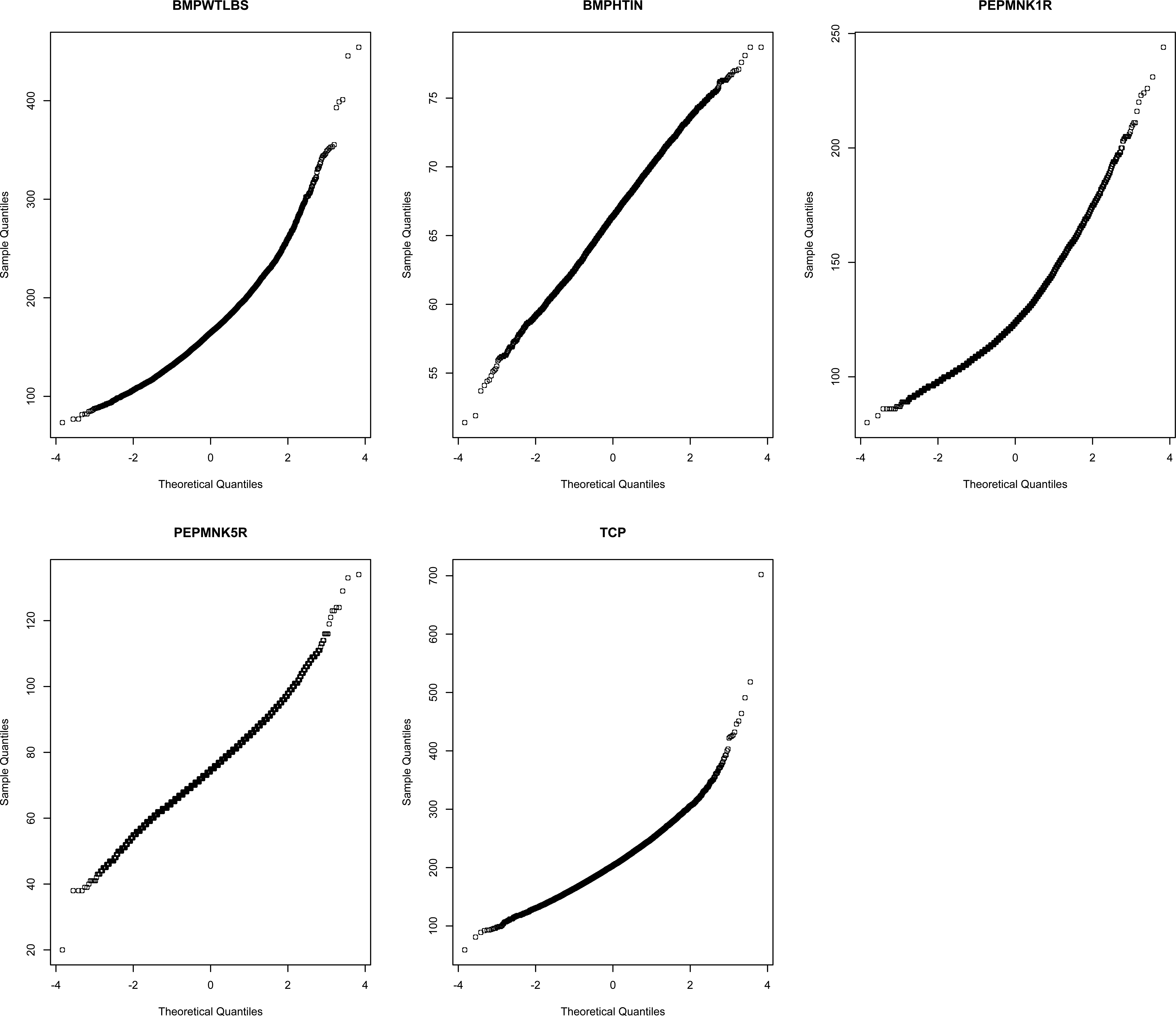

4. Results

We summarize the results of the simulation studies in this section. Dong and Peng (2013) mentioned the proportion of missing data is directly related to the quality of statistical inferences. Yet, there is no established cutoff from the literature regarding an acceptable percentage of missing data in a data set for valid statistical inferences. For example, Schafer (1999) asserted that a missing rate of 5% or less is inconsequential. Bennett (2001) maintained that statistical analysis is likely to be biased when more than 10% of data are missing. Furthermore, the amount of missing data is not the sole criterion by which a researcher assesses the missing data problem. Tabachnick and Fidell (2001) posited that the missing data mechanisms and the missing data patterns have greater impact on research results than does the proportion of missing data.

The illustration of the multivariate imputation models using the NHANES III dataset, which are described by 16 variables classifies people described by a set of attributes as whether smoking influence people or not i.e whether the individual got high blood pressure or not caused by smoking. In this example the covariate variables are showing the health condition of the individuals. Three skewed distributed independent variables were taken to this analysis and these variables describe the status of the individuals in Table 1.

Table 4
Simulation results: Standard errors of the sample mean at 5% missing rate

	Method	SRS	Stratified	Bootstrap	Jackknife	Cluster
BMPWTLBS	Complete	0.7129	0.7128	0.7077	0.7130	1.3687
	Copula	0.7638	0.7636	0.7741	0.7639	1.1882
	RF	0.7044	0.7042	0.6931	0.7044	1.2514
	kNN	0.7150	0.7148	0.7133	0.7150	1.1928
	PCA	0.7008	0.7005	0.7057	0.7007	1.2175
	SVD	0.7151	0.7150	0.7056	0.7153	1.3538
	PMM	0.7145	0.7144	0.7010	0.7146	1.3292
PEPMNK1R	Complete	0.2707	0.2703	0.2616	0.2704	0.0400
	Copula	0.3210	0.3207	0.3105	0.3208	0.2762
	RF	0.2649	0.2644	0.2608	0.2645	0.0828
	kNN	0.2659	0.2654	0.2669	0.2655	0.1384
	PCA	0.2632	0.2627	0.2627	0.2628	0.1325
	SVD	0.2740	0.2736	0.2749	0.2737	0.0677
	PMM	0.2742	0.2738	0.2716	0.2738	0.1085
TCP	Complete	0.6984	0.6981	0.7053	0.6983	1.7878
	Copula	0.8763	0.8760	0.8835	0.8762	0.4353
	RF	0.6867	0.6864	0.6790	0.6866	1.6583
	kNN	0.7427	0.7426	0.7458	0.7429	1.8113
	PCA	0.6817	0.6814	0.6760	0.6816	1.5734
	SVD	0.7031	0.7026	0.7121	0.7028	1.4507
	PMM	0.6995	0.6993	0.6847	0.6995	1.7857

Figure 3.

Missing patterns at 5% (Left) and 15% (Right) missing rates.

We conducted simulation studies using National Health and Nutrition Survey data considering 5% and 15% missing rates. Based on our 500 times resampling simulation study of standard errors of the sample mean in complex survey designs, we can conclude that the principal component analysis (PCA) imputation method appears to outperform other imputation methods overall in Tables 2 and 3. But the copula imputation method shows relatively good performance in clustering sampling design and 5% missing rate where the data are skewed to right because the standard error of each missing data design by using copula Imputation method is smaller than other imputation methods. For TCP variable when 5% missing rate, the distribution of TCP variable is heavily skewed to right. The SE value of the copula imputation is much smaller than the SEs of other imputation methods. In addition, the RF imputation method shows relatively good performance in bootstrap sampling design and 5% missing rate where the data are skewed to right.

The execution time of computing the SEs was related to the size of the dataset especially to the percentage of imputation rate. Especially, under the jackknife method under stratified sampling, it reaches around 300 mins on the largest dataset at the 15% rate of missing values.

The computation time of six imputation methods are quite different. For example, the kNN imputation method is almost immediate whereas the copula imputation method requires 8–10 minutes for completion of imputation. Table 3 summarizes the computing time of each imputation method.

Missing data are a part of almost all research, and there are several alternative ways to overcome the drawbacks they produced. It was previous observed that neutral and well-designed comparison studies in computational sciences are necessary to ensure that previously proposed methods work as expected in various situations and to establish standards and guidelines (Boulesteix et al. 2013).

Table 5

Simulation results: Standard errors of the sample mean at 15% missing rate

	Method	SRS	Stratified	Bootstrap	Jackknife	Cluster
BMPWTLBS	Complete	0.7129	0.7128	0.7077	0.7130	1.3687
	Copula	0.8441	0.8441	0.8431	0.8443	1.1326
	RF	0.6774	0.6773	0.6768	0.6775	1.1786
	kNN	0.6785	0.6785	0.6777	0.6787	1.1675
	PCA	0.6570	0.6570	0.6576	0.6572	1.1464
	SVD	0.6996	0.6996	0.6997	0.6998	1.4898
	PMM	0.7097	0.7096	0.7090	0.7098	1.1809
PEPMNK1R	Complete	0.2707	0.2703	0.2616	0.2704	0.0400
	Copula	0.3624	0.3622	0.3618	0.3623	0.2295
	RF	0.2624	0.2620	0.2613	0.2621	0.0945
	kNN	0.2561	0.2557	0.2558	0.2558	0.0935
	PCA	0.2526	0.2523	0.2521	0.2524	0.0885
	SVD	0.2757	0.2755	0.2758	0.2756	0.0997
	PMM	0.2809	0.2805	0.2807	0.2806	0.1304
TCP	Complete	0.6984	0.6981	0.7053	0.6983	1.7878
	Copula	1.1124	1.1124	1.114	1.1128	1.3041
	RF	0.6557	0.6554	0.6544	0.6556	1.4906
	kNN	0.7011	0.7009	0.7019	0.7011	1.1675
	PCA	0.6436	0.6433	0.6439	0.6435	1.5219
	SVD	0.7300	0.7297	0.7293	0.7299	1.6434
	PMM	0.7096	0.7094	0.7114	0.7096	1.4687

Table 6

RE(%): MSE of the sample mean at 5% missing rate

	Method	SRS	Stratified	Bootstrap	Jackknife	Cluster
BMPWTLBS	Copula	27.90	27.90	29.65	27.91	62.85
	RF	98.48	98.48	104.73	98.48	108.47
	kNN	25.98	25.97	27.60	25.99	59.36
	PCA	99.93	99.93	105.99	99.93	109.30
	SVD	93.86	93.86	99.66	93.86	94.76
	PMM	93.61	93.61	99.39	93.61	107.61
PEPMNK1R	Copula	54.18	54.09	56.75	54.09	2.29
	RF	73.71	73.63	77.32	73.64	4.89
	kNN	69.53	69.44	72.94	69.45	4.00
	PCA	62.89	62.80	65.95	62.81	3.09
	SVD	74.36	74.27	78.02	74.27	5.31
	PMM	70.40	70.31	73.85	70.32	4.23
TCP	Copula	4.62	4.62	4.76	4.62	25.44
	RF	99.12	99.11	101.95	99.11	109.47
	kNN	11.69	11.68	12.04	11.68	48.56
	PCA	97.49	97.48	100.16	97.48	109.24
	SVD	82.66	82.64	85.20	82.65	99.90
	PMM	89.78	89.76	92.51	89.76	109.69

Table 7

RE(%): MSE of the sample mean at 15% missing rate

	Method	SRS	Stratified	Bootstrap	Jackknife	Cluster
BMPWTLBS	Copula	8.26	8.25	7.44	8.26	26.63
	RF	85.52	85.52	72.12	85.54	119.15
	kNN	9.21	9.20	8.29	9.21	28.79
	PCA	98.44	98.43	88.52	98.44	128.15
	SVD	64.73	64.73	58.28	68.74	77.60
	PMM	77.87	77.87	70.22	77.88	113.94
PEPMNK1R	Copula	30.47	30.39	32.67	30.40	0.86
	RF	22.72	22.65	24.36	22.66	0.60
	kNN	25.08	25.02	26.87	25.03	0.67
	PCA	15.55	15.50	16.66	15.51	0.38
	SVD	23.95	23.88	25.64	23.89	0.65
	PMM	23.43	23.37	25.09	23.38	0.61
TCP	Copula	0.79	0.78	0.82	0.79	5.06
	RF	95.48	95.45	100.15	95.46	134.95
	kNN	3.21	3.21	3.36	3.21	18.72
	PCA	84.66	84.62	88.45	84.64	125.64
	SVD	41.72	41.69	43.66	41.70	91.41
	PMM	70.91	70.91	73.91	70.92	128.29

However, only a few studies report an evaluation of existing imputation methods (Brock et al., 2008; Celton et al., 2010; Luengo et al. 2012). In the present study, we performed a neutral comparison of six imputation methods based on four real datasets of various sizes, under an MAR assumption. Validation of imputation results is an important step and we consequently considered two evaluation criteria: standard error (SE) and execution time. While much attention has been paid to the imputation accuracy measured by Root Mean Square Error (RMSE), some studies have examined the effect of imputation on high-level analyses such as unsupervised and supervised classification (Boulesteix et al., 2013; Wang et al., 2006), or the time of execution (Saunders et al., 2006). We found that the sample means by using all six multivariate imputation methods are slightly biased compared with the unbiased sample mean by the complete sample data. To see the magnitude of the gain in efficiency of using the multivariate imputation methods, we compute the percent relative efficiency (RE(%)) of the mean square error (MSE) of the sample mean by using one of six multivariate imputation methods introduced with respect to the MSE of sample mean by the complete sample data as follows

$\textit{RE}(\%)=\frac{\textit{MSE}(\overline{X}_{C})}{\textit{MSE}(\overline{X% }_{I})}\times 100\%,$

where $\textit{MSE}(\overline{X}_{I})$ denotes the MSE of the sample mean by one of six multivariate Imputation methods and $\textit{MSE}(\overline{X}_{c})$ denotes the MSE of the sample mean obtained by complete sample data, and we know $\textit{MSE}(\overline{X})=\textit{Var}(\overline{X})+\textit{Bias}(\overline{% X})^{2}$ . If the value of RE(%) is greater than 100, then the proposed estimator by using one of six multivariate imputation methods is more efficient than the estimator by the complete sample data.

As shown in Table 6 at 5% missing rate, the values of RE(%) for BMPWTLBS are more than 100 for the RF and PCA imputation methods and the most of values of RE(%) for PEPMNK1R variable are more than 100 for the PCA imputation method. We can say that for 5% missing rate, the estimators by the RF and PCA imputation methods are more efficient than the estimator by the complete sample data when the data has high skewness. Similarly, Table 7 at 15% missing rate shows that the values of RE(%) for BMPWTLBS variable are more than 100 for the PCA imputation method, the values of RE(%) for TCP variables are more than 100 for the RF imputation method. We can say that for 15% missing rate and the estimators by the RF and PCA imputation methods are mostly more efficient than the estimator by the complete sample data. Especially, the multivariate imputation methods appears to be efficient in the cluster sampling design when the data has high skewness or excessive kurtosis at the 15% MAR rate.

5. Discussion and conclusions

We compared several multivariate imputation methods for missing data. This work revealed novel insights into the performance of variance estimation of the sample mean by a variety of modern multivariate imputation methods including copula imputation, random forest imputation, and k-nearest neighbors imputation methods in complex designs such as stratified sampling, cluster sampling and replication approach to variance estimation by using jackknife and bootstrap methods in stratified sampling. We conducted simulation studies using National Health and Nutrition Survey data considering 5% and 15% missing rates. Based on our 500 times resampling simulation study of MSE of the sample mean in complex survey designs, the PCA and RF imputation methods appear to outperform other imputation methods when the data has high skewness or excessive kurtosis at the 15% missing rate. In the clustering sampling design, most of the multivariate imputation methods performed well even if the estimators by the multivariate imputation methods have biased estimators. Our findings in this paper suggest that more research is necessary to understand the effects of the multivariate imputation methods in complex survey designs.

References

Arnab

, & Singh

(2006). A new method for estimating variance from data imputed with ratio method of imputation. Statistics & Probability Letters, 76(5), 513-519.

Bennett

D. A.

(2001). How can I deal with missing data in my study? Australian and New Zealand Journal of Public Health, 25(5), 464-469.

Boulesteix

A.-L.

Lauer

, & Eugster

M. J.

(2013). A plea for neutral comparison studies in computational sciences. PloS One, 8(4), e61562.

Breiman

(2001). Random forests. Machine Learning, 45(1), 5-32.

Brock

G. N.

Shaffer

J. R.

Blakesley

R. E.

Lotz

M. J.

, & Tseng

G. C.

(2008). Which missing value imputation method to use in expression profiles: A comparative study and two selection schemes. BMC Bioinformatics, 9(1), 1.

Celton

Malpertuy

Lelandais

, & De Brevern

A. G.

(2010). Comparative analysis of missing value imputation methods to improve clustering and interpretation of microarray experiments. BMC Genomics, 11(1), 1.

De Brevern

A. G.

Hazout

, & Malpertuy

(2004). Influence of microarrays experiments missing values on the stability of gene groups by hierarchical clustering. BMC Bioinformatics, 5(1), 1.

Di Lascio

F. M. L.

, & Giannerini

(2016). CoImp: Copula Based Imputation Method. R package version 0.3-1.

Di Lascio

F. M. L.

Giannerini

, & Reale

(2015). Exploring copulas for the imputation of complex dependent data. Statistical Methods & Applications, 24(1), 159-175.

10.

Dong

, & Peng

C.-Y. J.

(2013). Principled missing data methods for researchers. Springer Plus, 2, 222.

11.

Gabriel

K. R.

, & Zamir

(1979). Lower rank approximation of matrices by least squares with any choice of weights. Technometrics, 21(4), 489-498.

12.

Groves

R. M.

(2004). Survey Errors and Survey Costs, volume 536. John Wiley & Sons.

13.

Groves

R. M.

Presser

, & Dipko

(2004). The role of topic interest in survey participation decisions. Public Opinion Quarterly, 68(1), 2-31.

14.

Groves

R. M.

Singer

, & Corning

(2000). Leverage-saliency theory of survey participation: Description and an illustration. The Public Opinion Quarterly, 64(3), 299-308.

15.

Heitjan

D. F.

, & Basu

(1996). Distinguishing “missing at random” and “missing completely at random”. The American Statistician, 50(3), 207-213.

16.

Hill

(2012). Four techniques for dealing with missing data in criminal justice. In The ASC Annual Meeting, Palmer House Hilton, Chicago, IL.

17.

Horvitz

D. G.

, & Thompson

D. J.

(1952). A generalization of sampling without replacement from a finite universe. Journal of the American statistical Association, 47(260), 663-685.

18.

Hosmer

, & Lemeshow

(2000). Applied logistic regression. New York, ny: A wiley-interscience publication.

19.

Käärik

(2006). Imputation algorithm using copulas. Advances in Methodology and Statistics, 3(1), 109-120.

20.

Käärik

, & Käärik

(2009). Modeling dropouts by conditional distribution, a copula-based approach. Journal of Statistical Planning and Inference, 139(11), 3830-3835.

21.

Kim

J. K.

, & Shao

(2013). Statistical Methods for Handling Incomplete Data. CRC Press.

22.

Kim

J.-M.

, & Anderson

J. E.

(2004). Jackknife variance estimation for two samples after imputation under two-phase sampling. 2004 Proceedings for the American Statistical Association, Section on Survey Research Methods, 3816-3820.

23.

Kim

J.-M.

Sungur

E. A.

, & Heo

T.-Y.

(2007). Calibration approach estimators in stratified sampling. Statistics & Probability Letters, 77(1), 99-103.

24.

Kowarik

, & Templ

(2016). Imputation with the r package vim. Journal of Statistical Software, 74(1), 1-16.

25.

Krzanowski

(1988). Missing value imputation in multivariate data using the singular value decomposition of a matrix. Biometrical Letters, 25(1-2), 31-39.

26.

Little

R. J.

(1988). Missing-data adjustments in large surveys. Journal of Business & Economic Statistics, 6(3), 287-296.

27.

Luengo

García

, & Herrera

(2012). On the choice of the best imputation methods for missing values considering three groups of classification methods. Knowledge and Information Systems, 32(1), 77-108.

28.

Lumley

(2010). Complex surveys: A guide to analysis using R. Hoboken: John Wiley & Sons.

29.

Rieger

Hothorn

, & Strobl

(2010). Random forests with missing values in the covariates. Technical Report.

30.

Rubin

D. B.

(1976). Inference and missing data. Biometrika, 63(3), 581-592.

31.

Rubin

D. B.

(1986). Statistical matching using file concatenation with adjusted weights and multiple imputations. Journal of Business & Economic Statistics, 4(1), 87-94.

32.

Saunders

J. A.

Morrow-Howell

Spitznagel

Doré

Proctor

E. K.

, & Pescarino

(2006). Imputing missing data: A comparison of methods for social work researchers. Social Work Research, 30(1), 19-31.

33.

Schafer

J. L.

(1999). Multiple imputation: A primer. Statistical Methods in Medical Research, 8(1), 3-15.

34.

Schmitt

Mandel

, & Guedj

(2015). A comparison of six methods for missing data imputation. Journal of Biometrics & Biostatistics, 6(1).

35.

Singh

(2003). Advanced Sampling Theory with Applications: How Michael Selected Amy, volume 2. Springer Science & Business Media.

36.

Singh

Sedory

S. A.

Rueda

M. D. M.

Arcos

, & Arnab

(2015). A New Concept for Tuning Design Weights in Survey Sampling: Jackknifing in Theory and Practice. Academic Press.

37.

Stekhoven

D. J.

& Bühlmann

(2012). Missforest – non-parametric missing value imputation for mixed-type data. Bioinformatics, 28(1), 112-118.

38.

Tabachnick

B. G.

Fidell

L. S.

, & Osterlind

S. J.

(2001). Using Multivariate Statistics. Allyn and Bacon Boston.

39.

Tukey

J. W.

(1958). Bias and confidence in not-quite large samples. Annals of Mathematical Statistics, 29(2), 614-614.

40.

Wang

Guo

Zhu

Yang

Wang

, & Rao

(2006). Effects of replacing the unreliable cdna microarray measurements on the disease classification based on gene expression profiles and functional modules. Bioinformatics, 22(23), 2883-2889.

41.

Yeo

Mantel

, & Liu

T-P..

(1999). Bootstrap variance estimation for the national population health survey. In American Statistical Association, Proceedings of the Survey Research Methods Section, 778-783. Citeseer.

Variance estimation by multivariate imputation methods in complex survey designs

Abstract

Keywords

1. Introduction

2. Method

2.1 Modern multivariate imputation methods for missing data

3. Data set and simulation study

3.1 NHANES III data set

Table 1 NHANES III data set

Table 2 Sample variance, skewness and excessive kurtosis of the five variables

Table 4 Simulation results: Standard errors of the sample mean at 5% missing rate

References

Table 1
NHANES III data set

Table 2
Sample variance, skewness and excessive kurtosis of the five variables

Table 4
Simulation results: Standard errors of the sample mean at 5% missing rate