Financial volatility estimation using functional gradient descent algorithm

Abstract

In this paper, we propose a semiparametric method for modeling the volatility in financial time series. The aim is to improve the forecasting capabilities of the most popular parametric volatility models and we also compare our approach to two recent semiparametric models in the literature. Our method is based on the bivariate Bernstein basis polynomials and the functional gradient descent (FGD) algorithm. We evaluate our method through simulated and real datasets. The results demonstrate its good predictive potential for financial volatility.

Keywords

Financial time series volatility functional gradient descent GARCH e-GARCH GJR-GARCH bivariate Bernstein basis polynomials

1. Introduction

Volatility modeling has been one of the most active and extensive research areas in empirical finance and time series economics for both academics and practitioners. It plays a critical role in pricing derivatives, calculating measures of risk, and hedging. It has also sparked an enormous interest and a large number of models have been developed since the seminal works of autoregressive conditional heteroscedasticity (ARCH) by Engle (1982) and generalized autoregressive conditional heteroscedasticity (GARCH) by Bollerslev (1986). ARCH/GARCH models have been very popular in empirical finance and time series economics due to their simple model specification and good interpretability. They have been frequently used in the parametrization of conditional heteroscedasticity in the literature. The GARCH model with order (1, 1), or GARCH(1, 1), is specified as

$\sigma_{t}^{2}=\omega+\alpha X_{t-1}^{2}+\beta\sigma_{t-1}^{2},$ (1)

where $\omega,\alpha$ , and $\beta$ are positive values. This has been used widely and investigated extensively. Gokcan (2000) showed that GARCH(1, 1) outperforms the exponential GARCH model when applied to the monthly stock market returns of seven emerging countries. Hansen and Lunde (2005) compared GARCH(1, 1) with 330 ARCH-type models and found no evidence that it is outperformed by more sophisticated models. Furthermore, GARCH (1, 1) has been used as a benchmark for more complicated model specifications.

Despite the popularity and wide applicability, GARCH models suffer from several weaknesses and drawbacks. Nelson (1991) criticizes GARCH in three aspects: (1) parameters are restricted to be positive at every time point; (2) it fails to accommodate the asymmetry effect (or leverage effect); and (3) measuring the persistence of the shocks on volatility is difficult. To remedy these, Nelson (1991) proposed the exponential GARCH (E-GARCH), which accommodates the drawbacks of GARCH models. The the first-order E-GARCH process, or E-GARCH(1, 1), is specified as

$\log\sigma_{t}^{2}=\omega+g(\varepsilon_{t-1})+\beta[\log(\sigma_{t-1}^{2})],$ (2)

where $g(\varepsilon_{t-1})=\alpha\varepsilon_{t-1}+\gamma(|\varepsilon_{t-1}|-E|% \varepsilon_{t-1}|)$ . For the standard normal random variable $\varepsilon_{t}$ , $E(|\varepsilon_{t}|)=\sqrt{2/\pi}$ and

$E(|\varepsilon_{t}|)=\frac{2\sqrt{v-2}\Gamma(\frac{v+1}{2})}{(v-1)\Gamma(\frac% {v}{2})\sqrt{\pi}}$

for a $t$ -distribution random variable with $v$ degrees of freedom where $\Gamma(\cdot)$ is the gamma function. Unlike GARCH model, the E-GARCH model relaxes the positivity restriction by using the logged conditional variance and responds asymmetrically to positive and negative shocks. However, E-GARCH(1, 1) with normal errors does not adequately characterize the process with high kurtosis and slowly decaying autocorrelations. One can find more details from Malmsten and Terasvirta (2004).

Another popular volatility model that asymmetrically treats both positive and negative shocks on the volatility is the GJR-GARCH model (Glosten et al., 1993). GJR-GARCH(1, 1) model is defined as

$\sigma_{t}^{2}=\omega+\alpha X_{t-1}^{2}+\gamma I_{t-1}X_{t-1}^{2}+\beta\sigma% _{t-1}^{2},$ (3)

where $I_{t}$ is an indicator function taking the values of 1 for $X_{t}\leqslant 0$ and 0 otherwise and $\omega,\alpha,\gamma$ , and $\beta$ are positive values. This model is often called the threshold GARCH (T-GARCH) model in the literature. The main feature of this model is that a negative shock has a larger impact than a positive shock and hence, it captures the leverage effect. Like GARCH model, the GJR-GARCH model captures the volatility clustering. Also, it can be shown that the unconditional distribution presents excess kurtosis even under the Gaussian distribution.

Semiparametric volatility models have gained momentum in the last several years. Linton (2009) and Linton and Yan (2011) examined some advances in semiparametric (and nonparametric) volatility modeling. Ziegelmann (2011) proposed a residual-based semiparametric method to estimate the multivariate volatility. Wang et al. (2012) considered a class of semiparametric GARCH models with additive autoregressive components linked together by a dynamic coefficient. Koo and Linton (2013) have examined the robust estimation on semiparametric multiplicative volatility models under a semi-strong GARCH(1, 1) process with heavy tailed errors. More recently, Liu and Yang (2016) proposed a cubic-spline-based semiparametric GARCH model and demonstrated that it is computationally more efficient than the kernel method. Zhang et al. (2017) used the Box-Cox transformation on the absolute return series and developed an iterative plug-in algorithm to estimate the volatility.

In this paper, we also propose a semiparametric method to model financial volatility where the nonparametric part is constructed from basis functions. As a similar line of research, several attempts have been made to construct a semiparametric volatility model from splines and kernel smoothing. Engle and Rangel (2008) proposed the spline-GARCH model to specify high-frequency return volatility as the low-frequency volatility by an exponential spline basis and the unit GARCH. Audrino and Bühlmann (2009) used B-spline basis functions to approximate the conditional variance function. Wang et al. (2012) examined a semiparametric GARCH model where the parameters are estimated by polynomial spline basis functions. These spline-based models, however, require knot selections and this adds computational complexity to the models. Ruppert (2012), Zhou and Shen (2001), and Spiriti et al. (2013) have examined some ways to select the knots efficiently. Along with the spline-based methods, the kernel smoothing is another approach to estimate the unknown functions. Audrino (2005) proposed ARCH(1) models based on kernel regression in which the estimated volatility is obtained from the local log-likelihood. The procedure requires a kernel function and an optimal bandwidth. Linton and Mammen (2005) investigated a class of semiparametric ARCH( $\infty$ ) models based on kernel smoothing and profile likelihood. A challenge in kernel smoothing is the bandwidth selection as it bears danger of over- and under-smoothing. One can refer to Wand and Jones (1995) for more details. Splines and kernel smoothing are very useful and flexible but they add challenges to the model estimation. Unlike spline- and smoothing-based estimators, the advantage of our approach is the absence of knot and bandwidth selections.

In the current research, we adopt the method of sieve, which was developed by Grenander (1981). The estimator is based on a sequence of bivariate Bernstein basis polynomials and it attempts to improve the estimated parametric model forecast. Bernstein-type estimators have been used by many. Chack et al. (2005); Chang et al. (2005), Chang et al. (2007), and Petrone (1999) examined the nonparametric monotone curve estimation using Bernstein polynomials. More recently, Wang and Ghosh (2012) proposed a method for nonparametric regression based on Berstein polynomials where only assumption is the shape of underlying function. Wang and Ghosh (2013) examined nonparametric model for longitudinal data using Berstein polynomials. Although Bernstein-based estimators and models exist in the literature, it has never been used in financial volatility modeling and the novelty of our work comes from this fact and also from the fact the our method does not require any tuning parameters such as knot and bandwidth.

The paper is organized as follows. Section 2 defines the notations and model. In Section 3, we describe the estimation procedure. Section 4 examines simulated data and Section 5 presents the results using the real data. Lastly, Section 6 concludes.

2. Notations and model formulation

We consider a stochastic process $\{X_{t}:t\in\mathbb{Z}\}$ adapted to filtration $\{\mathcal{F}_{t}:t\in\mathbb{Z}\}$ , where $\mathcal{F}_{t}=\sigma(\{X_{s}:s\leqslant t\})$ and $\sigma(\{X_{s}\})$ is a sigma-field generated by $\{X_{s}\}$ . Let the data generating process (DGP) be

$X_{t}=\mu_{t}+\sigma_{t}\varepsilon_{t},$ (4)

where the innovation $\varepsilon_{t}\sim\text{IID}(0,1)$ for $t=1,...,T$ and $\varepsilon_{t}$ is assumed to be independent of $\{X_{s}:s<t\}$ . Many different specifications, including autoregressive (AR) models, are possible for the mean function $\mu_{t}$ . Kim and Linton (2004) have examined the nonparametric estimation of both $\mu_{t}$ and $\sigma_{t}$ using local instrumental variable. However, we do not pursue the estimation for $\mu_{t}$ in our work. In practice, the stochastic process $\{X_{t}:t\in\mathbb{Z}\}$ resembles return series. For instance, if $Y_{t}$ represents a stock price at a time point $t$ then the return is defined as

$X_{t}=\log(Y_{t})-\log(Y_{t-1}).$

This measures the relative change of the stock price and many financial time series are the return series $X_{t}$ instead of $Y_{t}$ . One can refer to Tsay (2010) for details on some advantages of the return series.

We define

$\sigma_{t}^{2}=f(X_{t-1},\sigma_{t-1}^{2}),$ (5)

where $f$ is a positive-valued function defined on $\mathbb{R}\times\mathbb{R}^{+}$ . The functional form of $f$ is not specified in a nonparametric setting. We note that $\sigma_{t}^{2}$ is the conditional variance $var(X_{t}|\mathcal{F}_{t-1})$ and its square root $\sigma_{t}$ is commonly known as the volatility. Equation (5) defines a general volatility process but this also allows for more complicated dependence of the present volatility from the past. A few people have examined the unknown structure $f(\cdot,\cdot)$ of $\sigma_{t}^{2}$ . Bühlmann and McNeil (2002) examined the nonparametric form of $f$ and provided a regression-based estimation procedure with smoothing. They showed that if $f$ assumes the contraction property

$\textit{sup}_{x\in\mathbb{R}}|f(x,\sigma^{2})-f(x,\tau^{2})|\leqslant D|\sigma% ^{2}-\tau^{2}|$

for some $0<D<1$ , and for all $\sigma^{2},\tau^{2}\in\mathbb{R}^{+}$ and moment conditions $E|\sigma_{t}|^{4}<\infty$ and $E|X_{t-1}|^{4}<\infty$ for all $t$ , then there exists an expansion $h(X_{t-1},X_{t-2},...,X_{t-m})$ for some $m$ that converges to $\sigma_{t}^{2}$ in the $L_{2}$ -sense. More recently, Audrino and Bühlmann (2009) examined the same model with additive expansion of bivariate B-spline basis functions.

The estimation of an unknown function is of interest in many fields but it is often the case that there are too many parameters to be estimated from the data. Also, there might be strong sensitivity of choosing smoothing and/ or tuning parameters. Our approach avoids these two major difficulties. To this end, we first take the logarithmic transformation to avoid the positivity restriction on volatility and then we set the log-squared volatility as

$\displaystyle\log\sigma_{t}^{2}=\log[f(X_{t-1},\sigma_{t-1}^{2})]$ $\displaystyle=g_{0}(X_{t-1},\sigma_{t-1}^{2})+\sum\limits_{j_{1}=0}^{n_{1}}% \sum\limits_{j_{2}=0}^{n_{2}}\beta_{j_{1},j_{2}}B_{j_{1},j_{2}}(X_{t-1},\sigma% ^{2}_{t-1}),$ (6)

where $g_{0}(\cdot,\cdot)$ is a starting parametric log-squared volatility function and $B(\cdot,\cdot)$ is the bivariate Bernstein basis polynomial. Our model specification Eq. (6) can be viewed as a sieve approximation that is guided parametrically by $g_{0}(\cdot,\cdot)$ . Hence, if $\beta_{j_{1},j_{2}}=0$ for all $j_{1},j_{2}$ then the model reduces to a parametric model. In general, we attempt to improve the estimation using the second term

$\sum\limits_{j_{1}=0}^{n_{1}}\sum\limits_{j_{2}=0}^{n_{2}}\beta_{j_{1},j_{2}}B% _{j_{1},j_{2}}(X_{t-1},\sigma^{2}_{t-1}).$

The lagged squared volatility $\sigma^{2}_{t-1}$ is unknown and hence, it is estimated from the previous iteration. The details are given in the next section. A bivariate Bernstein basis polynomial $B(\cdot,\cdot)$ is defined as

$B_{n_{1},n_{2}}(x,\sigma^{2})=\binom{n_{1}}{j_{1}}\binom{n_{2}}{j_{2}}x^{j_{1}% }(1-x)^{n_{1}-j_{1}}(\sigma^{2})^{j_{2}}(1-\sigma^{2})^{n_{2}-j_{2}}=B_{n_{1}}% (x)B_{n_{2}}(\sigma^{2}),$

which is a product of two univariate Bernstein basis polynomials. The Bernstein polynomial is well-known for its use in a constructive proof for the Weierstrass approximation theorem. See Feller (1965) for further details. The arguments of $B_{j_{1},j_{2}}(x,\sigma^{2})$ must lie in the domain [0, 1]. To satisfy this domain restriction, we use the linear transformation defined as

$\frac{y-(y_{(1)}-s)}{(y_{(n)}+s)-(y_{(1)}-s)},$

where $y_{(1)}$ and $y_{(n)}$ are the minimum and maximum order statistics, and $s$ is the sample standard deviation for $y\in\{x,\sigma^{2}\}$ ,

Several attempts have been made to estimate an unknown function using Bernstein polynomials. Babu et al. (2002) applied Bernstein polynomials to estimate the distribution function based on the empirical distribution function smoothing. They established the strong consistency and asymptotic normality of the resulting estimators. Chack et al. (2005) proposed a semi-nonparametric model based on Bernstein polynomials. They proved that their estimation is consistent for true unknown function under some regularity conditions. More recently, Wang and Ghosh (2012) developed a nonparametric regression function estimator with Bernstein polynomials by imposing various shape constraints. Under some mild conditions, they established the strong consistency of their estimator. Wang and Ghosh (2013) also proposed a method to analyze the irregularly observed longitudinal data using a sieve of Bernstein polynomials under a Gaussian process.

3. Estimation procedure

This section describes the estimation procedure. Assuming that the innovations $\{\varepsilon_{t}:t\in\mathbb{Z}\}$ in Eq. (4) are standard normally distributed, the negative log-likelihood function is given by

$\displaystyle-\log\{L(\sigma_{t}^{2};X_{t})\}\propto\sum\limits_{t=2}^{T}\left% [\frac{X_{t}^{2}}{\sigma_{t}^{2}}+\log(\sigma_{t}^{2})\right]$ $\displaystyle=\sum\limits_{t=2}^{T}\left[\frac{X_{t}^{2}}{\exp(g(X_{t-1},% \sigma_{t-1}^{2}))}+g(X_{t-1},\sigma_{t-1}^{2})\right],$ (7)

where $g(X_{t-1},\sigma_{t-1}^{2})=\log\{\sigma_{t}^{2}\}$ . The log-likelihood is conditioned on $X_{1}$ with the starting value $\sigma_{1}^{2}=Var(X_{1}).$ We estimate the parameters by using the functional gradient descent (FGD) algorithm by Friedman (2001). This algorithm considers the function estimation from the perspective of numerical optimization in the function space, rather than parameter space. It requires three things: a differentiable loss function, a base procedure, and an initial starting estimate. We consider the loss function as the likelihood

$L(x,g)=\left[\frac{x^{2}}{\exp(g)}+g\right]$ (8)

and its gradient is then

$U=\frac{\partial L}{\partial g}=\left[1-\frac{x^{2}}{\exp(g)}\right].$

For the base procedure, we use the least squares estimation. As an initial starting estimate, we consider three different parametric models: GARCH(1, 1), EGARCH(1, 1), and GJR-GARCH(1, 1). These models were previously discussed.

We now outline the estimation algorithm. First, let $\{X_{t}:t\in\mathbb{Z}\}$ be defined as in Eq. (4) with $\mu_{t}=0$ and hence, $E(X_{t})=0$ .

Set $m=1$ . Estimate $g_{0}(t)=g_{0}(X_{t-1},\sigma_{t-1}^{2})$ and denote this by $\hat{g}_{0}(t)$ .

Take the loss function $L(x,g)=\left[\frac{x^{2}}{\exp(g)}+g\right]$ and compute the negative gradient from

$U_{t}=-\left[1-\frac{X_{t}^{2}}{\exp(\hat{g}_{m-1}(t))}\right],t=2,...,T.$

Project the negative gradient vector to the space of bivariate Bernstein basis polynomials by the least squares regression

$\hat{S}_{m}=\underset{{\bm{d}}}{\arg\min}\sum\limits_{t=2}^{T}\left\{U_{t}-% \hat{\beta}_{{\bm{d}}}B_{{\bm{d}}}[X_{t-1},\exp(\hat{g}_{m-1}(t)]\right\}^{2},$

where ${\bm{d}}=(d_{1},d_{2})$ is a bivariate index, $\hat{\beta}_{d}$ is the least squares estimated coefficient when regressing $U_{t}$ on $B_{d}[X_{t-1},\exp(\hat{g}_{m-1}(t)]$ .

Perform a linear search for the step length when updating from $\hat{g}_{m}(t)$ to $\hat{g}_{m+1}(t)$ :

$\underset{\rho}{\arg\min}\sum\limits_{t=2}^{T}\left\{L(X_{t},\hat{g}_{m-1}(t)+% \rho B_{d}[X_{t-1},\exp(\hat{g}_{m-1}(t))]\right\}.$

Compute

$\hat{g}_{m}(t)=\hat{g}_{m-1}(t)+\hat{\rho}\hat{\beta}_{\hat{S}_{m}}B_{\hat{S}_% {m}}[X_{t-1},\exp(\hat{g}_{m-1}(t))].$

Increase $m=m+1$ . Repeat Steps 2 and 3.

Step 1 assumes that the nonparametric part is identically equal to zero. Three different initial parametric volatility models are considered.

$\displaystyle\text{GARCH(1, 1): }\hat{g}_{0}(t)=\log\left(\hat{\omega}+\hat{% \alpha}X_{t-1}^{2}+\hat{\beta}\hat{\sigma}_{t-1}^{2}\right)$ $\displaystyle\text{E-GARCH(1, 1): }\hat{g}_{0}(t)=\hat{\omega}+\hat{\alpha}% \epsilon_{t-1}+\hat{\gamma}\left(\epsilon_{t-1}-\sqrt{2/\pi}\right)+\hat{\beta% }\log\hat{\sigma}_{t-1}^{2}$ $\displaystyle\text{GJR-GARCH(1, 1): }\hat{g}_{0}(t)=\log\left(\hat{\omega}+% \hat{\alpha}X_{t-1}^{2}+\hat{\gamma}I_{t-1}X_{t-1}^{2}+\hat{\beta}\hat{\sigma}% _{t-1}^{2},\right)$

As a starting value for $\sigma_{t}^{2}$ , we use the sample variance of the in-sample data. In Step 2, the maximum orders of the bivariate index ${\bm{d}}$ were set to be (5, 5). The optimal index $\hat{d}$ that was chosen in the in-sample period is used in the out-of-sample period. Step 3 performs the one-dimensional line search under the loss function Eq. (8) and gives the $(m+1)$ st estimate of the log-squared volatility. The maximum iteration number was set to be $m=100$ . Our simulation experiments have shown that if our method improves the parametric model then the improvement takes only several iterations or starts at an early stage and the improvement remains constant throughout the latter iterations. Some theoretical justification for the algorithm can be found in Bühlmann and Yu (2003).

4. Simulations

In this section, we test our method through simulations. These simulations will enable us to obtain some feeling for the kinds of processes where the semiparametric procedure can offer better estimates of the unobserved volatility than the parametric modeling. To this end, we consider the following volatility processes.

$\displaystyle\textbf{ A: }f(X_{t-1},X_{t-2},\sigma_{t-1}^{2})=\omega+\alpha_{1% }X_{t-1}^{2}+\alpha_{2}X_{t-2}^{2}+\beta_{1}\sigma_{t-1}^{2}$ $\displaystyle\textbf{ B: }f(X_{t-1},\sigma_{t-1}^{2},\sigma_{t-2}^{2})=\omega+% \alpha_{1}X_{t-1}^{2}+\beta_{1}\sigma_{t-1}^{2}+\beta_{2}\sigma_{t-2}^{2}$ $\displaystyle\textbf{ C: }f(X_{t-1},\sigma_{t-1}^{2})=\omega+\alpha_{1}X_{t-1}% ^{2}+\beta_{1}\sigma_{t-1}^{2}$ $\displaystyle\textbf{ D: }f(X_{t-1},\sigma_{t-1}^{2})=\omega+\alpha_{1}X_{t-1}% ^{2}+\alpha_{2}I_{\left[x\leqslant 0\right]}X_{t-1}^{2}+\beta_{1}\sigma_{t-1}^% {2}$ $\displaystyle\textbf{ E: }f(X_{t-1},\sigma_{t-1}^{2})=\exp\left\{\omega+\alpha% _{1}\varepsilon_{t-1}+\alpha_{2}[|\varepsilon_{t-1}|-\sqrt{2/\pi}]+\beta_{1}% \log(\sigma_{t-1}^{2})\right\}$ $\displaystyle\textbf{ F: }f(X_{t-1},\sigma_{t-1}^{2})=\omega+\left\{1-(1-B)^{% \delta}\right\}X_{t-1}^{2}+\beta_{1}\sigma_{t-1}^{2}$

Some of these processes have stylized facts that can be easily seen in financial datasets. The processes A and B are the GARCH(2, 1) and the GARCH(1, 2), respectively. The process C is the GARCH(1, 1). When $\alpha_{1}+\beta_{1}=1$ it is called the Integrated GARCH (or I-GARCH) model. I-GARCH models have a unit root and the key feature is that the impact of the past squared shocks on the present squared shocks is persistent. Also, the unconditional variance of $X_{t}$ is not defined under I-GARCH(1, 1). Since $\omega>0$ , this process is not covariance stationary but strictly stationary. Several properties of the I-GARCH model have been studied by Nelson (1990). The process D is called the threshold GARCH where switching asymmetry has been built into the ARCH effect. The process E is the E-GARCH. As observed previously, E-GARCH process does not require a parameter restriction and it allows for asymmetric effects between positive and negative returns. The last process is called the fractionally integrated GARCH (FI-GARCH(1, $\delta$ , 1)) model, where $B$ denotes the backshift operator and $\delta\in$ (0, 1). The fractional difference $(1-B)^{\delta}$ can be conveniently expressed in terms of the hypergeometric functions

$\displaystyle(1-B)^{\delta}=F(-\delta,1,1;B)$ $\displaystyle=\sum\limits_{k=0}^{\infty}\Gamma(k-\delta)\Gamma(k+1)^{-1}\Gamma% (-\delta)^{-1}B^{k}$ $\displaystyle=\sum\limits_{k=0}^{\infty}\pi_{k}B^{k},$

where $\Gamma(\cdot)$ is the gamma function. The fractional difference makes the FI-GARCH model to exhibit long memory dynamics. As noted in Rydberg (2000), the long memory characteristic of the return series is one of the main stylized facts from many financial datasets. The differencing parameter $\delta$ controls the long-run behavior and in the ARFIMA model, when $\delta<0.5$ the process is covariance stationary. In ARCH-type models, the stationarity condition depends

Table 1
Performance results were averaged over 50 independent simulations. GARCH-B, E-GARCH-B, and GJR-GARCH-B are the proposed method. Values under each model represents MEAN(STANDARD DEVIATION). * and ** indicate significance at 5% and 1%

Process	$(\omega,\alpha_{1},\alpha_{2},\beta_{1},\beta_{2})$	GOF	GARCH	GARCH-B	DM	E-GARCH	E-GARCH-B	DM	GJR-GARCH	GJR-GARCH-B	DM
A	(0.1, 0.05, 0.7, 0.01, -)	MSE	17.84(82.76)	17.77(82.43)	1.50	24.70(120.29)	23.95(116.26)	1.29	17.79(82.08)	17.71(81.73)	1.46
		HMSE	0.32(0.06)	0.26(0.03)	11.44**	0.44(0.18)	0.36(0.09)	5.57**	0.34(0.07)	0.27(0.04)	11.04**
A	(0.1, 0.7, 0.05, 0.01, -)	MSE	0.07(0.35)	0.07(0.35)	$-$ 0.18	1.40(3.89)	1.36(3.73)	1.29	0.11(0.47)	0.11(0.47)	$-$ 0.27
		HMSE	0.01(0.04)	0.01(0.03)	2.96**	0.08(0.05)	0.08(0.04)	3.59**	0.02(0.04)	0.01(0.03)	2.89**
A	(0.1, 0.01, 0.01, 0.1, -)	MSE	1.50(5.76)	1.52(7.15)	$-$ 0.55	0.00019(0.00015)	0.00018(0.00014)	1.95*	0.00020(0.00025)	0.00018(0.00024)	3.67**
		HMSE	1.14(4.17)	1.124(4.90)	0.38	0.020(0.028)	0.017(0.019)	2.77**	0.010(0.011)	0.0093(0.011)	4.16**
B	(0.1, 0.25, - , 0.03, 0.01)	MSE	0.001(0.001)	0.001(0.001)	3.63**	5.48(28.98)	5.47(28.98)	1.35	0.002(0.001)	0.001(0.001)	3.24**
		HMSE	0.06(0.07)	0.05(0.06)	4.02**	4.00(8.00)	3.00(8.00)	4.03**	0.09(0.10)	0.08(0.09)	3.90**
B	(0.1, 0.05, - , 0.1, 0.05)	MSE	1.07(0.30)	0.98(0.26)	3.12**	1.92(1.20)	1.77(1.17)	5.94**	5.14(7.41)	3.69(4.60)	2.69**
		HMSE	7.04(2.26)	6.13(1.31)	3.62**	13.80(10.11)	11.41(8.43)	6.64**	56.35(133.00)	26.17(33.40)	2.06**
B	(0.1, 0.05, - , 0.05, 0.1)	MSE	1.04(0.26)	1.00(0.28)	2.02**	2.25(0.18)	2.04(0.14)	2.83**	3.74(0.41)	3.234(2.92)	2.94**
		HMSE	6.72(1.64)	6.16(1.34)	3.17**	1.68(1.84)	0.013(0.010)	3.29**	0.049(0.12)	0.027(0.045)	2.10**
C	(0.1, 0.55, - , 0.45, -)	MSE	4.99(18.58)	4.88(18.13)	1.69	385.59(1031.61)	376.52(1006.35)	1.79	11.67(43.27)	11.45(42.35)	1.69
		HMSE	0.021(0.044)	0.019(0.043)	4.01**	0.076(0.046)	0.068(0.036)	2.89**	0.024(0.043)	0.022(0.042)	4.10**
C	(0.1, 0.90, - , 0.10, -)	MSE	4.27(13.11)	4.03(12.25)	2.02**	2.59(12.13)	2.59(12.13)	1.53	7.21(19.38)	6.96(18.58)	2.10**
		HMSE	0.0087(0.0070)	0.0069(0.0053)	4.28**	0.12(0.14)	0.11(0.14)	4.37**	0.0107(0.0074)	0.0087(0.0059)	4.54**
C	(0.1, 0.30, - , 0.70, -)	MSE	14.60(43.06)	13.79(40.50)	2.23**	447.50(1149.59)	395.37(1089.15)	2.52**	18.04(47.53)	15.08(37.61)	2.06**
		HMSE	0.0093(0.010)	0.0080(0.010)	3.01**	0.040(0.018)	0.036(0.012)	3.33**	0.012(0.011)	0.0098(0.010)	2.83**
$C^{\textit{SP}500}$	(0.00022, 0.068, - , 0.92, -)	MSE	1.024(4.01)	0.75(2.76)	1.46	3.01(11.29)	2.21(7.47)	1.47	1.12(4.16)	0.85(2.86)	1.48
		HMSE	0.87(1.44)	0.80(1.32)	2.87**	2.35(4.33)	1.98(2.94)	1.85	1.12(1.46)	1.00(1.29)	2.80**
$C^{\textit{TBond}}$	(0, 0.015, - , 0.97, -)	MSE	1.73(1.31)	1.52(1.32)	4.26**	3.40(3.54)	3.28(3.04)	5.35**	5.66(7.30)	4.70(6.15)	3.41**
		HMSE	0.85(0.67)	0.71(0.66)	4.47**	1.85(1.52)	1.37(1.12)	4.81**	2.23(2.23)	1.80(1.98)	6.13**
D	(0.02, 0.10, 0.30 , 0.50, -)	MSE	0.0010(0.00061)	0.0010(0.0006)	3.79**	0.00070(0.0011)	0.00073(0.0011)	4.06**	0.00022(0.00023)	0.0002(0.0002)	4.16**
		HMSE	0.054(0.059)	0.050(0.053)	4.57**	0.024(0.019)	0.023(0.019)	3.86**	0.012(0.018)	0.010(0.018)	5.01**
D	(0.02, 0.10, 0.50 , 0.10, -)	MSE	0.039(0.015)	0.039(0.015)	4.14**	0.019(0.011)	0.019(0.010)	4.11**	0.0048(0.0043)	0.0045(0.0039)	2.97**
		HMSE	6.21(1.06)	6.04(0.95)	3.81**	2.79(0.81)	2.71(0.83)	3.50**	1.49(1.87)	1.40(1.84)	4.57**
D	(0.02, 0.50, 0.30 , 0.10, -)	MSE	0.0088(0.035)	0.0083(0.033)	1.50	0.075(0.34)	0.072(0.32)	1.29**	0.0070(0.031)	0.0068(0.031)	1.17
		HMSE	0.023(0.011)	0.020(0.007)	3.59**	0.10(0.13)	0.087(0.097)	2.58**	0.013(0.010)	0.010(0.0084)	3.66**
$D^{\textit{SP}500}$	(0.00026, 0.015, 0.091 , 0.93, -)	MSE	0.00052(0.0029)	0.00044(0.0024)	1.14	0.0029(0.019)	0.0016(0.010)	1.02	0.00010(0.00047)	0.00010 (0.00048)	0.94
		HMSE	0.044(0.016)	0.039(0.012)	3.71**	0.056(0.14)	0.038(0.059)	1.44	0.014(0.013)	0.013(0.013)	3.96**
$D^{\textit{TBond}}$	(0.00, 0.01, 0.008 , 0.97, -)	MSE	8.93(36.00)	7.46(35.85)	2.27**	0.032(0.13)	0.029(0.12)	1.86	5.70(30.05)	5.89(30.03)	3.031**
		HMSE	1.20(0.11)	1.10(0.15)	4.80**	0.66(0.31)	0.60(0.26)	2.77**	1.18(0.14)	1.11(0.17)	3.33**
E	(0.1, 0.20, 0.10 , 0.05, -)	MSE	0.075(0.0056)	0.073(0.0058)	3.79**	0.022(0.027)	0.021(0.027)	3.29**	0.11(0.10)	0.098(0.085)	2.69**
		HMSE	0.058(0.0047)	0.053(0.0045)	5.68**	0.015(0.019)	0.012(0.017)	4.45**	0.12(0.27)	0.073(0.068)	1.76
E	(0.1, 0.05, 0.10 , 0.20, -)	MSE	0.012(0.0032)	0.012(0.0034)	1.79	0.66(3.85)	0.47(2.73)	1.21	0.039(0.051)	0.031(0.033)	2.89**
		HMSE	0.0089(0.0017)	0.0084(0.0017)	3.35**	0.023(0.081)	0.020(0.071)	2.37**	0.083(0.27)	0.035(0.072)	1.72
E	(0.1, 0.05, 0.05 , 0.10, -)	MSE	0.0076(0.0032)	0.0072(0.0027)	1.96*	0.28(1.82)	0.24(1.56)	1.05	0.038(0.071)	0.027(0.032)	1.89
		HMSE	0.0060(0.0027)	0.0054(0.0018)	2.50**	0.023(0.051)	0.020(0.048)	4.43**	0.035(0.071)	0.022(0.034)	2.16**
$E^{\textit{SP}500}$	(-0.063, -0.076, 0.12 , 0.98, -)	MSE	0.00022(0.00016)	0.00021(0.00016)	3.55**	0.000077(0.000086)	0.000067(0.000071)	3.51**	0.00011(0.00016)	0.000112(0.00015)	3.13**
		HMSE	0.057(0.022)	0.051(0.017)	3.94**	0.022(0.029)	0.018(0.021)	2.72**	0.025(0.021)	0.022(0.015)	2.53**
$E^{\textit{TBond}}$	(-0.052, 0.0005, 0.04 , 0.98, -)	MSE	8.93(36.00)	7.46(35.85)	2.27**	0.032(0.13)	0.029(0.12)	1.86	5.99(30.47)	5.89(30.29)	3.03**
		HMSE	1.20(0.11)	1.10(0.15)	4.80**	0.66(0.31)	0.60(0.26)	2.77**	1.18(0.14)	1.11(0.17)	3.33**
F	( $\delta=$ 0.1, $\omega=$ 0.25, $\beta=$ 0.05)	MSE	0.0049(0.0029)	0.0046(0.0027)	3.74**	0.091(0.61)	0.055(0.35)	1.01	0.011(0.016)	0.010(0.015)	2.82**
		HMSE	0.023(0.017)	0.019(0.014)	4.12**	0.033(0.070)	0.026(0.047)	2.11**	0.20(1.012)	0.084(0.34)	1.188
F	( $\delta=$ 0.25, $\omega=$ 0.25, $\beta=$ 0.05)	MSE	0.14(0.10)	0.13(0.10)	3.75**	0.18(0.17)	0.17(0.15)	3.32**	0.14(0.11)	0.14(0.11)	3.90**
		HMSE	0.058(0.012)	0.053(0.0079)	4.61**	0.082(0.030)	0.073(0.021)	4.84**	0.062(0.017)	0.056(0.012)	5.20**
F	( $\delta=$ 0.25, $\omega=$ 0.05, $\beta=$ 0.25)	MSE	0.18(0.31)	0.17(0.27)	1.49	0.35(0.76)	0.28(0.55)	1.94	0.19(0.32)	0.17(0.28)	1.51
		HMSE	0.068(0.032)	0.061(0.030)	4.51**	0.098(0.056)	0.083(0.033)	3.15**	0.072(0.032)	0.064(0.030)	4.55**

on the cumulated coefficients from the MA representation. The reader is referred to Baillie et al. (1996) for more details.

To study the sensitivity of our method, we choose a set of different parameters for each process. We generate 2500 observations from each process and we use the first 500 observations as a burn-in period, the next 1000 as the in-sample period to estimate the model, and the last 1000 as the out-of-sample testing period. To assess the accuracy of the volatility estimates, we calculate the goodness-of-fit measures defined by

$\textit{MSE}=\frac{1}{T}\sum\limits_{t=T+1}^{2T}\left(\hat{\sigma}_{t}^{2}-% \sigma_{t}^{2}\right)^{2},$ (9)

and

$\textit{HMSE}=\frac{1}{T}\sum\limits_{t=T+1}^{2T}\left(\hat{\sigma}_{t}^{2}/% \sigma_{t}^{2}-1\right)^{2},$ (10)

where $\hat{\sigma}_{t}^{2}$ is the estimated squared volatility, $\sigma_{t}^{2}$ is the true squared volatility, and $T=1000$ . The parameter estimates in $\hat{\sigma}_{t}^{2}$ are obtained from the in-sample period and both MSE and HMSE are computed from the out-of-sample.

Table 2

Summary statistics for the datasets

Data	Min.	1st Qu.	Median	Mean	3rd Qu.	Max.
SP500	$-$ 1.319	$-$ 0.077	0.007	0.004	0.089	1.288
T-Bond	$-$ 0.425	$-$ 0.043	0.004	0.002	0.053	0.316

Figure 1.

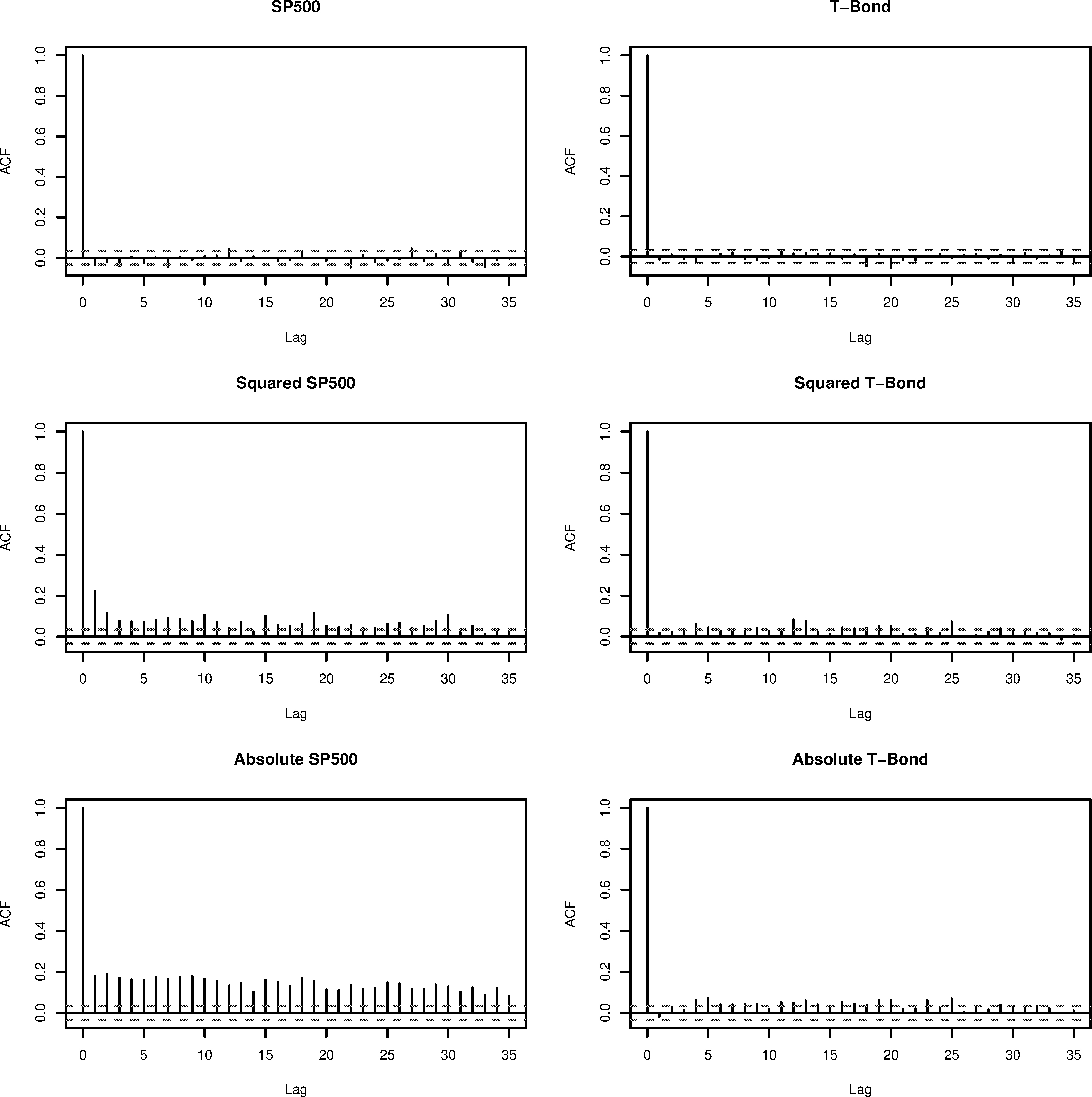
Sample autocorrelation function of raw, squared, and absolute data for both SP 500 and US Treasury bond.

Table 3

Performance results for real-data examples

		In-sample errors		Out-of-sample errors
Data	Model	MSE	HMSE	MSE	HMSE
SP500	GARCH(1,1)	0.0039	4.9040	0.0061	3.3834
	GARCH-B	0.0036(16)	2.0593(16)	0.0060(4)	2.7476(101)
	BC-GARCH	0.0040	10.6902	0.0012	4.1423
	E-GARCH(1,1)	0.0038	4.6974	0.0057	2.9175
	E-GARCH-B	0.0035(101)	2.2462(101)	0.0055(101)	1.5913 (101)
	BC-GARCH	0.0041	26.1766	0.0022	1.9141
	GJR-GARCH(1,1)	0.0038	4.7393	0.0058	3.1304
	GJR-GARCH-B	0.0036(61)	2.2324(13)	0.0056(31)	2.1830(12)
	BC-GARCH	0.0040	9.3691	0.0022	2.1164
	Spline-GARCH	0.0023	7.5829	0.0081	11.0376
T-Bond	GARCH(1,1)	0.0002	3.2053	0.0002	3.2584
	GARCH-B	0.0001(47)	2.5974(13)	0.0002(56)	1.5011(29)
	BC-GARCH	0.0057	1.6196	0.0028	0.8102
	E-GARCH(1,1)	0.0001	3.2287	0.0002	3.0369
	E-GARCH-B	0.0001(101)	2.7017(7)	0.0002(101)	1.5013(101)
	BC-GARCH	0.0173	0.9813	0.0160	0.8437
	GJR-GARCH(1,1)	0.0001	3.2375	0.0002	3.2770
	GJR-GARCH-B	0.0001(60)	2.3581(21)	0.0002(62)	1.5527(26)
	BC-GARCH	0.0401	0.9349	0.0433	0.8850
	Spline-GARCH	0.0025	51.3585	0.0001	2.5503

To test for forecasting accuracy, we perform the Diebold and Mariano (DM) test proposed by Diebold and Mariano (1995). The underlying hypotheses associated with this test are

$H_{0}:E\left(z_{t}^{[1]}\right)=E\left(z_{t}^{[2]}\right)\text{ vs. }H_{1}:E% \left(z_{t}^{[1]}\right)\neq E\left(z_{t}^{[2]}\right),$

where $z_{t}$ is the deviance at time $t$ in Eqs (9) and (10) from models [1] and [2]. In our simulations and real data examples, [1] denotes the parametric model and [2] denotes our semiparametric model. Hence, the null hypothesis indicates the “equal accuracy” between the two models. In a large sample, the DM statistic

$DM=\frac{\sqrt{T-p}(\bar{z}-\mu_{z})}{2\pi f_{z}(0)}\sim N(0,1),$

where $\bar{z}=\frac{1}{T-p}\sum\nolimits_{t=p+1}^{T}\left(z_{t}^{[1]}-z_{t}^{[2]}\right)$ , $f_{z}(0)=\frac{1}{2\pi}\sum\nolimits_{\tau=-\infty}^{\infty}\gamma_{z}(\tau)$ is the spectral density of the loss differential at frequency 0, and $\gamma_{z}(\tau)=E[(z_{t}-\mu)(z_{t-\tau}-\mu)]$ is the autocovariance function at $\tau$ . Hence, a positive value of DM indicates that the average expected deviance is higher for model [1] than that of model [2] and a negative value indicates the lower expected deviance.

We report the simulation results in Table 1. Each value in the table represents the average goodness-of-fit measure from 50 independent simulations and the values in the parentheses are the standard deviations. The models GARCH-B, E-GARCH-B, and GJR-GARCH-B are the semiparametric models that attempt to improve the corresponding parametric models. The values under DM are the test statistic values from the DM test. Again, the null hypothesis associated with this test statistics, for GARCH vs. GARCH-B under MSE as an example, is $E(z_{t}^{\textit{[GARCH]}})=E(z_{t}^{\textit{[GARCH-B]}})$ , where $z_{t}$ is the $t$ -th deviance under MSE. Except for two cases under Process A, all the values of DM are positive. More importantly, the results show that the majority of tests are significant, which indicate significantly better performance of the semiparametric models over the parametric ones. The processes with superscripts SP500 and T-Bond indicate that the coefficients are chosen from the estimated parametric models using the SP500 and T-Bond datasets. In many cases, the semiparametric models have significantly better predictive potential than the parametric models.

Table 4

DM test based on (out-of-sample) squared errors for the optimal iteration number. DM test statistics values are shown. A negative (positive) value indicate better predictive accuracy for the row (column). * and ** indicate significance at 5% and 1%

Data	Model	GARCH(1, 1)	GARCH-B	Spline-GARCH	BC-GARCH
SP500	GARCH(1, 1)	–	$2.45^{*}$	$-$ 1.94	$-$ 1.82
	GARCH-B	$-$ 2.45 ${}^{*}$	–	$-$ 2.16 ${}^{*}$	$-$ 2.03
	Spline-GARCH	1.94	2.16	–	6.43 ${}^{**}$
	BC-GARCH	1.82	2.03	$-$ 6.43 ${}^{**}$	–
	Model	E-GARCH(1, 1)	GARCH-B	Spline-GARCH	BC-GARCH
	E-GARCH(1, 1)	–	2.88 ${}^{**}$	$-$ 2.13 ${}^{*}$	$-$ 2.61 ${}^{**}$
	GARCH-B	$-$ 2.88 ${}^{**}$	–	$-$ 2.48	$-$ 2.87 ${}^{**}$
	Spline-GARCH	2.13 ${}^{*}$	2.48	–	6.37 ${}^{**}$
	BC-GARCH	2.61 ${}^{**}$	2.87 ${}^{**}$	$-$ 6.37 ${}^{**}$	–
	Model	GJR-GARCH(1, 1)	GARCH-B	Spline-GARCH	BC-GARCH
	GJR-GARCH(1, 1)	–	3.65 ${}^{**}$	$-$ 2.17 ${}^{*}$	$-$ 2.12 ${}^{*}$
	GARCH-B	$-$ 3.65 ${}^{**}$	–	$-$ 2.53 ${}^{**}$	$-$ 2.48 ${}^{**}$
	Spline-GARCH	2.17 ${}^{*}$	2.53 ${}^{**}$	–	6.03 ${}^{**}$
	BC-GARCH	2.12 ${}^{*}$	2.48 ${}^{*}$	$-$ 6.03 ${}^{**}$	–
Data	Model	GARCH(1, 1)	GARCH-B	Spline-GARCH	BC-GARCH
T-Bond	GARCH(1, 1)	–	5.41 ${}^{**}$	$-$ 3.61 ${}^{**}$	$-$ 61.93 ${}^{**}$
	GARCH-B	$-$ 5.41 ${}^{**}$	–	$-$ 5.98 ${}^{**}$	$-$ 66.02 ${}^{**}$
	Spline-GARCH	3.61 ${}^{**}$	5.98 ${}^{**}$	–	$-$ 63.06 ${}^{**}$
	BC-GARCH	61.93 ${}^{**}$	66.02 ${}^{**}$	63.06 ${}^{**}$	–
	Model	E-GARCH(1, 1)	GARCH-B	Spline-GARCH	BC-GARCH
	E-GARCH(1, 1)	–	3.49 ${}^{**}$	$-$ 3.88 ${}^{**}$	$-$ 119.62 ${}^{**}$
	GARCH-B	$-$ 3.49 ${}^{**}$	–	$-$ 4.06 ${}^{**}$	$-$ 121.57 ${}^{**}$
	Spline-GARCH	3.88 ${}^{**}$	4.06 ${}^{**}$	–	$-$ 119.94 ${}^{**}$
	BC-GARCH	119.62 ${}^{**}$	121.57 ${}^{**}$	119.94 ${}^{**}$	–
	Model	GJR-GARCH(1, 1)	GARCH-B	Spline-GARCH	BC-GARCH
	GJR-GARCH(1, 1)	–	5.40 ${}^{**}$	3.51 ${}^{**}$	$-$ 108.11 ${}^{**}$
	GARCH-B	$-$ 5.40 ${}^{**}$	–	$-$ 5.99 ${}^{**}$	$-$ 108.38 ${}^{**}$
	Spline-GARCH	3.51 ${}^{**}$	5.99 ${}^{**}$	–	$-$ 108.17 ${}^{**}$
	BC-GARCH	108.11 ${}^{**}$	108.38 ${}^{**}$	108.17 ${}^{**}$	–

Table 5

DM test based on (out-of-sample) heteroskadastic squared errors for the optimal iteration number. DM test statistics values are shown. A negative (positive) value indicate better predictive accuracy for the row (column). * and ** indicate significance at 5% and 1%

Data	Model	GARCH(1, 1)	GARCH-B	Spline-GARCH	BC-GARCH
SP500	GARCH(1, 1)	–	4.39 ${}^{**}$	$-$ 1.02	$-$ 2.74 ${}^{**}$
	GARCH-B	$-$ 4.39 ${}^{**}$	–	$-$ 1.12	$-$ 2.89 ${}^{**}$
	Spline-GARCH	1.02	1.12	–	2.38 ${}^{*}$
	BC-GARCH	2.74 ${}^{**}$	2.89 ${}^{**}$	$-$ 2.38 ${}^{*}$	–
	Model	E-GARCH(1, 1)	GARCH-B	Spline-GARCH	BC-GARCH
	E-GARCH(1, 1)	–	5.09 ${}^{**}$	$-$ 1.08	$-$ 2.89 ${}^{**}$
	GARCH-B	$-$ 5.09 ${}^{**}$	–	$-$ 1.28	$-$ 2.98 ${}^{**}$
	Spline-GARCH	1.08	1.28	–	2.14 ${}^{*}$
	BC-GARCH	2.89 ${}^{**}$	2.98 ${}^{**}$	$-$ 2.14 ${}^{*}$	–
	Model	GJR-GARCH(1, 1)	GARCH-B	Spline-GARCH	BC-GARCH
	GJR-GARCH(1, 1)	–	4.49 ${}^{**}$	$-$ 1.06	$-$ 3.00 ${}^{**}$
	GARCH-B	$-$ 4.49 ${}^{**}$	–	$-$ 1.21	$-$ 3.24 ${}^{**}$
	Spline-GARCH	1.06	1.21	–	2.35 ${}^{*}$
	BC-GARCH	3.00 ${}^{**}$	3.24 ${}^{**}$	$-$ 2.35 ${}^{*}$	–
Data	Model	GARCH(1, 1)	GARCH-B	Spline-GARCH	BC-GARCH
T-Bond	GARCH(1, 1)	–	5.112 ${}^{**}$	0.26	3.52
	GARCH-B	$-$ 5.11 ${}^{**}$	–	$-$ 1.37	2.80 ${}^{**}$
	Spline-GARCH	$-$ 0.26	1.37	–	1.76
	BC-GARCH	$-$ 3.52 ${}^{**}$	$-$ 2.80 ${}^{**}$	$-$ 1.76	–
	Model	E-GARCH(1, 1)	GARCH-B	Spline-GARCH	BC-GARCH
	E-GARCH(1, 1)	–	5.05 ${}^{**}$	0.03	3.75 ${}^{**}$
	GARCH-B	$-$ 5.05 ${}^{**}$	–	$-$ 1.37	2.14 ${}^{*}$
	Spline-GARCH	$-$ 0.03	1.37	–	1.66
	BC-GARCH	$-$ 3.75 ${}^{**}$	$-$ 2.14 ${}^{*}$	$-$ 1.66	–
	Model	GJR-GARCH(1, 1)	GARCH-B	Spline-GARCH	BC-GARCH
	GJR-GARCH(1, 1)	–	5.27 ${}^{**}$	0.32	3.70 ${}^{**}$
	GARCH-B	$-$ 5.27 ${}^{**}$	–	$-$ 1.32	2.23 ${}^{*}$
	Spline-GARCH	$-$ 0.32	1.32	–	1.63
	BC-GARCH	$-$ 3.70 ${}^{**}$	$-$ 2.23 ${}^{*}$	$-$ 1.63	–

5. Real data examples

As examples with real data, we consider the US Standard and Poor’s 500 (SP500) index and 30-year US Treasury bonds (T-Bond) between January 1990 and October 2003. Both datasets consist of 3376 daily log-returns. We use the first 70% of dataset as an in-sample estimation period and the remaining 30% as an out-of-sample test data. These datasets can be obtained from blackwellpublishing.com/rss. Along with the daily return series, high frequency observations are available to create realized volatility, which may be used as a proxy for the unknown underlying true volatility. We compute the same performance statistics Eqs (9) and (10) substituting the true underlying volatility with the realized volatility. Realized volatility is the sum of finely-sampled squared return realizations over a fixed time interval. In a frictionless market, the usual assumption is that the realized volatility attains the consistent estimate from the quadratic return series as they are sampled at a high frequency. The reader is referred to McAleer and Medeiros (2008) for more details and explanations. The summary statistics for the raw data are given in Table 2. Figure 1 shows the sample autocorrelation function (ACF) of the raw, squared and absolute series. Linear time dependence is clearly indicated through higher moments in SP500. Although minimal, the time dependence can also seen in the T-Bond dataset.

Figure 2.

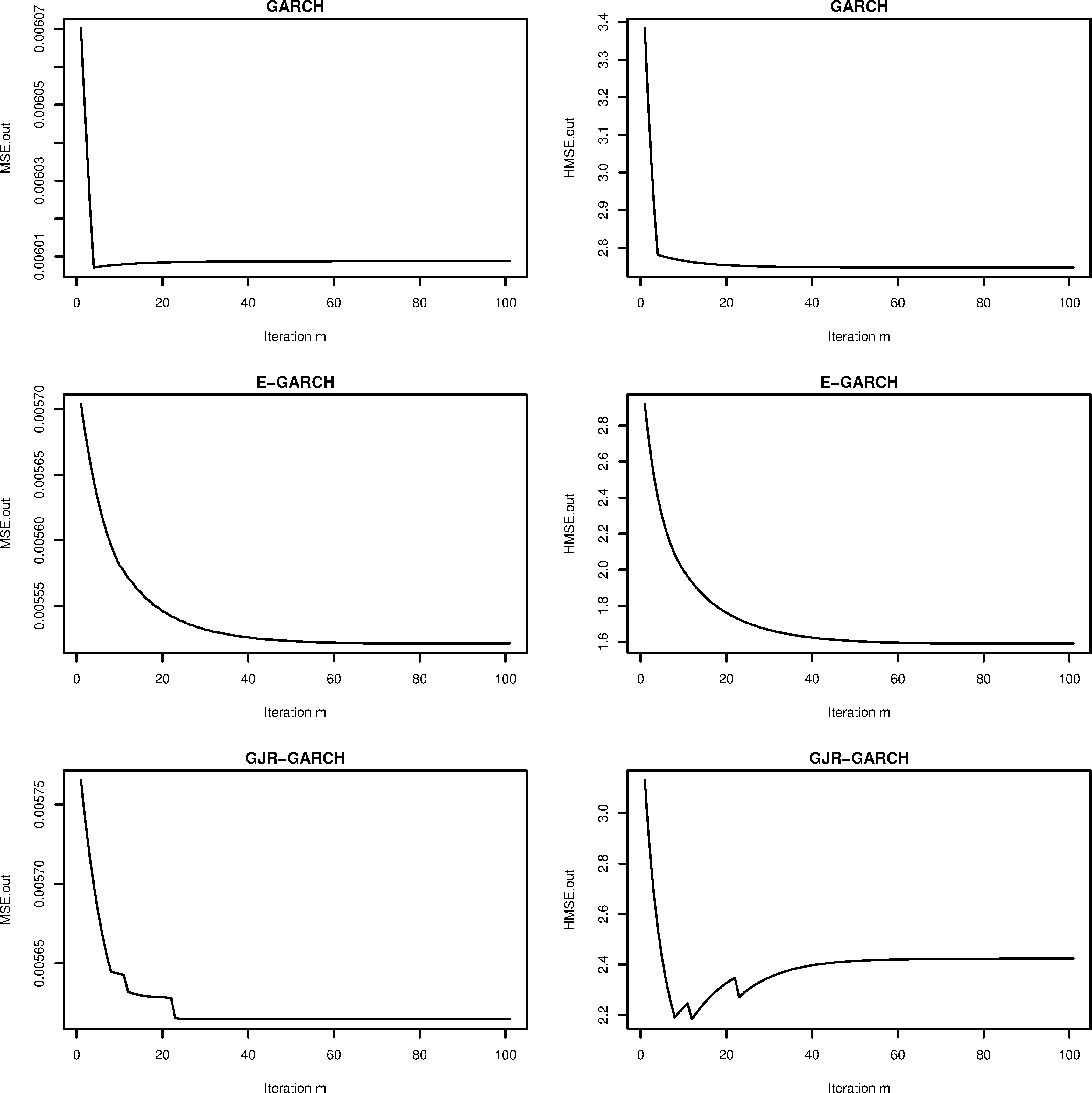
Performance measures are shown by iteration number for SP500.

There is a growing body of literature on semiparametric volatility modeling. To compare our method with the current semiparametric volatility models, we examine two recent semiparametric models that were proposed by Liu and Yang (2016) and Zhang et al. (2017). Liu and Yang (2016) used a cubic spline to model semiparametric GARCH and Zhang et al. (2017)’s model is based on the Box-Cox transformation on the absolute return series. We denote their models as Spline-GARCH and BC-GARCH, respectively. Table 3 gives the results based on the performance measures for both in-sample and out-of-sample periods although the in-sample errors may not be of interest in practice. Analogous to simulations, our method is denoted as GARCH-B, E-GARCH-B, and GJR-GARCH-B. The value in parenthesis is the iteration number when the error measure was minimum. Examining the out-of-sample, the results show that Spline-GARCH performs well under MSE but it poorly performs under HMSE. BC-GARCH performs better than GARCH-B under HMSE but it performs worse under MSE for T-Bond dataset. Hence, there seems to be no consistent comparison among the semiparametric models and further investigation may be needed.

Figure 3.

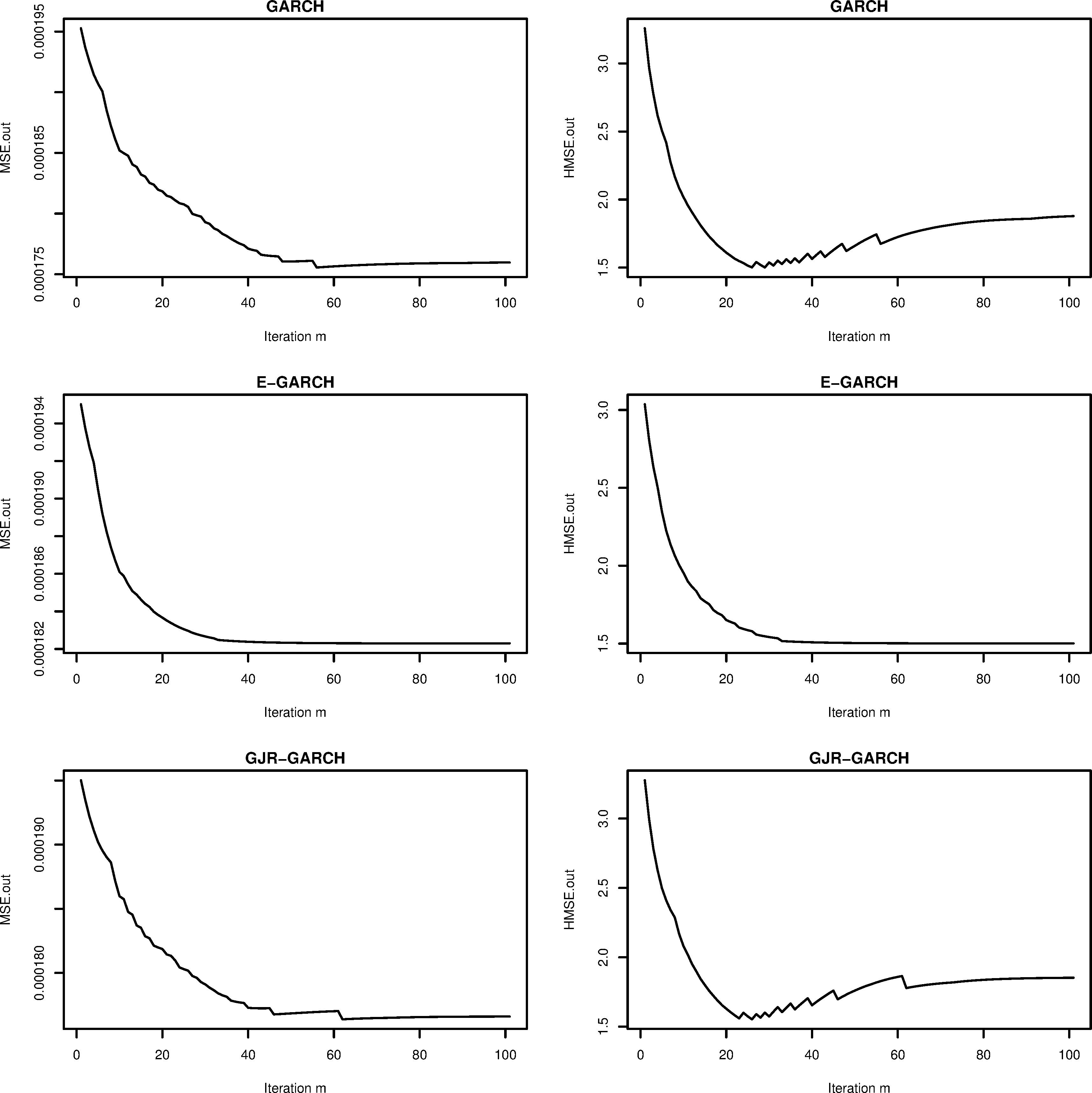
Performance measures are shown by iteration number for T-Bond.

The estimated parametric models for SP500 are

$\displaystyle\text{GARCH(1, 1): }\hat{\sigma}_{t}^{2}=0.00022+0.068X_{t-1}^{2}% +0.92\hat{\sigma}_{t-1}^{2},$ $\displaystyle\text{E-GARCH(1, 1): }\log(\hat{\sigma}_{t}^{2})=-0.063-0.07591% \hat{\epsilon}_{t-1}+0.12(\hat{\epsilon}_{t-1}-\sqrt{2/\pi})+0.98\log(\hat{% \sigma}_{t-1}^{2}),$

and

$\displaystyle\text{GJR-GARCH(1, 1): }\hat{\sigma}_{t}^{2}=0.00026+0.015X_{t-1}% ^{2}+0.091I_{t-1}X_{t-1}^{2}+0.93\hat{\sigma}_{t-1}^{2}.$

Also, the estimated parametric models for T-Bond are

$\displaystyle\text{GARCH(1, 1): }\hat{\sigma}_{t}^{2}=0.000068+0.015X_{t-1}^{2% }+0.97\hat{\sigma}_{t-1}^{2},$ $\displaystyle\text{E-GARCH(1, 1): }\log(\hat{\sigma}_{t}^{2})=-0.052-0.00047% \hat{\epsilon}_{t-1}+0.037(\hat{\epsilon}_{t-1}-\sqrt{2/\pi})+0.98\log(\hat{% \sigma}_{t-1}^{2}),$

and

$\displaystyle\text{GJR-GARCH(1, 1): }\hat{\sigma}_{t}^{2}=0.000084+0.010X_{t-1% }^{2}+0.0080I_{t-1}X_{t-1}^{2}+0.97\hat{\sigma}_{t-1}^{2}.$

The estimates from these models are used in the simulations and the results from both simulations and the real datasets seem to consistently support the evidence that the semiparametric models provide better predictive potential than the parametric models.

Tables 4 and 5 are based on MSE and HMSE, respectively and they summarize the findings from the DM test. It is evident that our approach significantly provides improvement over the existing GARCH, E-GARCH, and GJR-GARCH parametric models in both datasets under different error measures. However, as noted in Table 3, the results are not consistent among the semiparametric models. Our approach generally performs better than Spline-GARCH and BC-GARCH except in the T-Bond dataset under HMSE. BC-GARCH significantly performs better than Spline-GARCH in the SP500 dataset except in the T-Bond dataset under HMSE.

Figures 2 and 3 show the MSE and HMSE for each iteration from the out-of-sample period. For both datasets, our method based on E-GARCH model provides smaller error values as iteration increases and other cases show similar decreasing trend except GARCH (under MSE for SP500), GJR-GARCH (under HMSE for SP500), GARCH (under HMSE for T-Bond) and GJR-GARCH (under HMSE for T-Bond). In these cases, the minimum error value occurs at an early stage and this indicates that including a stopping rule in the algorithm can make our method more efficient and faster.

6. Conclusion

In the present paper, we studied a semiparametric approach to improve the existing parametric volatility models. We also compared our approach with two recently proposed semiparametric volatility models by Liu and Yang (2016) and Zhang et al. (2017). The nonparametric structure was constructed from a sieve of bivariate Bernstein polynomial basis functions and the parametric part was based on GARCH(1, 1), E-GARCH(1, 1), and GJR-GARCH(1, 1). The bivariate Bernstein polynomial basis requires the degree orders $n_{1}$ and $n_{2}$ and we set the maximum order to be (5, 5). The optimal order of index was chosen such that the in-sample error measures were minimum. The estimation was carried out by using the functional gradient descent algorithm where the minimization was done over the function space rather than the parameter space. We applied our method to several different simulations and the results indicated a good forecasting potential. We also considered SP500 and US Treasury Bond datasets as real examples and carried out the DM test to obtain the statistical significance of our approach. We were able to confirm the significant improvement over the parametric models but the study did not confirm the significant improvement over the current semiparametric volatility model in the literature, which might a future topic.

References

Audrino

(2005). Local likelihood for nonparametric ARCH(1) models. Journal of Time Series Analysis, 26, 251-278.

Audrino

, & Bühlmann

(2009). Splines for financial volatility. Journal of Royal Statistical Society B, 71, 655-670.

Babu

G. J.

Canty

A. J.

, & Chaubey

Y. P.

(2002). Application of Bernstein polynomials for smooth estimation of a distribution and density functon. Journal of Statistical Planning and Inference, 105, 377-392.

Baillie

R. T.

Bollerslev

, & Mikkelsen

H. O.

(1996). Fractionally integrated generalized autoregressive conditional heteroskedasticity. Journal of Econometrics, 74, 3-30.

Bollerslev

(1986). Generalized autoregressive conditional heteroskedasticity. Journal of Econometrics, 31, 307-327.

Bühlmann

, & McNeil

A. J.

(2002). An algorithm for nonparametric GARCH modelling. Computational Statistics and Data Analysis, 40, 665-683.

Bühlmann

, & Yu

(2003). Boosting with the l2 loss: Regression and classification. Journal of the American Statistical Association, 98, 324-339.

Chack

P. M.

Madras

, & Smith

(2005). Semi-nonparametric estimation with Bernstein polynomials. Economics Letters, 89, 153-156.

Chang

I. S.

Chien

L. C.

Hsiung

C. A.

Wen

C. C.

, & Wu

Y. J.

(2007). Shape restricted regression with random Bernstein polynomials. Lecture Notes-Monograph Series, 54, 187-202.

10.

Chang

I. S.

Hsiung

, & Wu

(2005). Bayesian survival analysis using Bernstein polynomials. Scandinavian Journal of Statistics, 32, 447-466.

11.

Diebold

F. X.

, & Mariano

R. S.

(1995). Comparing predictive accuracy. Journal of Business and Economic Statistics, 13(3), 253-263.

12.

Engle

R. F.

(1982). Autoregressive conditional heteroskedasticity with estimates of the variance of United Kingdom inflations. Econometrica, 50, 987-1007.

13.

Engle

R. F.

, & Rangel

J. G.

(2008). The spline-GARCH model for low frequency volatility and its global macroeconomic causes. The Review of Financial Studies, 21, 1187-1222.

14.

Feller

(1965). An Introduction to probability theory and its applications volume I. Wiley, New York.

15.

Friedman

J. H.

(2001). Greedy function approximation: A gradient boosting machine. Annals of Statistics, 29, 1189-1232.

16.

Glosten

L. R.

Jagannathan

, & Runkle

D. E.

(1993). On the relation between the expected value and the volatility of nominal excess return on stocks. Journal of Finance, 48, 1779-1801.

17.

Gokcan

(2000). Forecasting volatility of emerging stock markets: Linear versus non-linear GARCH models. Journal of Forecasting, 19(6), 499-504.

18.

Grenander

(1981). Abstract inference. Wiley, New York.

19.

Hansen

P. R.

, & Lunde

(2005). A forecast comparison of volatility models: Does anything beat a GARCH (1, 1)?Journal of Applied Econometrics, 20, 873-889.

20.

Kim

, & Linton

O. B.

(2004). The live method for generalized additive volatility models. Econometric Theory, 20, 1094-1139.

21.

Koo

, & Linton

(2013). Robust estimation of semi-multiplicative volatility models. Working paper, The Institute for Fiscal Studies, Department of Economics, UCL.

22.

Linton

O. B.

(2009). Semiparametric and nonparametric ARCH modeling, in Handbook of Financial Time Series, Anderson et al. Springer-Verlag, Berlin.

23.

Linton

O. B.

, & Mammen

(2005). Estimating semiparametric ARCH(∞) models by kernel smoothing methods. Econometrica, 73, 771-836.

24.

Linton

O. B.

, & Yan

(2011). Semi- and nonparametric ARCH process. Journal of Probability and Statistics, 1-17.

25.

Liu

, & Yang

(2016). Spline estimation of a semiparametric GARCH model. Econometric Theory, 32, 1023-1054.

26.

Malmsten

, & Terasvirta

(2004). Stylized facts of financial time series and three popular models of volatility. SSE/EFI Working Paper Series in Economics and Finance at Stockholm School of Economics, 563.

27.

McAleer

, & Medeiros

M. C.

(2008). Realized volatility: A review. Econometric Reviews, 27, 10-45.

28.

Nelson

D. B.

(1990). Stationarity and persistence in the GARCH (1, 1) model. Econometric Theory, 6, 318-334.

29.

Nelson

D. B.

(1991). Conditional heteroskedasticity in asset returns: A new approach. Econometrika, 59, 347-370.

30.

Petrone

(1999). Random bernstein polynomials. Scaninavian Journal of Statistics, 26, 373-393.

31.

Ruppert

(2012). Selecting the number of knots for penalized splines. Journal of Computational and Graphical Statistics, 4, 735-757.

32.

Rydberg

T. H.

(2000). Realistic statistical modeling of financial data. International Statistical Review, 68, 233-258.

33.

Spiriti

Eubank

Smith

P. W.

, & Young

(2013). Knot selection for least-squares and penalized splines. Journal of Statistical Computation and Simulation, 83, 1020-1036.

34.

Tsay

R. S.

(2010). Analysis of financial time series. Wiley, New Jersey, 3rd edition.

35.

Wand

M. P.

, & Jones

M. C.

(1995). Kernel Smoothing. Chapman and Hall, London.

36.

Wang

, & Ghosh

S. K.

(2012). Shape-restricted nonparametric regression with Bernstein polynomials. Computational Statististics and Data Analysis, 56, 2729-2741.

37.

Wang

, & Ghosh

S. K.

(2013). Nonparametric models for longitudinal data using Bernstein polynomial sieve. North Carolina State University Technical Report, 1.

38.

Wang

Feng

Song

, & Yang

(2012). Efficient semiparametric GARCH modeling of financial volatility. Statistica Sinica, 22, 249-270.

39.

Zhang

Feng

, & Peitz

(2017). A general class of semigarch models baed on the box-cox transformation. Center for International Economics Working Paper Series, (No. 6).

40.

Zhou

, & Shen

(2001). Spatially adaptive regression splines and accurate knot selection shemes. Journal of the American Statistical Association, 96, 247-259.

41.

Ziegelmann

F. A.

(2011). Semiparametric estimation of volatility: Some models and complexity choice in the adaptive functional-coefficient class. Journal of Statistical Computation and Simulation, 81(6), 707-728.

Financial volatility estimation using functional gradient descent algorithm

Abstract

Keywords

1. Introduction

Table 1 Performance results were averaged over 50 independent simulations. GARCH-B, E-GARCH-B, and GJR-GARCH-B are the proposed method. Values under each model represents MEAN(STANDARD DEVIATION). * and ** indicate significance at 5% and 1%

References

Table 1
Performance results were averaged over 50 independent simulations. GARCH-B, E-GARCH-B, and GJR-GARCH-B are the proposed method. Values under each model represents MEAN(STANDARD DEVIATION). * and ** indicate significance at 5% and 1%