Record values from exponentiated Pareto type I distribution and associated inference

Abstract

In this paper, we have considered the exponentiated Pareto type I distribution. Various structural properties of the exponentiated Pareto type I distribution (such as quantile function, moments, incomplete moments, conditional moments, mean deviation about mean and median, stochastic ordering, Bonferroni and Lorenz curves, Renyi entropy and order statistics) are derived. We establish explicit expressions and recurrence relations for single and product moments of record values from exponentiated Pareto type I distribution. These recurrence relations enable computations of the means, variances and covariances of all record values for all sample sizes in a simple and effcient manner. By using these relations, we tabulate the first four moments and variances of record values. The maximum likelihood estimators of the unknown parameters cannot be obtained in explicit forms, and they have to be obtained by solving non-linear equations only. The asymptotic confidence intervals for the parameters are also obtained based on asymptotic variance covariance matrix. An application of the model to a real data sets is presented and compared with the fit attained by some other well-known two and three parameters distributions.

Keywords

Sample record values recurrence relations exponentiated Pareto type I distribution characterization2000 MS Classification: 60E05 62F10

1. Introduction

Record value finds extensive applications in many real life situations involving data relating to weather, sport, economics, life testing studies and so on. There are several situations like Guinness World Records where only record values are observed. News items like fastest time taken to recite the periodic table of the elements, shortest ever tennis matches both in terms of number of games and duration in terms of time, fastest indoor marathon, longest time to hop on one foot, etc are of immense interest to people. Several attempts are made to make a record and records are made only when attempts are successful. Usually, we don’t get the data on all of the attempts made to break the records around the world. The data that we have are the records.

Another example is the situation in the assessment of glucose level among diabetic patients, the researchers may be interested to study the behaviour of the ordered records of glocodine. Also, there are several situations where the lower record values are of special interest. For example, if various voltages of equipment are considered, only the voltages less than the previous one can be recorded. These recorded voltages are the lower record value sequence. There are hundreds of papers and several books published on record-breaking data and its distributional properties (see, for instance, Chandler, 1952; Resnick, 1973; Shorrock, 1973; Glick, 1978; Nevzorov, 1987; Ahsanullah, 1995; Balakrishnan & Ahsanullah, 1993, 1994; Grunzien & Szynal, 1997; Arnold et al., 1992, 1998; Kumar, 2015, 2016; and Kumar et al., 2015, 2017). Hence, it is pertinent that one has to study the properties based on records.

The Pareto distribution was first proposed as a model for the distribution of incomes. It is also used as a model for the distribution of city populations within a given area. The Pareto distribution is a skewed, heavy-tailed distribution that is sometimes used to model the distribution of incomes and other financial variables. For instance, they arise as tractable ‘life time models’ in actuarial science, economics, finance, life testing, survival analysis, and telecommunications. Many applications of the Pareto distribution in economics, biology and physics can be found throughout the literature. Burroughs and Tebbens (2001) discussed applications of the Pareto distribution in modeling earthquakes, forest fire areas and oil and gas field sizes, and Schroeder et al. (2010) presented an application of the Pareto distribution in modeling disk drive sector errors. To add flexibility to the Pareto distribution, various generalizations of the distribution have been derived, including: the generalized Pareto distribution (Pickands, 1975), the beta-Pareto distribution (Akinsete et al., 2008) and the beta generalized Pareto distribution (Mahmoudi, 2011). One of the important families of distributions in lifetime tests is the exponentiated Pareto distribution which has been introduced by Gupta et al. (1998). Khan and Kumar (2010) discussed the exponentiated Pareto distribution as an important model of life time models and derived the explicit expressions and some recurrence relations for single and product moments of lower generalized order statistics. The Pareto distribution has Probability density function $(pdf)$

$f(x;\alpha,\beta)=\frac{\alpha\beta^{\alpha}}{(x+\beta)^{\alpha+1}};∼{}∼{}x>0,% ∼{}∼{}\alpha,\beta>0$ (1)

and the corresponding cumulative distribution function $(cdf)$ is

$F(x;\alpha,\beta)=1-\left(\frac{\beta}{x+\beta}\right)^{\alpha};∼{}∼{}x>0,∼{}∼% {}\alpha,\beta>0,$ (2)

where $\beta$ is a scale parameter and $\alpha$ is the shape parameter. Consider the transformation $Y=X+\beta$ to get another form of the Pareto distribution

$f(y;\alpha,\beta)=\frac{\alpha\beta^{\alpha}}{y^{\alpha+1}};∼{}∼{}\beta% \leqslant y<\infty,∼{}∼{}\alpha,\beta>0.$ (3)

Mead (2014) introduced the six parameter generalized Beta exponentiated Pareto distribution. Note that the three-parameter exponentiated Pareto type I (EP I) distribution is a particular member of the generalized Beta exponentiated Pareto distribution.

Let $X_{L(1)},X_{L(2)},\ldots,X_{L(n)}$ be the first $n$ lower record values EP I distribution with pdf

$f(x)=\lambda\alpha\beta^{\alpha}x^{-\alpha-1}[1-(\beta/x)^{\alpha}]^{\lambda-1% },∼{}∼{}x\geqslant\beta,∼{}∼{}\alpha,\beta,\lambda>0$ (4)

and the corresponding $c d f$ is

$F(x)=[1-(\beta/x)^{\alpha}]^{\lambda},∼{}∼{}x\geqslant\beta,∼{}∼{}\alpha,\beta% ,\lambda>0,$ (5)

where $\beta$ is a scale parameter and $\alpha$ , $\lambda$ is the shape parameters. It may be observed that several special cases can be obtained from Eq. (4). For example, if we set $\lambda=1$ in Eq. (4) then we obtain the Pareto distribution given in Eq. (3). For $\lambda=1$ and $x+\beta=y$ , we obtain Pareto distribution given in Eq. (1).

The remaining of the article is organized as follows. In Section 2, we first describe briefly the preliminaries of record values. Various mathematical and statistical properties of EP I distribution are presented in Section 3. In Section 4 we derive explicit expression and relations for single and product moments of record values. The maximum likelihood estimators and the asymptotic confidence intervals for the parameters based on asymptotic variance covariance matrix are provided in Section 5. In Section 6, the prediction of a future record value is discussed. The graphical representation of mean, variance, skewness and kurtosis of EP I distribution and further mean and variance of EP I distribution based on record values are given in Section 7. In Section 8, we present two real data applications. Finally, conclusions appear in Section 9.

2. Record values and preliminaries

Let $\{X_{n},n\geqslant 1\}$ be a sequence of identically independently distributed $(iid)$ random variables with $c d f$ $F(x)$ and $p d f$ $f(x)$ . The $j-$ th order statistic of a sample $(X_{1},X_{2},\ldots,X_{n})$ is denoted by $X_{j:n}$ . For a fixed $k\geqslant 1$ we define the sequence $\{L^{(k)}(n),n\geqslant 1\}$ of $k-$ th lower record times of $X_{1},X_{1}\ldots$ as follows:

$\displaystyle L^{(k)}(1)=1,$ $\displaystyle L^{(k)}(n+1)=\min\{j>L^{(k)}(n):X_{k:L^{(k)}(n)+k-1}>X_{k:j+k-1}\}.$

The sequences $\{Z_{n}^{(k)},n\geqslant 1\}$ with $Z_{n}^{(k)}=X_{k:L^{(k)}(n)+k-1}$ , $n=1,2,\ldots,$ are called the sequences of $k-$ th lower record values of $\{X_{n},n\geqslant 1\}$ . For convenience, we shall also take $Z_{0}^{(k)}=0.$ Note that $k=1$ we have $Y_{n}^{(1)}=X_{L(n)},∼{}n\geqslant 1$ , i.e. record values of $\{X_{n},∼{}n\geqslant 1\}$ .

The joint $p d f$ of $k-$ th lower record values $Z_{1}^{(k)},Z_{2}^{(k)},\ldots,Z_{n}^{(k)}$ can be given as the joint $p d f$ of $k-$ th upper record values of $\{-X_{n},n\geqslant 1\}$ ,

$f_{z_{1}^{(k)},\ldots,z_{n}^{(k)}}(z_{1},\ldots,z_{n})=k^{n}\left(\prod_{i=1}^% {n-1}\frac{f(z_{i})}{F(z_{i})}\right)[F(z_{n})]^{k-1}f(z_{n}),∼{}∼{}z_{1}>z_{2% }>\ldots>z_{n}.$

In view of above equation, the marginal $p d f$ of $X_{L(n)}^{(k)}$ , $n\geqslant 1$ is given by

$f_{X_{L(n)}^{(k)}}(x)=\frac{k^{n}}{(n-1)!}[-\log(F(x))]^{n-1}[F(x)]^{k-1}f(x),% ∼{}∼{}n\geqslant 1,$ (6)

and the joint $p d f$ of $X_{L(m)}^{(k)}$ and $X_{L(n)}^{(k)}$ , $1\leqslant m<n$ , $n>2$ is given by

$\displaystyle f_{X_{L(m)}^{(k)},X_{L(n)}^{(k)}}(x,y)=\frac{k^{n}}{(m-1)!\Gamma% (n-m-1)!}[-\log(F(x))]^{m-1},$ $\displaystyle\quad∼{}\times[-\log(F(y))+\log(F(x))]^{n-m-1}[F(y)]^{k-1}\frac{f% (x)}{F(x)}f(y),∼{}x>y.$ (7)

Let $X_{1},X_{2},\ldots,X_{n}$ be a random sample of the EP I distribution with $p d f$ and $c d f$ as in Eqs (4) and (5) respectively, and let $X_{L(1)},X_{L(2)},\ldots,X_{L(n)}$ be the first $n$ lower record values obtained from this sample. Let us denote the single moments $E((X_{L(n)}^{(k)})^{r})$ by $\mu_{L(n):k}^{(r)}$ and $r,n=1,2,\ldots$ and the product moments $E((X_{L(m)}^{(k)})^{r},(X_{L(n)}^{(k)})^{s})$ by $\mu_{L(m,n):k}^{(r,s)}$ for $1\leqslant m\leqslant n-1$ . For convenience, let us also use $\mu_{L(n)}$ for $\mu_{L(n)}^{(1)}$ .

3. Mathematical and statistical properties of EP I distribution

In this section, we give some important statistical and mathematical measures for the EP I distribution like quantiles, moments, incomplete moments, conditional moments, mean deviation about mean and median, stochastic ordering, Bonferroni and Lorenz curves, Rényi entropy and order statistics.

3.1 Quantile function

The quantile functions are in widely used in general statistics and often find representations in terms of lookup tables for key percentiles. The quantile function say $x_{p}=Q(p)=F^{-1}(p)$ , for $0<p<1$ denote the quantile function of the EP I distribution. Then

$x_{p}=\beta(1-p^{1/\lambda})^{-1/\alpha}.$ (8)

In particular, the first three, $Q_{1}$ , $Q_{2}$ and $Q_{3}$ , can be obtain by setting $p=0.25$ , $p=0.5$ and $p=0.75$ in Eq. (8), respectively. Note that $x_{p}$ can be used to generate EP I random variates.

The effects of the parameters $\alpha$ , $\beta$ and $\lambda$ on the skewness and kurtosis can be considered based on quantile measures. The Bowley skewness (Kenney & Keeping, 1962) is one of the earliest skewness measures defined by

$B=\frac{Q(3/4)+Q(1/4)-2Q(1/2)}{Q(3/4)-Q(1/4)},$

where $Q(3/4)=\beta\left(1-(0.75)^{1/\lambda}\right)^{-1/\alpha}$ , $Q(1/4)=\beta\left(1-(0.25)^{1/\lambda}\right)^{-1/\alpha}$ , $Q(1/2)=\beta\left(1-(0.50)^{1/\lambda}\right)^{-1/\alpha}$ . Since only the middle two quartiles are considered and the outer two quartiles are ignored, this adds robustness to the measure. The Moors kurtosis (Moors, 1988) is defined as

$M=\frac{Q(3/8)-Q(1/8)+Q(7/8)-Q(5/8)}{Q(3/4)-Q(1/4)},$

where $Q(3/8)=\beta\left(1-(0.375)^{1/\lambda}\right)^{-1/\alpha}$ , $Q(1/8)=\beta\left(1-(0.125)^{1/\lambda}\right)^{-1/\alpha}$ , $Q(7/8)=\beta\left(1-(0.875)^{1/\lambda}\right)^{-1/\alpha}$ and $Q(5/8)=\beta\left(1-(0.625)^{1/\lambda}\right)^{-1/\alpha}$ .

Clearly, $M>0$ and there is good concordance with the classical kurtosis measures for some distributions. These measures are less sensitive to outliers and they exist even for distributions without moments. For the standard normal distribution, these measures are 0 (Bowley) and 1.2331 (Moors).

3.2 Moments

We hardly need to emphasize the necessity and importance of the moments in any statistical analysis especially in applied work. Some of the most important features and characteristics of a distribution can be studied through moments (e.g., tendency, dispersion, skewness, and kurtosis).

3.2.1 Ordinary, central and factorial moments

Let the random variable $X$ follow the EP I distribution, then its $n$ th moment can be expressed as

$\displaystyle\mu_{n}^{\prime}=E(X^{n})=\int_{-\infty}^{\infty}x^{n}f(x)dx$ $\displaystyle=\lambda\alpha\beta^{\alpha}\int_{\beta}^{\infty}x^{n-\alpha-1}[1% -(\beta/x)^{\alpha}]^{\lambda-1}dx$ $\displaystyle=\lambda\beta^{n}B\left(1-\frac{n}{\alpha},\lambda\right)$ (9)

where $B(a,b)$ denotes the beta function defined by $B(a,b)=\int_{0}^{1}t^{a-1}(1-t)^{b-1}dt.$ The expansion Eq. (3.2.1) can be readily computed numerically using standard statistical software. In numerical applications, a large natural number N can be used in the sums instead of infinity. Several quantities of $X$ (central moments, variance, skewness and kurtosis) can be derived using Eq. (3.2.1).

Similarly, the moment generating function of EP I distribution can be written as

$\displaystyle M_{X}(t)=E(e^{tx})=\int_{-\infty}^{\infty}e^{tx}f(x)dx$ $\displaystyle=\int_{\beta}^{\infty}\left(1+tx+\frac{t^{2}x^{2}}{2!}+\cdots+% \frac{t^{n}x^{n}}{n!}+\cdots\right)f(x)dx$ $\displaystyle=\sum_{r=0}^{\infty}\frac{t^{r}}{r!}E[X^{r}]$ $\displaystyle=\lambda\sum_{p=0}^{\infty}\frac{(t\beta^{p})}{p!}B\left(1-\frac{% p}{\alpha},\lambda\right).$ (10)

The central moments $\mu_{n}$ and cumulants $k_{n}$ of $X$ can be determined from Eq. (3.2.1) as

$\displaystyle\mu_{n}=\sum_{k=0}^{n}(-1)^{k}\left(\begin{array}[]{c}n\\ k\end{array}\right)\mu_{1}^{\prime n}\mu_{n-k}^{\prime},$

and

$\displaystyle k_{n}=\mu_{n}^{\prime}-\sum_{k=1}^{n-1}\left(\begin{array}[]{c}n% -1\\ k-1\end{array}\right)k_{n}\mu_{n-k}^{\prime},$

where $k_{1}=\mu_{1}^{\prime}$ . Thus $k_{2}=\mu_{2}^{\prime}-\mu_{1}^{\prime 2}$ , $k_{3}=\mu_{3}^{\prime}-3\mu_{2}^{\prime}\mu_{1}^{\prime}+2\mu_{1}^{\prime 3}$ , $k_{4}=\mu_{4}^{\prime}-4\mu_{3}^{\prime}\mu_{1}^{\prime}-3\mu_{2}^{\prime 2}+1% 2\mu_{2}^{\prime}\mu_{1}^{\prime 2}-6\mu_{1}^{\prime 4}$ , etc. The skewness $\gamma_{1}=k_{3}/k_{2}^{3/2}$ and kurtosis $\gamma_{2}=k_{4}/k_{2}^{2}$ can be calculated from the third and fourth standardized cumulants.

The $k$ th descending factorial moment of $X$ is

$\displaystyle\mu_{(n)}^{\prime}=E[X_{(n)}]=E[X(X-1)\cdots(X-r+1)]=E\left[\prod% _{r=0}^{n-1}(X-r)\right]$ $\displaystyle=\sum_{p=0}^{n}\phi(n,p)\mu_{p}^{\prime},$

where $\phi(n,p)=(p!)^{-1}[\frac{d^{p}x^{(n)}}{dx^{p}}]_{x=0}$ is the Stirling number of the first kind.

3.3 Incomplete moments

The answers to many important questions in economics require more than just knowing the mean of the distribution. Knowledge of the shape is required as well. This is not only obvious in the study of econometrics but in other areas as well. Incomplete moments of the income distribution form natural building blocks for measuring inequality: for example, the Lorenz and Bonferroni curves and the Pietra and Gini measures of inequality depend on the incomplete moments. The $n$ th incomplete moment of $X$ is defined by

$\displaystyle m_{n}(y)=E\left[X^{n}|x<y\right]=\int_{0}^{y}x^{n}f(x)dx$ $\displaystyle=\alpha\lambda\beta^{\alpha}\int_{0}^{y}x^{n-\alpha-1}[1-(\beta/x% )^{\alpha}]^{\lambda-1}dx$ $\displaystyle=\alpha\lambda\sum_{p=0}^{\lambda-1}(-1)^{p}\left(\begin{array}[]% {c}\lambda-1\\ p\end{array}\right)\frac{\beta^{\alpha(p+1)}}{n-\alpha(p+1)}[y^{n-\alpha(p+1)}% -\beta^{n-\alpha(p+1)}].$

3.4 Conditional moments

For the EP I distribution, it can be easily seen that the conditional moments, $E(X^{n}|X>x)$ , can be written as

$E(X^{n}|X>x)=\frac{1}{S(x)}J_{n}(x),$

where

$\displaystyle J_{n}(x)=\int_{x}^{\infty}y^{n}f(y)dy$ $\displaystyle=\alpha\lambda\beta^{\alpha}\int_{x}^{\infty}y^{n-\alpha-1}[1-(% \beta/y)^{\alpha}]^{\lambda-1}dy$ $\displaystyle=\lambda\sum_{p=0}^{\infty}\frac{\beta^{\alpha+n}(n/\alpha)_{(p)}% }{p!(p+\lambda)x^{\alpha}},$ (11)

where $(e)_{k}=e(e+1)(e+k-1)$ denotes the ascending factorial and and $S(x)=1-F(x)$ defined in Eq. (5)

An application of the conditional moments is the mean residual life (MRL). MRL function is the expected remaining life, $X-x$ , given that the item has survived to time $x$ . Thus, in life testing situations, the expected additional lifetime given that a component has survived until time $x$ is called the (MRL). The MRL function in terms of the first conditional moment as

$m_{X}(x)=E(X-x|X>x)=\frac{1}{S(x)}\,J_{1}(x)-x.$

where $J_{1}(x)$ can be obtained from Eq. (3.4) where $n=1.$

Another application of the conditional moments is the mean deviations about the mean and the median. They are used to measure the dispersion and the spread in a population from the center. If we denote the median by $M$ , then the mean deviations about the mean and the median can be calculated as

$\displaystyle\delta_{\mu}=\int_{0}^{\infty}\left|x-\mu\right|f(x)dx=2\mu F(\mu% )-2\mu+2J_{1}(\mu)$

and

$\displaystyle\delta_{M}=\int_{0}^{\infty}\left|x-M\right|f(x)dx=2J_{1}(M)-\mu$

respectively. Where $J_{1}(\mu)$ and $J_{1}(M)$ can obtained from Eq. (3.4). Also, $F(\mu)$ and $F(M)$ are easily calculated from Eq. (5).

3.5 Stochastic ordering

Stochastic ordering is a tool used to study structural properties of complex stochastic systems. For example, it is useful for controlling congestion in information transfer over the internet, for deening treatment-related trends in clustered binary data, and ordering expected welfare income under differentent mechanisms of allocating rewards. There are different types of stochastic orderings which are useful in ordering random variables in terms of different properties. Here we consider four different stochastic orders, namely, the usual, the hazard rate, the mean residual life, and the likelihood ratio order for two independent EP I random variables under a restricted parameter space. If $X$ and $Y$ are independent random variables with CDFs $F_{X}$ and $F_{Y}$ respectively, then $X$ is said to be smaller than $Y$ in the

•
Stochastic order $(X\leqslant_{st}(Y))$ if $F_{X}(x)\geqslant F_{Y}(x)$ for all $x$ ;
•
Hazard rate order $(X\leqslant_{hr}(Y))$ if $h_{X}(x)\geqslant h_{Y}(x)$ for all $x$ ;
•
Mean residual life order $(X\leqslant_{mrl}(Y))$ if $m_{X}(x)\geqslant m_{Y}(x)$ for all $x$ ;
•
Likelihood ratio order $(X\leqslant_{lr}(Y))$ if $\frac{f_{X}(x)}{f_{Y}(x)}$ decrease in $x$ .

The following results due to Shaked and Shanthikumar (1994) are well known for establishing stochastic ordering of distributions.

$\displaystyle X\leqslant_{lr}Y\Rightarrow X∼{}∼{}∼{}∼{}\leqslant_{hr}\hskip 28% .908ptY\Rightarrow X\leqslant_{mlr}Y$ $\displaystyle\Downarrow$ $\displaystyle X\leqslant_{st}Y$ (12)

The EP I distribution is ordered with respect to the strongest “likelihood ratio” ordering as shown in the following theorem. It shows the flexibility of three parameter EP I distribution.

Theorem 1. Let $X\sim EP∼{}I(\alpha_{1},\lambda_{1},\beta)$ and $Y\sim EP∼{}I(\alpha_{2},\lambda_{2},\beta)$ . If $\lambda_{1}=\lambda_{2}=\lambda$ and $\alpha_{1}\geqslant\alpha_{2}$ , then $X\leqslant_{lr}Y$ , $X\leqslant_{hr}Y$ , $X\leqslant_{mrl}Y$ and $X\leqslant_{st}Y$ .

Proof The likelihood ratio is

$\frac{f_{X}(x)}{f_{Y}(x)}=\frac{\alpha_{1}\lambda_{1}\beta^{\alpha_{1}}∼{}x^{-% \alpha_{1}-1}[1-(\beta/x)^{\alpha_{1}}]^{\lambda_{1}-1}}{\alpha_{2}\lambda_{2}% \beta^{\alpha_{2}}∼{}x^{-\alpha_{2}-1}[1-(\beta/x)^{\alpha_{2}}]^{\lambda_{2}-% 1}}$

thus,

$\displaystyle\frac{d}{dx}\log\frac{f_{X}(x)}{f_{Y}(x)}=-\frac{\alpha_{1}+1}{x}% +\frac{\lambda_{1}-1}{[1-(\beta/x)^{\alpha_{1}}]}\left(\frac{\beta^{\alpha_{1}% }}{x^{\alpha_{1}+1}}\right)$ $\displaystyle\quad∼{}+\frac{\alpha_{2}+1}{x}+\frac{\lambda_{2}-1}{[1-(\beta/x)% ^{\alpha_{2}}]}\left(\frac{\beta^{\alpha_{2}}}{x^{\alpha_{2}+1}}\right).$

Now if $\alpha_{1}=\alpha_{2}=\alpha$ and $\beta_{1}\geqslant\beta_{2}$ then $\frac{d}{dx}\log\frac{f_{X}(x)}{f_{Y}(x)}\leqslant 0$ , which implies that $X\leqslant_{lr}Y$ and hence $X\leqslant_{lr}Y$ , $X\leqslant_{hr}Y$ , $X\leqslant_{mrl}Y$ and $X\leqslant_{st}Y$ .
3.6 Bonferroni and Lorenz curve

Boneferroni and Lorenz curves are proposed by Boneferroni (1930). These curves have applications not only in economics to study income and poverty, but also in other fields like reliability, demography, insurance and medicine. They are define as

$B(p)=\frac{1}{p\mu}\int_{0}^{q}xf(x)dx$ (13)

and

$L(p)=\frac{1}{\mu}\int_{0}^{q}xf(x)dx,$ (14)

respectively, where $\mu=E(X)$ and $q=F^{-1}(p)$ . By using Eq. (4), one can reduce Eqs (14) and (15) to

$B(p)=\frac{\lambda}{p\mu}\sum_{r=0}^{\lambda-1}(-1)^{r}\left(\begin{array}[]{c% }\lambda-1\\ r\end{array}\right)\frac{\beta^{\alpha(1+r)}}{(1+r)q^{\alpha(1+\alpha)}}$

and

$L(p)=\frac{\lambda}{\mu}\sum_{r=0}^{\lambda-1}(-1)^{r}\left(\begin{array}[]{c}% \lambda-1\\ r\end{array}\right)\frac{\beta^{\alpha(1+r)}}{(1+r)q^{\alpha(1+\alpha)}},$

respectively.

3.7 Re

\acute{n}

yi entropy

The entropy of a random variable $X$ with the density function $f(x)$ is a measure of variation of the uncertainty. Re $\acute{n}$ yi entropy is defined as $I_{R}(\rho)=(1-\rho)^{-1}\log[I(\rho)]$ , where $I(\rho)=\int_{\Re}f^{\rho}(x)dx$ , $\rho>0$ and $\rho\neq 1$ . If a random variable $X$ has a EP I distribution, then, we have

$\displaystyle I(\rho)=\int_{-\infty}^{\infty}f^{\rho}(x)dx$ $\displaystyle=(\alpha\lambda\beta^{\alpha})^{\rho}\int_{\beta}^{\infty}x^{-% \rho(\alpha+1)}[1-(\beta/x)^{\alpha}]^{\rho(\lambda-1)}dx$ $\displaystyle=\lambda^{\rho}\alpha^{\rho-1}\beta^{1-\rho}B\left(\frac{(\rho-1)% (\alpha+1)}{\alpha}+1,∼{}(\lambda-1)\rho+1\right),$

see Gradshteyn and Ryzhik [(2014), p-325], where $B(a,∼{}b)=\int_{0}^{1}t^{a-1}(1-t)^{b-1}dt$ , denotes the beta function. Hence, Re $\acute{n}$ yi entropy is given by

$I_{R}(\rho)=\frac{\rho}{(1-\rho)}\log\lambda+\log\left(\frac{\beta}{\alpha}% \right)+\frac{1}{(1-\rho)}\log B\left(\frac{(\rho-1)(\alpha+1)}{\alpha}+1,∼{}(% \lambda-1)\rho+1\right).$

3.8 Order statistics

Moments of order statistics play an important role in quality control testing and reliability to predict the failure of future items based on the times of few early failures. We know that if $X_{1:n}\leqslant X_{2:n}\leqslant\cdots\leqslant X_{n:n}$ denotes the order statistics of a random sample $X_{1},\dots,X_{n}$ from a continuous population with cdf $G_{X}(x)$ and pdf $g_{X}(x)$ then the pdf of $X_{j}$ is given by

$g_{X_{(j)}}(x)=\frac{n!}{(j-1)!(n-j)!}g_{X}(x)\left(G_{X}(x)\right)^{j-1}\left% (1-G_{X}(x)\right)^{n-j},$

for $j=1,\dots,n$ . The $p d f$ and $c d f$ of the $j$ th order statistic for a EP I distribution is given by

$g_{X_{(j)}}(x)=\frac{\alpha\beta\lambda n!}{(j-1)!(n-j)!}\sum_{u=0}^{n-j}(-1)^% {u}\left(\begin{array}[]{c}n-j\\ u\end{array}\right)x^{-\alpha-1}\left[1-(\beta/x)^{\alpha}\right]^{\lambda(u+j% )-1}$

and

$G_{j:n}(x)=\sum_{l=j}^{n}\sum_{u=0}^{n-l}(-1)^{u}\left(\begin{array}[]{c}n\\ l\end{array}\right)\left(\begin{array}[]{c}n-l\\ u\end{array}\right)[1-(x/\beta)^{\alpha}]^{\lambda(l+u)}.$

The $k$ th moments of $X_{j:n}$ can be expressed

$\displaystyle E[X_{j:n}^{k}]=\frac{\lambda\beta^{n}∼{}n!}{(j-1)!(n-j)!}\sum_{u% =0}^{n-j}(-1)^{u}\left(\begin{array}[]{c}n-j\\ u\end{array}\right)B\left(\frac{\alpha-k}{\alpha},∼{}\lambda(u+j)\right).$

3.9 Joint distribution of the $i$ th and $j$ th order statistics

The joint distribution of the the $i$ th and $j$ th order statistics from EP I distribution is

$\displaystyle g_{i,j:n}(x_{i},x_{j})=\frac{n!}{(i-1)!(j-i-1)!(j-1)!}[G(x_{i},% \Phi)]^{i-1}[G(x_{j},\Phi)-G(x_{i},\Phi)]^{j-1-1}$ $\displaystyle\quad∼{}\times[1-G(x_{i},\Phi)]^{n-j}g(x_{i},\Phi)g(x_{j},\Phi)$ $\displaystyle=\frac{n!\alpha^{2}\lambda^{2}\beta^{2\alpha}}{(i-1)!(j-i-1)!(j-1% )!}[1-(\beta/x_{i})^{\alpha}]^{\lambda(i-1)}[(\beta/x_{j})^{\alpha}]^{-\lambda% (n-j)}$ $\displaystyle\quad∼{}\times x_{i}^{-\alpha-1}x_{j}^{-\alpha-1}[1-(\beta/x_{i})% ^{\alpha}]^{\lambda-1}[1-(\beta/x_{j})^{\alpha}]^{\lambda-1}$ $\displaystyle\quad∼{}\times[\{1-(\beta/x_{j})^{\alpha}\}^{\lambda}-\{1-(\beta/% x_{i})^{\alpha}\}^{\lambda}]^{j-i-1}.$ (15)

If $i=1$ and $j=n$ we get the joint distribution of the minimum and maximum of order statistics

$\displaystyle g_{1,n:n}(x_{1},x_{n})=n(n-1)[G(x_{n},\Phi)-G(x_{1},\Phi)]^{n-2}% g(x_{1},\Phi)g(x_{n},\Phi)$ $\displaystyle\quad∼{}\times n(n-1)\alpha^{2}\lambda^{2}\beta^{2\alpha}x_{1}^{-% \alpha-1}x_{j}^{-\alpha-1}[1-(\beta/x_{1})^{\alpha}]^{\lambda-1}[1-(\beta/x_{j% })^{\alpha}]^{\lambda-1}$ $\displaystyle\quad∼{}\times[\{1-(\beta/x_{j})^{\alpha}\}^{\lambda}-\{1-(\beta/% x_{1})^{\alpha}\}^{\lambda}]^{n-2},$ (16)

where $\Phi=(\alpha,\beta,\lambda)$ .

4. Moments of record values for EP I distribution

In this section we derive explicit expressions and recurrence relations for single and product moments of $k$ th lower record values from EP I distribution.

4.1 Relations for single moments

We shall first establish explicit expressions for single moments of $r$ th lower record values, $E((X^{(k)}_{L(n)})^{r})=\mu_{L(n):k}^{(r)}$ . Theorem 1 gives an explicit expression for single moments of $k$ th lower record values and $r=0,1,2,\ldots$ .

Theorem 2. For the EP I distribution given in Eq. (4) with fixed parameters $\alpha,\beta>0,\lambda>0$ , $k,∼{}n=1,2,\ldots$ , and $r=0,1,2,\ldots$ , we have

$\mu_{L(n):k}^{(r)}=(\lambda k)^{n}\beta^{r}\sum_{p=0}^{\infty}\frac{(r/\alpha)% _{p}}{p!(\lambda k+p)^{n}}.$ (17)

Proof Using Eq. (6), we have

$\displaystyle\mu_{L(n):k}^{(r)}=\frac{k^{n}}{(n-1)!}\int_{0}^{\infty}x^{r}[-% \log(F(x))]^{n-1}[F(x)]^{k-1}f(x)dx$ $\displaystyle=\frac{\beta^{r}(\lambda k)^{n}}{(n-1)!}\int_{0}^{1}(1-t)^{-\frac% {r}{\alpha}}∼{}t^{\lambda k-1}[-\log t]^{n-1}dt$ $\displaystyle=\frac{\beta^{r}(\lambda k)^{n}}{(n-1)!}\sum_{p=0}^{\infty}\frac{% (r/\alpha)_{p}}{p!}\int_{0}^{1}t^{\lambda k+p-1}[-\log t]^{n-1}dt$ $\displaystyle=\frac{\beta^{r}(\lambda k)^{n}}{(n-1)!}\sum_{p=0}^{\infty}\frac{% (r/\alpha)_{p}}{p!}\int_{0}^{\infty}w^{n-1}∼{}e^{-w(\lambda k+p)}dw,$

where $w=-\ln t$ and $t=[F(x)]^{1/\lambda}$ . The result follows from the definition of the complete gamma function.

In particular, the mean $k$ th lower record values and the variance $k$ th lower record values are

$\mu_{L(n):k}^{(1)}=(\lambda k)^{n}\beta\sum_{p=0}^{\infty}\frac{(1/\alpha)_{p}% }{p!(\lambda k+p)^{n}}.$ (18)

and

$\displaystyle\sigma_{L(n):k}^{2}=\mu_{L(n)n:k}^{(2)}-[\mu_{L(n)n:k}]^{2}$ $\displaystyle=(\lambda k)^{n}\beta^{2}\sum_{p=0}^{\infty}\frac{(2/\alpha)_{p}}% {p!(\lambda k+p)^{n}}-[\mu_{L(n):k}]^{2},$ (19)

respectively. If $k=1$ these reduce to the corresponding upper record values for the EP I distribution.

Theorem 2 establishes a recurrence relation for $\mu_{L(n):k}^{(r)}$ . This result holds for positive as well as negative $r$ .

Theorem 3. Under assumptions of Theorem 1, and convention $\mu_{L(n):k}^{(0)}=1$ , $\mu_{L(0):k}^{(r)}=0$ , we have

$\left(1-\frac{r}{\lambda\alpha k}\right)\mu_{L(n):k}^{(r)}=\mu_{L(n-1):k}^{(r)% }-\frac{r}{\alpha\lambda\beta^{\alpha}k}\mu_{L(n):k}^{(r+\alpha)}.$ (20)

Proof Clearly, from Eqs (4) and (5), we see that

$\lambda\alpha\beta^{\alpha}F(x)=(x^{\alpha+1}-x\beta^{\alpha})f(x).$ (21)

Therefore, from Eq. (6) we have

$\mu_{L(n):k}^{(r)}=\frac{k^{n}}{(n-1)!}\int_{0}^{\infty}x^{r}[-\log(F(x))]^{n-% 1}[F(x)]^{k-1}f(x)dx.$

Integrating by parts, we obtain

$\displaystyle\mu_{L(n):k}^{(r)}=\mu_{L(n-1):k}^{(r)}-\frac{rk^{n}}{k(n-1)!}% \int_{0}^{\infty}x^{r-1}[-\log(F(x))]^{n-1}[F(x)]^{k}dx$ $\displaystyle=\mu_{L(n-1):k}^{(r)}-\frac{rk^{n}}{k(n-1)!}\int_{0}^{\infty}x^{r% -1}[-\log(F(x))]^{n-1}[F(x)]^{k-1}\left\{\frac{1}{\alpha\lambda}\left(\frac{x^% {\alpha+1}}{\beta^{\alpha}}-x\right)f(x)\right\}dx$ $\displaystyle=\mu_{L(n-1):k}^{(r)}-\frac{rk^{n}}{\alpha\lambda\beta^{\alpha}k(% n-1)!}\int_{\beta}^{\infty}x^{r+\alpha}[-\log(F(x))]^{n-1}[F(x)]^{k-1}f(x)dx$ $\displaystyle\quad∼{}+\frac{rk^{n}}{\alpha\lambda k(n-1)!}\int_{\beta}^{\infty% }x^{r}[-\log(F(x))]^{n-1}[F(x)]^{k-1}f(x)dx.$

The result follows.

In particular, upon setting $n=1$ in Theorem 2, we deduce the following result.

Corollary 1. For the EP I given in Eq. (4),

$\mu_{L(1):k}^{(r)}=\frac{r}{\lambda\alpha k}\left(\mu_{L(1):k}^{(r)}-\frac{1}{% \beta^{\alpha}}\mu_{L(1):k}^{(r+\alpha)}\right).$ (22)

If $k=1$ these reduce to the corresponding lower record values for the EP I distribution.

4.2 Relations for product moments

We shall first establish explicit expressions for the product moment of $r$ th and $s$ th lower record values, $E\left(X_{L(m,n):k}^{(r,s)}\right)=\mu_{L(m,n):k}^{(r,s)}$ . Theorem 3 gives an explicit expression for $1\leqslant m<n$ and $r,s=0,1,2,\ldots$ .

Theorem 4. For the EP I distribution given in Eq. (4) and for $1\leqslant m<n$ and $r,s=0,1,2,\ldots$ ,

$\displaystyle\mu_{L(m,n):k}^{(r,s)}=(\lambda k)^{n}\beta^{r+s}\sum_{p=0}^{% \infty}\sum_{q=0}^{\infty}\frac{(s/\alpha)_{p}(r/\alpha)_{q}}{p!q!∼{}(p+% \lambda k)^{n-m}(p+q+\lambda k)^{m}}.$ (23)

Proof Using Eq. (7), we have

$\displaystyle\mu_{L(m,n):k}^{(r,s)}=\frac{k^{n}}{(m-1)!(n-m-1)!}\int_{0}^{% \infty}\int_{\beta}^{x}x^{r}∼{}y^{s}[-\log(F(x))]^{m-1}\frac{f(x)}{F(x)}$ $\displaystyle\quad∼{}\times[-\log(F(y))+\log(F(x))]^{n-m-1}[F(x)]^{k-1}f(y)dydx$ $\displaystyle=\frac{k^{n}}{(m-1)!(n-m-1)!}\int_{0}^{\infty}x^{r}[-\log(F(x))]^% {m-1}\frac{f(x)}{F(x)]}$ $\displaystyle\quad∼{}\times\left(\int_{\beta}^{x}∼{}y^{s}[-\log(F(y))+\log(F(x% ))]^{n-m-1}[F(x)]^{k-1}f(y)dy\right)dx$ $\displaystyle=\frac{k^{n}}{(m-1)!(n-m-1)!}\int_{0}^{\infty}x^{r}[-\log(\bar{F}% (x))]^{m-1}\frac{f(x)}{[\bar{F}(x)]}$ $\displaystyle\quad∼{}\times\left(\beta^{s}\int_{0}^{\infty}∼{}\left[\left\{1-(% e^{-w}F(x))^{1/\lambda}\right\}^{-1/\alpha}\right]^{s}w^{n-m-1}[e^{-w}F(x)]^{k% }dw\right)dx$ $\displaystyle=\frac{\lambda^{n-m}k^{n}\beta^{s}}{(m-1)!}\sum_{p=0}^{\infty}% \frac{(s/\alpha)_{p}}{p!∼{}(p+\lambda k)^{n-m}}$ $\displaystyle\quad∼{}\times\int_{0}^{\infty}x^{r}[-\log(F(x))]^{m-1}[F(x)]^{k+% \frac{p}{\lambda}-1}f(x)dx$ $\displaystyle=\frac{\lambda^{n-m}k^{n}\beta^{s}}{(m-1)!}\sum_{p=0}^{\infty}% \frac{(s/\alpha)_{p}}{p!∼{}(p+\lambda k)^{n-m}}\int_{0}^{1}\left[(1-z)^{-1/% \alpha}\right]^{r}[-\log z]^{m-1}z^{p+\lambda k-1}dz$ $\displaystyle=\frac{(\lambda k)^{n}\beta^{r+s}}{(m-1)!}\sum_{p=0}^{\infty}\sum% _{q=0}^{\infty}\frac{(s/\alpha)_{p}(r/\alpha)_{q}}{p!q!∼{}(p+\lambda k)^{n-m}}% \int_{0}^{\infty}e^{-\left(p+q+\lambda k\right)t}∼{}t^{m-1}dt,$ (24)

where $w=-\log(\bar{F}(y))-\log(\bar{F}(x))$ , $z=[F(x)]^{1/\lambda}$ and $t=-\log z$ . The result follows by using complete gamma function to calculate the integral in Eq. (22).

The proof is complete.

As a check, put $s=0$ in Eq. (21) and use Eq. (15), we have $\mu_{L(m,n):k}^{(r,0)}=\mu_{L(n):k}^{(r)}$ .

For simplicity, we denote the $(1,1)-th$ moment of $L_{n}$ and $L_{m}$ , which are also called the simple product moment of these records, by $\mu_{L(m,n):k}$ . The simple product moments are used for evaluating the covariances, in other words

$\sigma_{L(m,n):k}=cov(L_{m},L_{n})=\mu_{L(m,n):k}-\mu_{L(m):k}\mu_{L(n):k}.$

Theorem 5 establishes a recurrence relation for $\mu_{m,n:k}^{(r,s)}$ . This result holds for positive as well as negative values of $r$ and $s$ .

Theorem 5. For the EP I given in Eq. (4) and $1\leqslant m\leqslant n-2$ ,

$\left(1-\frac{s}{\alpha\lambda k}\right)\mu_{L(m,n):k}^{(r,s)}=\mu_{L(m,n-1):k% }^{(r,s)}-\frac{s}{\alpha\lambda\beta^{\alpha}k}\mu_{L(m,n):k}^{(r,s+\alpha)}.$ (25)

Proof From Eq. (7) for $1\leqslant m\leqslant n-2$ ,

$\displaystyle\mu_{L(m,n):k}^{(r,s)}=\frac{k^{n}}{(m-1)!(n-m-1)!}\int_{0}^{% \infty}\int_{\beta}^{x}x^{r}y^{s}[-\log(F(x))]^{m-1}\frac{f(x)}{F(x)]}$ $\displaystyle\quad∼{}\times[-\log(F(y))+\log(F(x))]^{n-m-1}[F(x)]^{k-1}f(y)dydx.$

By integrating by parts with respect to $y$ , we obtain

$\displaystyle\mu_{L(m,n):k}^{(r,s)}=\mu_{L(m,n-1):k}^{(r,s)}-\frac{sk^{n}}{k(m% -1)!(n-m-1)!}\int_{0}^{\infty}\int_{\beta}^{x}x^{r}y^{s-1}[-\log(F(x))]^{m-1}% \frac{f(x)}{F(x)}$ $\displaystyle\quad∼{}\times[-\log(F(y))+\log(F(x))]^{n-m-1}[F(y)]^{k}dydx.$ $\displaystyle=\mu_{m,n-1:k}^{(r,s)}-\frac{sk^{n}}{k(m-1)!(n-m-1)!}\int_{0}^{% \infty}\int_{\beta}^{x}x^{r}y^{s-1}[-\log(F(x))]^{m-1}\frac{f(x)}{F(x)}$ $\displaystyle\quad∼{}\times[-\log(F(y))+\log(F(x))]^{n-m-1}[F(y)]^{k-1}\left\{% \frac{1}{\alpha\lambda}\left(\frac{y^{\alpha+1}}{\beta^{\alpha}}-y\right)f(y)% \right\}dydx.$ $\displaystyle=\mu_{L(m,n-1):k}^{(r,s)}-\frac{sk^{n}}{\alpha\lambda\beta^{% \alpha}k(m-1)!(n-m-1)!}\int_{0}^{\infty}\int_{\beta}^{x}x^{r}y^{s+\alpha}[-% \log(F(x))]^{m-1}\frac{f(x)}{[F(x)]}$ $\displaystyle\quad∼{}\times[-\log(F(y))+\log(F(x))]^{n-m-1}[F(x)]^{k-1}f(y)dydx$ $\displaystyle+\frac{sk^{n}}{\alpha\lambda k(m-1)!(n-m-1)!}\int_{0}^{\infty}% \int_{\beta}^{x}x^{r}y^{s}[-\log(F(x))]^{m-1}\frac{f(x)}{F(x)}$ $\displaystyle\quad∼{}\times[-\log(F(y))+\log(F(x))]^{n-m-1}[F(x)]^{k-1}f(y)dydx.$

The result follows.

In particular, upon setting $n=m+1$ in Theorem 5, we deduce the following result.

Corollary 2. For the EP I distribution given in Eq. (4) and $1\leqslant m\leqslant n-2$ ,

$\left(1-\frac{s}{\alpha\lambda k}\right)\mu_{L(m,m+1):k}^{(r,s)}=\mu_{L(m,m):k% }^{(r,s)}-\frac{s}{\alpha\lambda\beta^{\alpha}k}\mu_{L(m,m+1):k}^{(r,s+\alpha)}.$

5. Method of estimation

5.1 Maximum likelihood estimation

In this section, we obtain the maximum likelihood estimators of the parameters $\alpha$ , $\beta$ and $\lambda$ of EP I distribution when the available data are lower record values. Let $X_{1},X_{2},\ldots$ be a sequence of $i i d$ random variables with $c d f$ $F(x)$ and $p d f$ $f(x)$ on positive support. Let $Y_{n}=min\{X_{1},X_{2},\ldots,X_{n}\}$ for $n\geqslant 1$ . The observation $X_{j},∼{}j\geqslant 1$ , is a lower record value of this sequence, if it is greater than all preceding observations, that is $Y_{j}<Y_{j-1}$ for $j>1$ .

Suppose we observe $n$ lower record values $\underline{x}=\{x_{L(1)},x_{L(2)},\ldots,x_{L(n)}\}$ from a sequence of $i i d$ random variables following a EP I with $p d f$ Eq. (4). The likelihood function based on the random sample of size $n$ is obtained as:

$L(\alpha,\beta,\lambda|\underline{x})=f(x_{L(n)};\alpha,\beta,\lambda)\prod_{i% =1}^{n-1}\frac{f(x_{L(i)};\alpha,\beta,\lambda)}{F(x_{L(i)};\alpha,\beta,% \lambda)}.$ (26)

Subsituting Eqs (4) and (5) in Eq. (30), we get the likelihood function

$L(\alpha,\beta,\lambda|\underline{x})=\alpha^{n}\beta^{n\alpha}\lambda^{n}e^{% \lambda\ln\left[1-\left(\frac{\beta}{x_{L(n)}}\right)^{\alpha}\right]}\prod_{i% =1}^{n}\frac{x_{L(i)}}{\left[1-\left(\frac{\beta}{x_{L(i)}}\right)^{\alpha}% \right]}.$ (27)

The maximum likelihood estimators are the values of $\alpha$ , $\beta$ and $\lambda$ that maximize this likelihood function. The log likelihood function $l(\alpha,\beta,\lambda|\underline{x})=\log L(\alpha,\beta,\lambda|\underline{x})$ , dropping terms that do not involve $\alpha$ , $\beta$ and $\lambda$ , is

$l(\alpha,\beta,\lambda|\underline{x})=n\log\alpha+2\alpha\log\beta+n\log% \lambda+\lambda\log\left[1-\left(\frac{\beta}{x_{L(n)}}\right)^{\alpha}\right]% -\sum_{i=1}^{n}\log\left[1-\left(\frac{\beta}{x_{L(i)}}\right)^{\alpha}\right].$ (28)

We assume that the parameters $\alpha$ , $\beta$ and $\lambda$ are unknown. To obtain the normal equations for the unknown parameters, we differentiate Eq. (28) partially with respect to $\alpha$ , $\beta$ and $\lambda$ and equate to zero. The resulting equations are

$\displaystyle 0=\frac{\partial l(\alpha,\beta,\lambda|\underline{x})}{\partial% \alpha}=\frac{n}{\alpha}+n\log\beta+\frac{\alpha\lambda\left(\frac{\beta}{x_{L% (n)}}\right)^{\alpha-1}}{\left[1-\left(\frac{\beta}{x_{L(n)}}\right)^{\alpha}% \right]}-\sum_{i=1}^{n}\frac{\alpha\left(\frac{\beta}{x_{L(i)}}\right)^{\alpha% -1}}{\left[1-\left(\frac{\beta}{x_{L(i)}}\right)^{\alpha}\right]},$ (29) $\displaystyle 0=\frac{\partial l(\alpha,\beta,\lambda|\underline{x})}{\partial% \beta}=\frac{n\alpha}{\beta}+\frac{\lambda\left(\frac{\beta}{x_{L(n)}}\right)^% {\alpha}\log\left(\frac{\beta}{x_{L(n)}}\right)}{\left[1-\left(\frac{\beta}{x_% {L(n)}}\right)^{\alpha}\right]}-\sum_{i=1}^{n}\frac{\alpha\left(\frac{\beta}{x% _{L(i)}}\right)^{\alpha}\log\left(\frac{\beta}{x_{L(i)}}\right)}{\left[1-\left% (\frac{\beta}{x_{L(i)}}\right)^{\alpha}\right]}$ (30)

and

$\displaystyle 0=\frac{\partial l(\alpha,\beta,\lambda|\underline{x})}{\partial% \lambda}=\frac{n}{\lambda}+\log\left[1-\left(\frac{\beta}{x_{L(n)}}\right)^{% \alpha}\right].$ (31)

The solutions of the above equations are the maximum likelihood estimators of the EP I parameters $\alpha$ , $\beta$ and $\lambda$ , denoted $\hat{\alpha}_{\textit{MLE}}$ , $\hat{\beta}_{\textit{MLE}}$ and $\hat{\lambda}_{\textit{MLE}}$ , respectively. As the equations expressed in Eqs (29), (30) and (31) cannot be solved analytically. Therefore, we propose the use of fixed point iteration method for solving these equations. For further details see Jain et al. (1984), Rao (2006) and Kumar (2017).

5.2 Approximate confidence intervals

Since the MLEs of the unknown parameters are not obtained in closed forms, it is not possible to derive the exact distributions of the MLEs. Therefore, the approximate confidence intervals of the parameters based on the asymptotic distributions of their MLE are derived. It is well established the MLEs are asymptotically normally distributed i.e. $\sqrt{n}\left(\Theta-\hat{\Theta}\right)\sim N_{3}\left(0,\Sigma\right)$ , where, $n$ is the sample size, $\Theta=\{\alpha,\beta,\lambda\}$ , $\hat{\Theta}$ is the MLE of $\Theta$ and $\Sigma$ is variance-covariance matrix, which is obtained as the inverse of the Fisher’s information matrix. The $3\times 3$ total observed information matrix is given by

$J(\bm{\Theta})=\left(\begin{array}[]{ccc}J_{\alpha\alpha}&J_{\alpha\beta}&J_{% \alpha\lambda}\\ &J_{\beta\beta}&J_{\beta\lambda}\\ &&J_{\lambda\lambda}\end{array}\right)$

whose elements are given in

$\displaystyle J_{\alpha\alpha}={\displaystyle\frac{\partial^{2}\log\ell}{% \partial\alpha^{2}}}=-\frac{n}{\alpha^{2}}+\frac{\alpha\left[\left(\frac{\beta% }{x_{L(n)}}\right)^{\alpha-1}+\alpha(\alpha-1)\left(\frac{\beta}{x_{L(n)}}% \right)^{\alpha-2}\right]}{\left[1-\left(\frac{\beta}{x_{L(n)}}\right)^{\alpha% }\right]}$ $\displaystyle\quad∼{}+\frac{\alpha^{2}\lambda\left(\frac{\beta}{x_{L(n)}}% \right)^{2(\alpha-1)}}{\left[1-\left(\frac{\beta}{x_{L(n)}}\right)^{\alpha}% \right]^{2}}+\sum_{i=1}^{n}\frac{\alpha^{2}\lambda\left(\frac{\beta}{x_{L(i)}}% \right)^{2(\alpha-1)}}{\left[1-\left(\frac{\beta}{x_{L(i)}}\right)^{\alpha}% \right]^{2}}$ $\displaystyle\quad∼{}-\sum_{i=1}^{n}\frac{\alpha\left[\left(\frac{\beta}{x_{L(% i)}}\right)^{\alpha-1}+\alpha(\alpha-1)\left(\frac{\beta}{x_{L(i)}}\right)^{% \alpha-2}\right]}{\left[1-\left(\frac{\beta}{x_{L(i)}}\right)^{\alpha}\right]},$ $\displaystyle J_{\beta\beta}={\displaystyle\frac{\partial^{2}\log\ell}{% \partial\beta^{2}}}=\frac{\lambda\left(\frac{\beta}{x_{L(n)}}\right)^{\alpha}% \left[\frac{1}{\beta}+\left(\log\left(\frac{\beta}{x_{L(n)}}\right)\right)^{2}% \right]}{\left[1-\left(\frac{\beta}{x_{L(n)}}\right)^{\alpha}\right]}+\frac{% \lambda\left(\log\left(\frac{\beta}{x_{L(n)}}\right)\right)^{2}\left(\frac{% \beta}{x_{L(n)}}\right)^{2\alpha}}{\left[1-\left(\frac{\beta}{x_{L(n)}}\right)% ^{\alpha}\right]^{2}},$ $\displaystyle J_{\lambda\lambda}={\displaystyle\frac{\partial^{2}\log\ell}{% \partial\lambda^{2}}}=-\frac{n}{\lambda^{2}},$ $\displaystyle J_{\alpha\beta}={\displaystyle\frac{\partial^{2}\log\ell}{% \partial\alpha\partial\beta}}=\frac{n}{\beta}+\frac{\alpha\lambda(\alpha-1)% \left(\frac{\beta}{x_{L(n)}}\right)^{\alpha-2}\left[1-\left(\frac{\beta}{x_{L(% n)}}\right)^{\alpha}\right]+\alpha^{2}\lambda\left(\frac{\beta}{x_{L(n)}}% \right)^{2(\alpha-1)}}{\left[1-\left(\frac{\beta}{x_{L(n)}}\right)^{\alpha}% \right]^{2}}$ $\displaystyle\quad∼{}+\sum_{i=1}^{n}\frac{\alpha\left(\frac{\beta}{x_{L(i)}}% \right)^{\alpha-1}}{\left[1-\left(\frac{\beta}{x_{L(i)}}\right)^{\alpha}\right% ]},$ $\displaystyle J_{\alpha\lambda}={\displaystyle\frac{\partial^{2}\log\ell}{% \partial\alpha\partial\lambda}}=\frac{\alpha\left(\frac{\beta}{x_{L(n)}}\right% )^{\alpha-1}}{\left[1-\left(\frac{\beta}{x_{L(n)}}\right)^{\alpha}\right]},$ $\displaystyle J_{\beta\lambda}={\displaystyle\frac{\partial^{2}\log\ell}{% \partial\beta\partial\lambda}}=\frac{\left(\frac{\beta}{x_{L(n)}}\right)^{% \alpha}\log\left(\frac{\beta}{x_{L(n)}}\right)}{\left[1-\left(\frac{\beta}{x_{% L(n)}}\right)^{\alpha}\right]}.$

Let $\Sigma=J^{-1}(\bm{\Theta})=\begin{bmatrix}\Sigma_{11}&\Sigma_{12}&\Sigma_{13}% \\ &\Sigma_{22}&\Sigma_{23}\\ &&\Sigma_{22}\end{bmatrix}$ . We construct $\left(1-\psi\right)\times 100\\$ asymptotic confidence intervals of the parameters by using variance covariance matrix as in the following forms:

$\displaystyle\alpha\in\hat{\alpha}\mp Z_{\psi/2}\sqrt{\Sigma_{11}},∼{}∼{}\beta% \in\hat{\beta}\mp Z_{\psi/2}\sqrt{\Sigma_{22}},∼{}∼{}\text{ and }\lambda\in% \hat{\lambda}\mp Z_{\psi/2}\sqrt{\Sigma_{33}},$

where $Z_{\psi}$ is the upper $\psi$ th percentile of the standard normal distribution.

6. Prediction of future record values

In this Section, we consider the problem of predicting future record values given a sample of observed record values.

Suppose that we observe the first $n$ lower record values from a population with $p d f$ $f(x;\alpha,\beta,\lambda)$ . Our aim is to predict $y=x_{L(m)}$ , $m>n$ , having observed records $\underline{x}=\{x_{L(1)},x_{L(2)},\ldots,x_{L(n)}\}$ . The joint predictive likelihood function of $y=x_{L(m)}$ , and the possibly vector-valued parameter $\Theta$ can be written Basak and Balakrishnan (2003) as

$L(y,\Theta,\underline{x})=\prod_{i=1}^{n}h(x_{L(i)};\Theta)\frac{[H(y,\Theta)-% H(x_{L(n)};\Theta)]^{m-n-1}}{\Gamma(m-n)}f(y;\Theta)$

where

$H(y,\Theta)=-\log[F(y,\Theta)]$

and

$\displaystyle h(x_{L(i)};\Theta)=\frac{f(x_{L(i)};\alpha,\beta,\lambda)}{S(x_{% L(i)};\alpha,\beta,\lambda)}=\frac{\alpha\beta^{\alpha}\lambda∼{}x_{L(i)}^{-(% \alpha+1)}\left[1-\left(\frac{\beta}{x_{L(i)}}\right)^{\alpha}\right]^{\lambda% -1}}{1-\left[1-\left(\frac{\beta}{x_{L(i)}}\right)^{\alpha}\right]^{\lambda}}.$

The predictive likelihood function for the EP I distribution is

$\displaystyle L(y;\alpha,\beta,\lambda)=(\alpha\beta^{\alpha})^{n+1}\lambda^{m% }\prod_{i=1}^{n}\frac{x_{L(i)}^{-(\alpha+1)}\left[1-\left(\frac{\beta}{x_{L(i)% }}\right)^{\alpha}\right]^{\lambda-1}}{1-\left[1-\left(\frac{\beta}{x_{L(i)}}% \right)^{\alpha}\right]^{\lambda}}\left(y^{-(\alpha+1)}\left[1-\left(\frac{% \beta}{y}\right)^{\alpha}\right]^{\lambda-1}\right)$ $\displaystyle\quad∼{}\times\frac{\left[-\log\left\{1-\left(\frac{\beta}{y}% \right)^{\alpha}\right\}-\log\left\{1-\left(\frac{\beta}{x_{L(n)}}\right)^{% \alpha}\right\}\right]^{m-n-1}}{\Gamma(m-n)}.$

The log predictive likelihood is given by

$\displaystyle\log L=m\log\lambda+(n+1)\log\alpha+\alpha(n+1)\log\beta-(\alpha+% 1)\sum_{i=1}^{n}\log∼{}x_{L(i)}$ $\displaystyle\quad∼{}+(\lambda-1)\sum_{i=1}^{n}\log\left[1-\left(\frac{\beta}{% x_{L(i)}}\right)^{\alpha}\right]-\sum_{i=1}^{n}\log\left[1-\left\{1-\left(% \frac{\beta}{x_{L(i)}}\right)^{\alpha}\right\}^{\lambda}\right]$ $\displaystyle\quad∼{}+(m-n-1)\log\left[-\log\left\{1-\left(\frac{\beta}{y}% \right)^{\alpha}\right\}^{\lambda}+\log\left\{1-\left(\frac{\beta}{x_{L(n)}}% \right)^{\alpha}\right\}^{\lambda}\right]$ $\displaystyle\quad∼{}-\log\Gamma(m-n)-(\alpha+1)\log y+(\lambda-1)\log\left[1-% \left(\frac{\beta}{y}\right)^{\alpha}\right]^{\lambda}.$ (32)

To obtain the normal equations for the unknown parameters $\alpha$ , $\beta$ , $\lambda$ and $y$ , we differentiate Eq. (6) partially with respect to $\alpha$ , $\beta$ , $\lambda$ and $y$ and equate to zero. The resulting equations are

$\displaystyle 0=\frac{\partial\log∼{}L}{\partial\alpha}=\frac{n+1}{\alpha}+(n+% 1)\log\beta-\sum_{i=1}^{n}\log x_{L(i)}-(\lambda-1)\sum_{i=1}^{n}\frac{\left(% \frac{\beta}{x_{L(i)}}\right)^{\alpha}\log\left(\frac{\beta}{x_{L(i)}}\right)}% {\left[1-\left(\frac{\beta}{x_{L(i)}}\right)^{\alpha}\right]}+(m-n-1)\frac{% \frac{\left(\frac{\beta}{y}\right)^{\alpha}\log\left(\frac{\beta}{y}\right)}{% \left[1-\left(\frac{\beta}{y}\right)^{\alpha}\right]}-\frac{\left(\frac{\beta}% {x_{L(n)}}\right)^{\alpha}\log\left(\frac{\beta}{x_{L(n)}}\right)}{\left[1-% \left(\frac{\beta}{x_{L(n)}}\right)^{\alpha}\right]}}{\log\left[1-\left(\frac{% \beta}{x_{L(n)}}\right)^{\alpha}\right]-\log\left[1-\left(\frac{\beta}{y}% \right)^{\alpha}\right]}-\log\alpha+(\lambda+1)\frac{\left(\frac{\beta}{y}% \right)^{\alpha}\log\left(\frac{\beta}{y}\right)}{\left[1-\left(\frac{\beta}{y% }\right)^{\alpha}\right]}-\sum_{i=1}^{n}\frac{\alpha\lambda\left[1-\left(\frac% {\beta}{x_{L(i)}}\right)^{\alpha}\right]^{\lambda-1}\left(\frac{\beta}{x_{L(i)% }}\right)^{\alpha}\log\left(\frac{\beta}{x_{L(i)}}\right)}{\left[1-\left\{1-% \left(\frac{\beta}{x_{L(i)}}\right)^{\alpha}\right\}^{\lambda}\right]},$ $\displaystyle 0=\frac{\partial\log∼{}L}{\partial\beta}=\frac{\alpha(n+1)}{% \beta}-(\lambda-1)\sum_{i=1}^{n}\frac{\alpha\left(\frac{\beta}{x_{L(i)}}\right% )^{\alpha-1}}{\left[1-\left(\frac{\beta}{x_{L(i)}}\right)^{\alpha}\right]}-% \sum_{i=1}^{n}\frac{\alpha\lambda\left[1-\left(\frac{\beta}{x_{L(i)}}\right)^{% \alpha}\right]^{\lambda-1}\left(\frac{\beta}{x_{L(i)}}\right)^{\alpha-1}}{% \left[1-\left\{1-\left(\frac{\beta}{x_{L(i)}}\right)^{\alpha}\right\}^{\lambda% }\right]}+(m-n-1)\frac{\frac{\alpha\left(\frac{\beta}{y}\right)^{\alpha}}{% \left[1-\left(\frac{\beta}{y}\right)^{\alpha}\right]}-\frac{\alpha\left(\frac{% \beta}{x_{L(n)}}\right)^{\alpha}}{\left[1-\left(\frac{\beta}{x_{L(n)}}\right)^% {\alpha}\right]}}{\log\left[1-\left(\frac{\beta}{x_{L(n)}}\right)^{\alpha}% \right]-\log\left[1-\left(\frac{\beta}{y}\right)^{\alpha}\right]}-(\lambda-1)% \frac{\alpha\left(\frac{\beta}{y}\right)^{\alpha}}{\left[1-\left(\frac{\beta}{% y}\right)^{\alpha}\right]},$

$\displaystyle 0=\frac{\partial\log∼{}L}{\partial\lambda}=\frac{m}{\lambda}+% \sum_{i=1}^{n}\log\left[1-\left(\frac{\beta}{x_{L(i)}}\right)^{\alpha}\right]+% \log\left[1-\left(\frac{\beta}{y}\right)^{\alpha}\right]+\sum_{i=1}^{n}\frac{% \left[1-\left(\frac{\beta}{x_{L(i)}}\right)^{\alpha}\right]^{\lambda}\log\left% [1-\left(\frac{\beta}{x_{L(i)}}\right)^{\alpha}\right]}{\left[1-\left\{1-\left% (\frac{\beta}{x_{L(i)}}\right)^{\alpha}\right\}^{\lambda}\right]}.$

and

$\displaystyle 0=\frac{\partial\log∼{}L}{\partial y}=\frac{\alpha+1}{y}-\frac{% \alpha\beta^{\alpha}(\lambda-1)}{y^{\alpha+1}\left[1-\left(\frac{\beta}{y}% \right)^{\alpha}\right]}+\frac{(m-n-1)\frac{\alpha\beta^{\alpha}}{y^{\alpha+1}% \left[1-\left(\frac{\beta}{y}\right)^{\alpha}\right]}}{\log\left[1-\left(\frac% {\beta}{x_{L(n)}}\right)^{\alpha}\right]-\log\left[1-\left(\frac{\beta}{y}% \right)^{\alpha}\right]}.$

Figure 1.

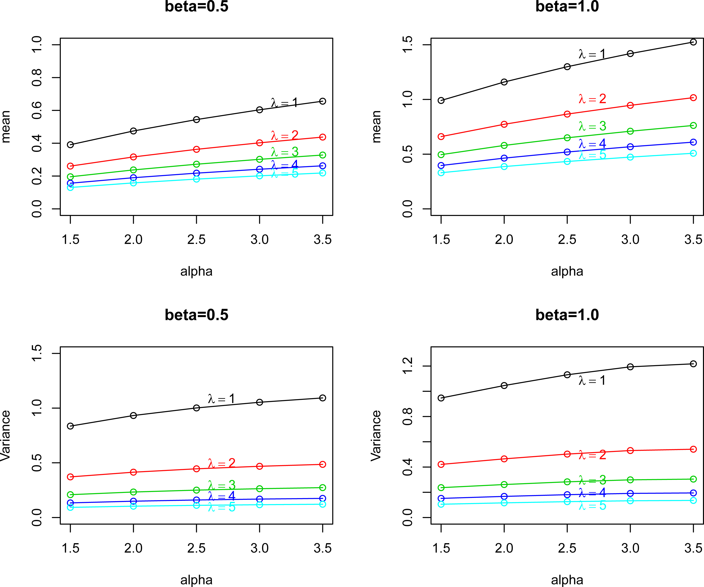
The mean of EP I distribution for $\beta=0.5$ (top left); $\beta=1.0$ (top right) and the variance of EP I distribution for $\beta=0.5$ (bottom left); $\beta=1.0$ (bottom right).

7. Numerical aspects

Here, we investigate how the moments of lower record values from the EP I distribution vary with respect to $\alpha,\beta$ and $\lambda$ . The recurrence relations obtained in the preceding sections allow us to evaluate the means, variances and covariances of all order statistics for all sample sizes in a simple recursive manner and can be used for various inferential purposes; for example, they are useful in determining BLUEs of location/scale parameters and best linear unbiased predictors (BLUPs) of censored failure times. More details on BLUEs and BLUPs based on order statistics can be seen in (Balakrishnan & Cohen, 1991; Arnold et al., 1992).

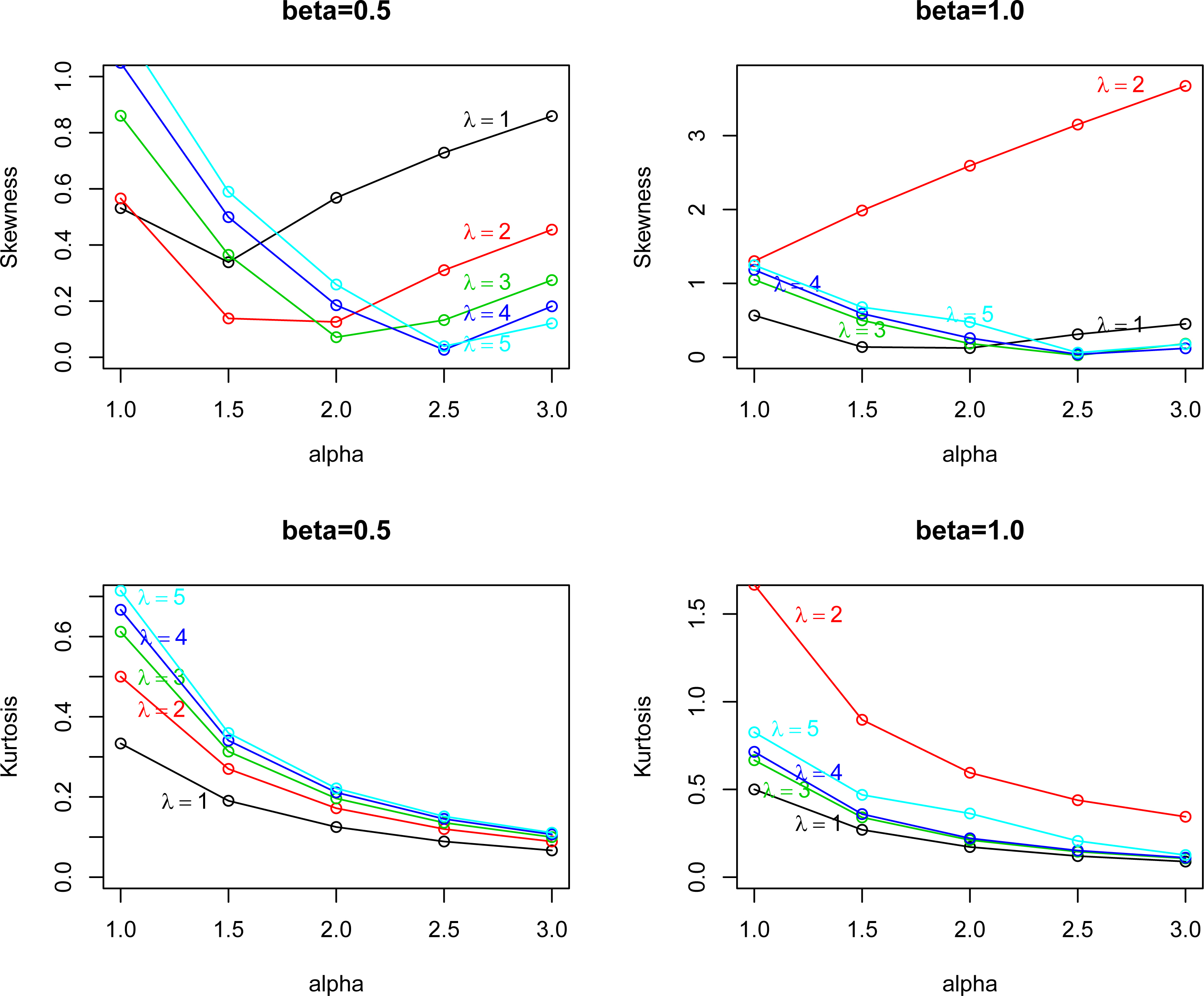
In this section, we plot the mean and variance versus $\alpha$ for selected values of $\beta$ and $\lambda$ . Figure 1 shows the mean and variance versus $\alpha$ and for $\beta=0.5,1.0$ and $\lambda=1(1)5$ . Figure 2 plots the skewness and kurtosis versus $\alpha$ for selected values of $\beta$ and $\lambda$ . Figure 2 shows the skewness and kurtosis $\alpha$ and for $\beta=0.5,1.0$ and $\lambda=1(1)5$ . We see from Fig. 1 that mean and variance of EP I distribution is increasing function of $\alpha$ for selected values of $\beta$ and $\lambda$ . Also we see from Fig. 2 that skewness and kurtosis of EP I distribution is decreasing function of $\alpha$ for selected values of $\beta$ and $\lambda$ .

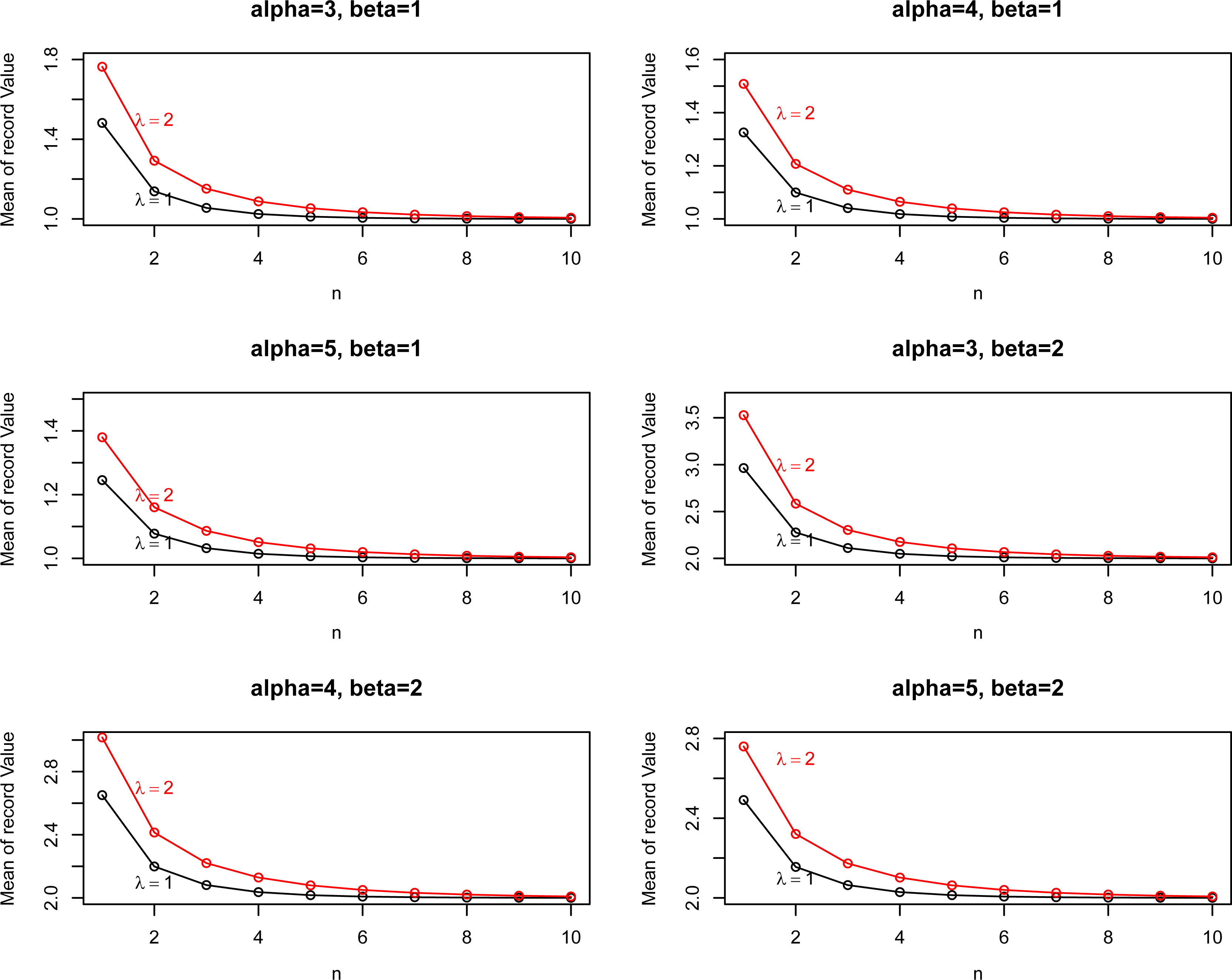
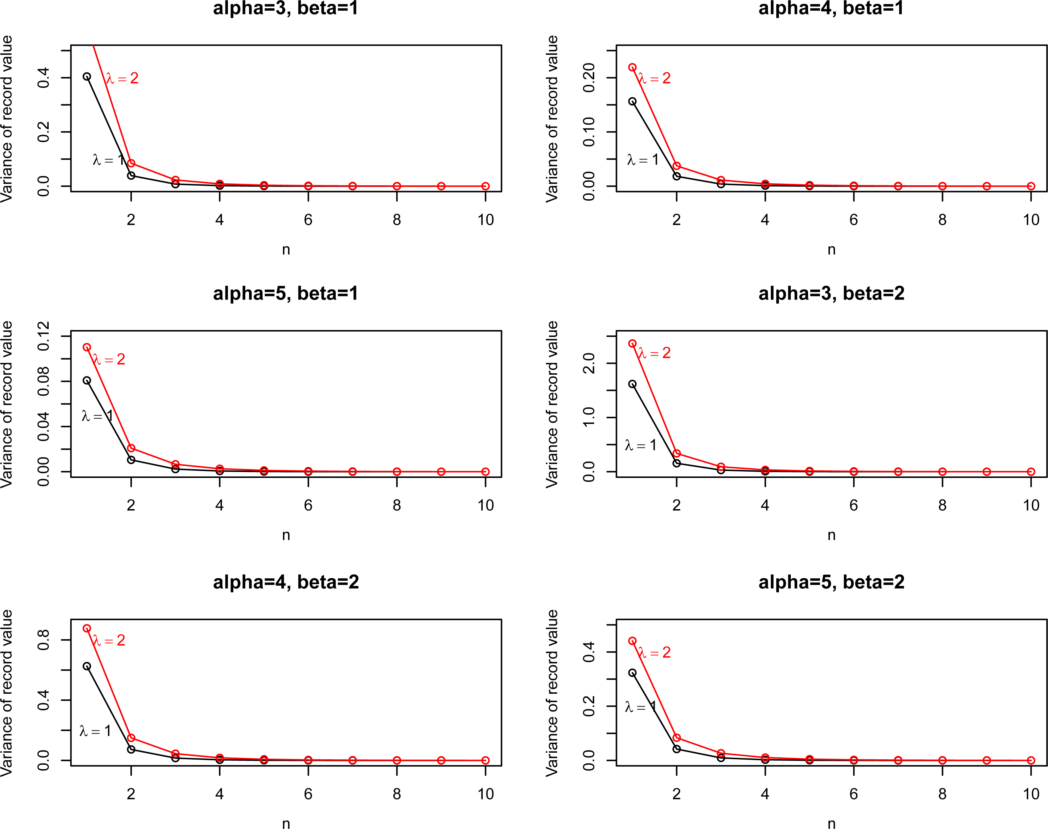
In the rest of the section, we plot the mean, and variance based on record values. From Fig. 3, one can see that the moments are decreasing function with $n$ . Figure 4 shows that the variance are decreasing with respect to $n$ and $\alpha$ but increasing function with $\beta$ and $\lambda$ .

Figures for the skewness, kurtosis, product moments and covariances of record values are not presented here but are available from the authors on request. All computations here were performed using R-Software. R-Software like other algebraic manipulation packages allows for arbitrary precision, so the accuracy of the given values is not an issue.

Figure 2.

The skewness of EP I distribution for $\beta=0.5$ (top left); $\beta=1.0$ (top right) and the kurtosis of EP I distribution for $\beta=0.5$ (bottom left); $\beta=1.0$ (bottom right).

8. EP I model fitting to real data sets

In this section,we use two real data sets to illustrate the estimation and prediction procedures proposed in this work. For computation, we have used R package coda.

We compare the EP I distribution with exponentiated exponential Possion (EEP) distribution (Pogány, 2015), Weibull-Poisson (WP) distribution (Lu & Shi, 2012), complementry exponential geometrc (CEG) distribution (Louzada et al., 2011),

Table 1
Descriptive statistics for data I

	Mean	Median	Mode	SD	Skewness	Kurtosis	Min.	Max.
Data I	14.24	11.2	0	8.39	1.08	3.82	4.10	39.20

Table 2

Prediction of 4-th lower record for data I

Estimation method	$\hat{\alpha}$	$\hat{\beta}$	$\lambda$	$y(.)$
PMLE (data I)	12.6038	38.2501	402.04	417.03
95% predictive interval	(2.085, 21.432)	(11.270, 64.593)	(301.78, 415.03)	(55.021, 458.23)

Table 3

List the MLEs of the models parameters and the approximate confidence intervals of the parameters of the EP I distribution for data I

Model	MLE			CIs
	$\hat{\alpha}$	$\hat{\beta}$	$\hat{\lambda}$	$\alpha$	$\beta$	$\lambda$
Data I	5.1437	1.6024	375.00	(0.6908, 10.9782)	(0.6224, 2.5824)	(374.02, 375.98)

Figure 3.

Mean of EP I distribution based on record values for different values of parameters.

Lindley (LN) distribution (Lindley, 1958). Their density functions (for $x>0$ ) are given by

$\displaystyle\text{EEP}:f(x;\alpha,\beta,\lambda)=\frac{\alpha\beta\lambda}{1-% e^{-\lambda}}e^{-\beta x}\left(1-e^{-\beta x}\right)^{\alpha-1}e^{-\lambda% \left(1-e^{-\beta x}\right)^{\alpha}},∼{}∼{}\alpha,\beta,\lambda>0,$ $\displaystyle\text{WP}:f(x;\alpha,\beta,\lambda)=\frac{\alpha\beta\lambda x^{% \alpha-1}}{1-e^{-\lambda}}e^{-\lambda-\beta x^{\alpha}+\lambda exp(-\beta x^{% \alpha})},∼{}∼{}\alpha,\beta,\lambda>0$ $\displaystyle\text{CEG}:f(x;\lambda,\theta)=\frac{\lambda\theta e^{-\lambda x}% }{[\theta+(1-\theta)e^{-\lambda x}]^{2}},∼{}∼{}\lambda,\theta>0,$ $\displaystyle\text{LN}:f(x;\theta)=\frac{\theta^{2}}{(1+\theta)}(1+x)e^{-% \theta x},∼{}∼{}\theta>0.$

Table 4

List the MLEs of the models parameters and the corresponding standard errors (in parentheses) and the approximate confidence intervals of the parameters of all the models for data I

Model	MLE			CIs
	$\hat{\alpha}$	$\hat{\beta}$	$\hat{\lambda}$	$\alpha$	$\beta$	$\lambda$
EP I	2.0858	0.5528	375.00	(1.6550, 2.5167)	(0.1330, 1.2388)	(374.02, 375.98)
EEP	2.0758	0.1111	0.0272	(0.0988, 4.0525)	(0.0001, 0.2431)	(0.0001, 7.0390)
WP	2.2757	0.0010	3.1550	(2.1719, 2.3796)	(0.0000, 0.9807)	(0.8495, 5.4605)
CEG	0.1952	0.0889		(0.1345, 0.2559)	(0.0039, 0.1724)

Table 5

Goodness-of fit statistics for data I

Model	$-2L$	AIC	BIC	K-S	P-value
EP I	168.9992	343.9983	349.7938	0.06188	0.9880
EEP	174.5937	355.1874	360.9829	0.1450	0.5616
WP	170.9905	347.9810	353.7764	0.0988	0.8768
CEG	174.7967	353.5935	357.4571	0.1007	0.8858

Figure 4.

Variance of EP I distribution based on record values for different values of parameters.

Table 6

Descriptive statistics for data II

	Mean	Median	Mode	SD	Skewness	Kurtosis	Min.	Max.
Data II	121.3	57.0	0	154.27	1.25	4.57	12.0	502

Table 7

Prediction of 6-th lower record for data II

Estimation method	$\hat{\alpha}$	$\hat{\beta}$	$\lambda$	$y(.)$
PMLE (data II)	1.5259	2.6201	398.52	420.12
95% predictive interval	(0.6701, 2.5807)	(0.8807, 4.3709)	(293.78, 408.13)	(67.052, 458.62)

Table 8

List the MLEs of the models parameters and the approximate confidence intervals of the parameters of the EP I distribution for data II

Model	MLE			CIs
	$\hat{\alpha}$	$\hat{\beta}$	$\hat{\lambda}$	$\alpha$	$\beta$	$\lambda$
Data II	0.8823	0.0892	374.99	(0.1066, 1.6579)	(0.0001, 1.6920)	(374.01, 375.97)

Table 9

List the MLEs of the models parameters and the corresponding standard errors (in parentheses) and the approximate confidence intervals of the parameters of all the models for data II

Model	MLE			CIs
	$\hat{\alpha}$	$\hat{\beta}$	$\hat{\lambda}$	$\alpha$	$\beta$	$\lambda$
EP I	1.1440	0.2616	299.99	(0.6807, 1.6072)	(0.0010, 0.9476)	(298.62, 301.36)
EEP	1.1905	0.0056	2.3448	(0.4917, 1.8892)	(0.0015, 0.0128)	(0.0021, 6.2172)
LN	0.0163			(0.0104, 0.0222)

Table 10

Goodness-of fit statistics for data II

Model	$-2L$	AIC	BIC	K-S	P-value
EP I	84.0750	174.1501	176.2742	0.1476	0.9251
EEP	86.0423	178.0846	180.2088	0.2033	0.6604
CEG	86.1541	176.3082	177.7243	0.1909	0.9551
LN	90.6706	183.3412	184.0493	0.3863	0.1813

Figure 5.

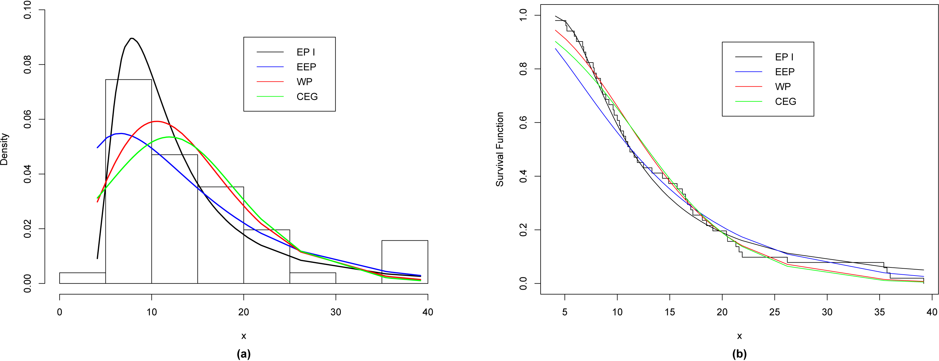
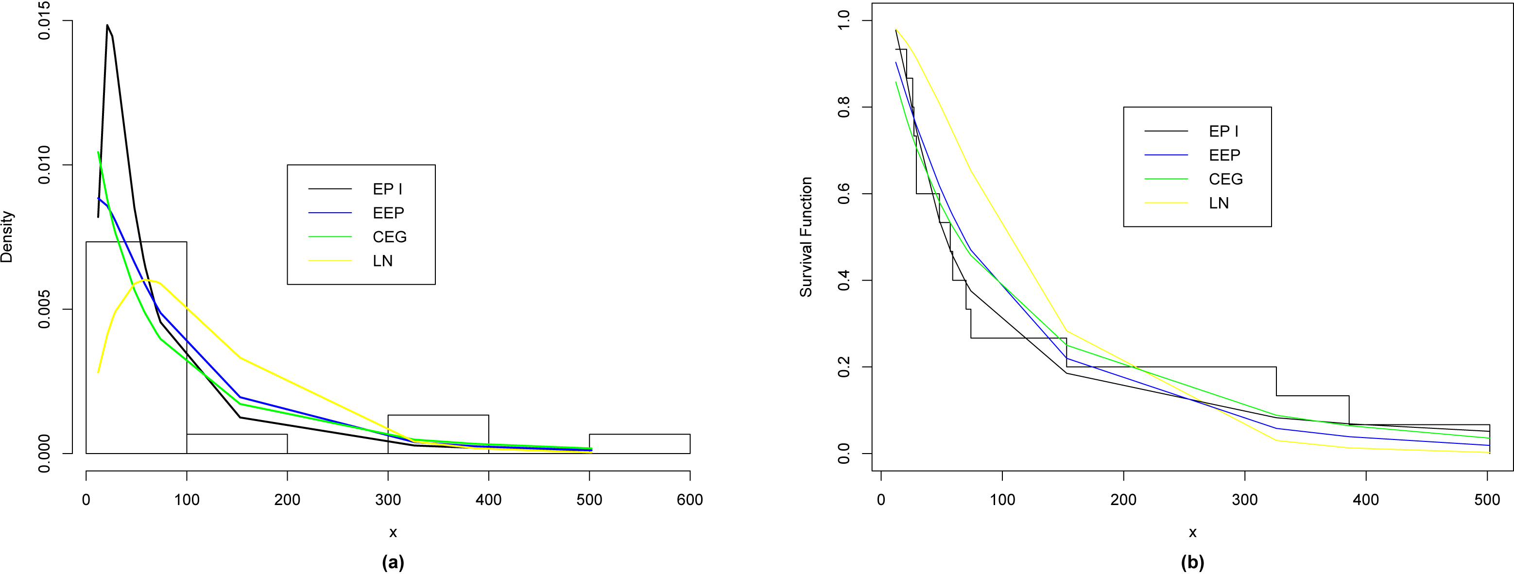
(a) The relative histogram with the fitted distributions for data I, (b) The empirical and fitted survival functions for various distributions for data I.

In order to compare the proposed distribution with the competitive distributions, we use the maximum likelihood method to obtain the values of the goodness of fit statistics $-2L$ where ( $L$ denotes the log-likelihood function evaluated at the maximum likelihood estimates), Kolmogorov-Smirnov (K-S) statistic and the corresponding p-value, Akaike Information Criterion (AIC) and Bayesian Information Criterion (BIC) for data I and data II, respectively.

Figure 6.

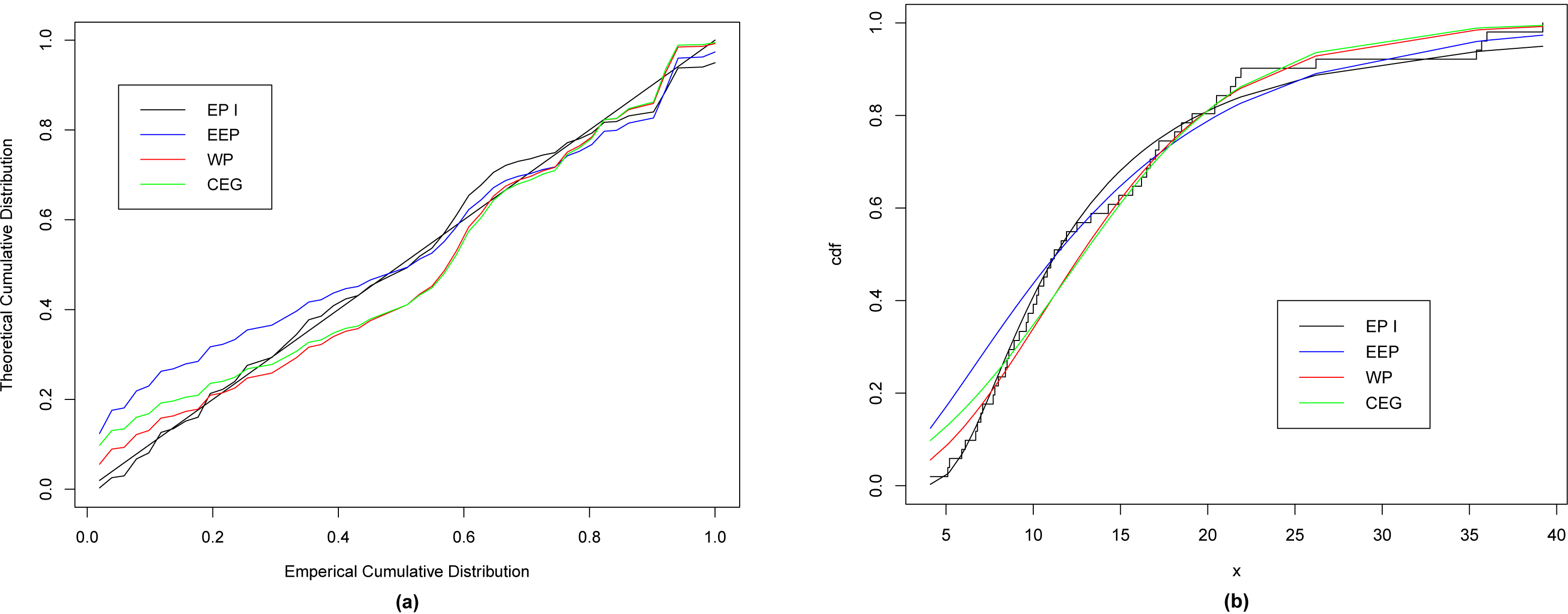
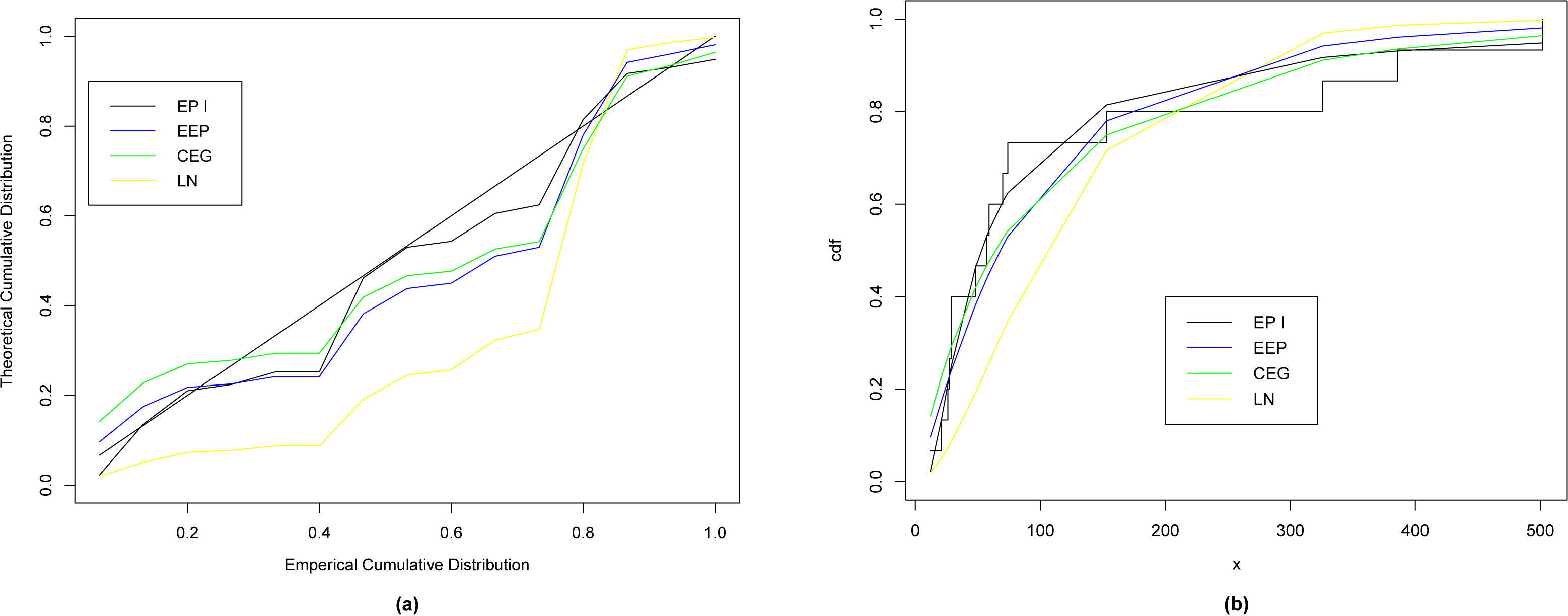
(a) The theoretical and emperical cumulative distribution with the various fitted distributions, (b) The fitted CDF for various distributions.

Figure 7.

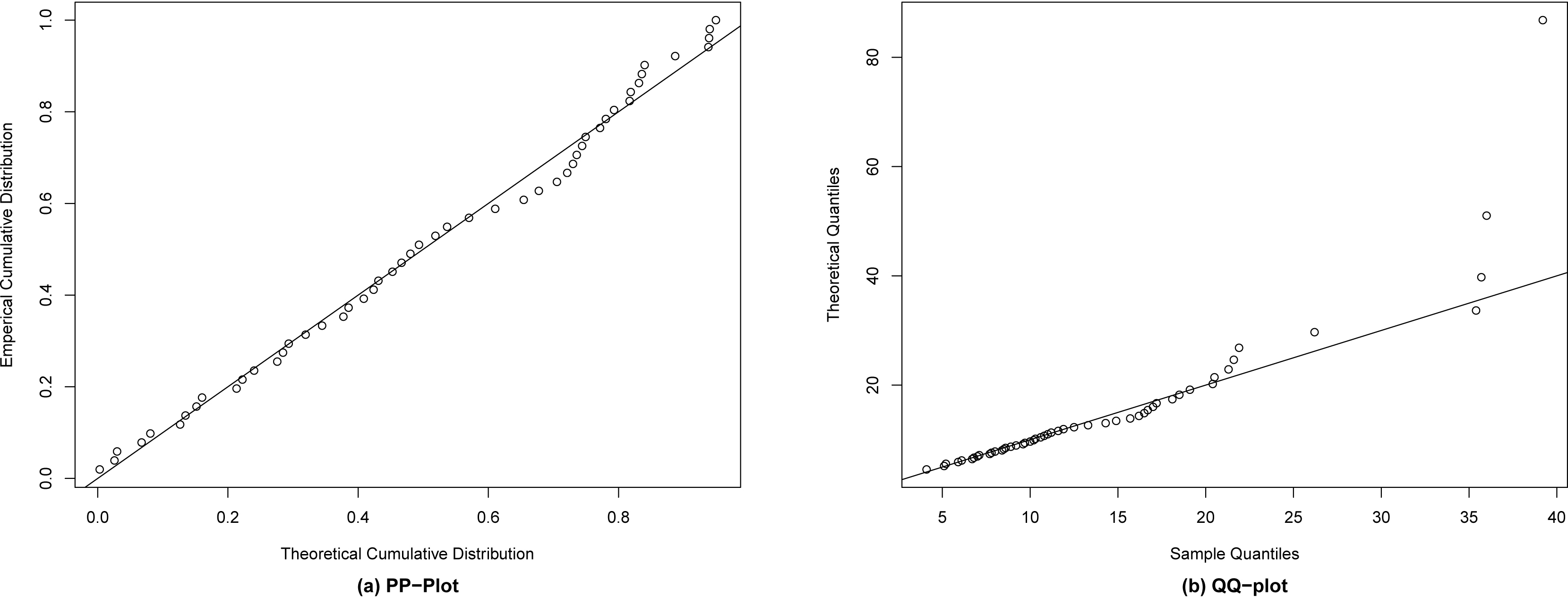
(a) P-P plot for the EP I distribution for data I. (b) Q-Q plot for the EP I distribution for data I.

Figure 8.

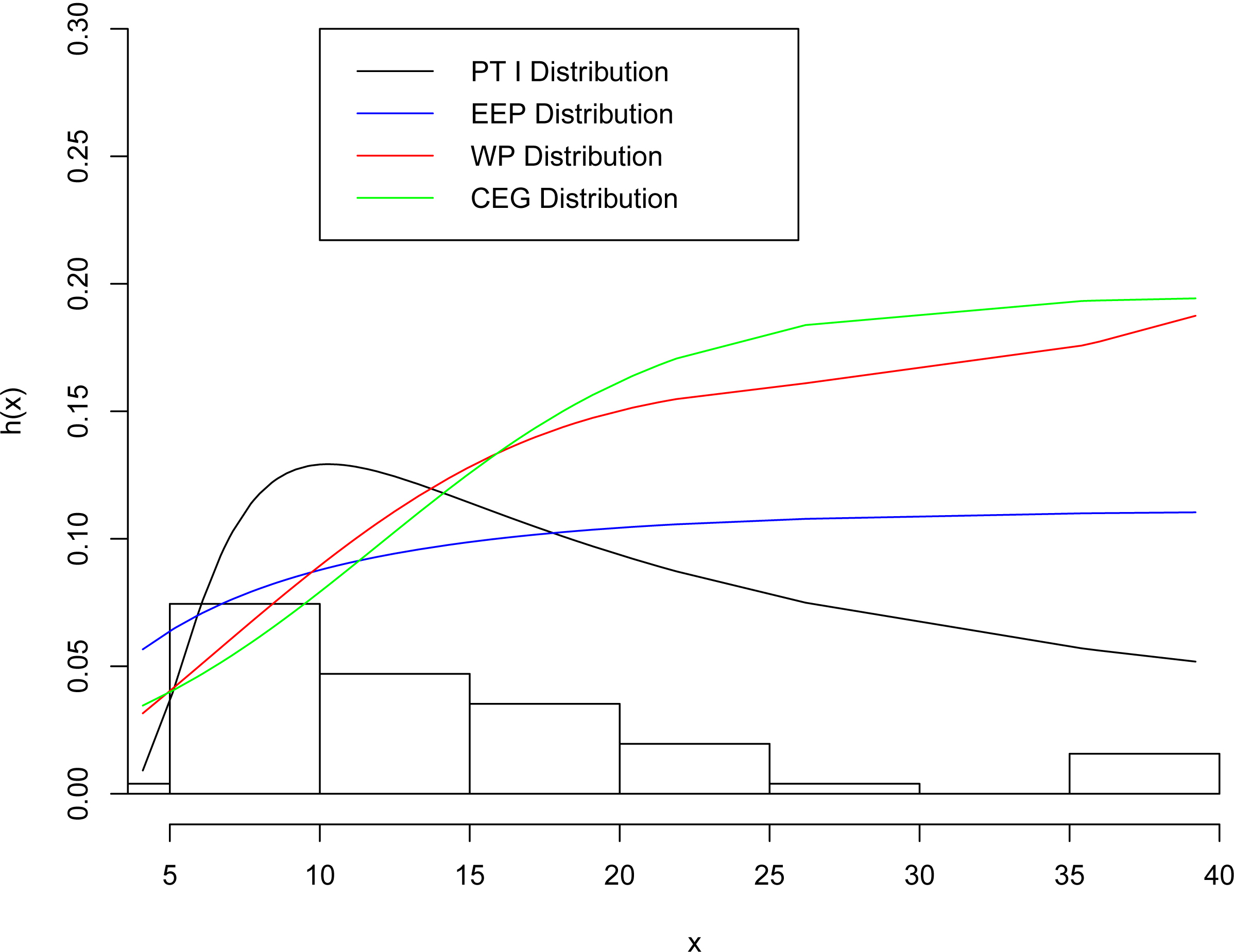
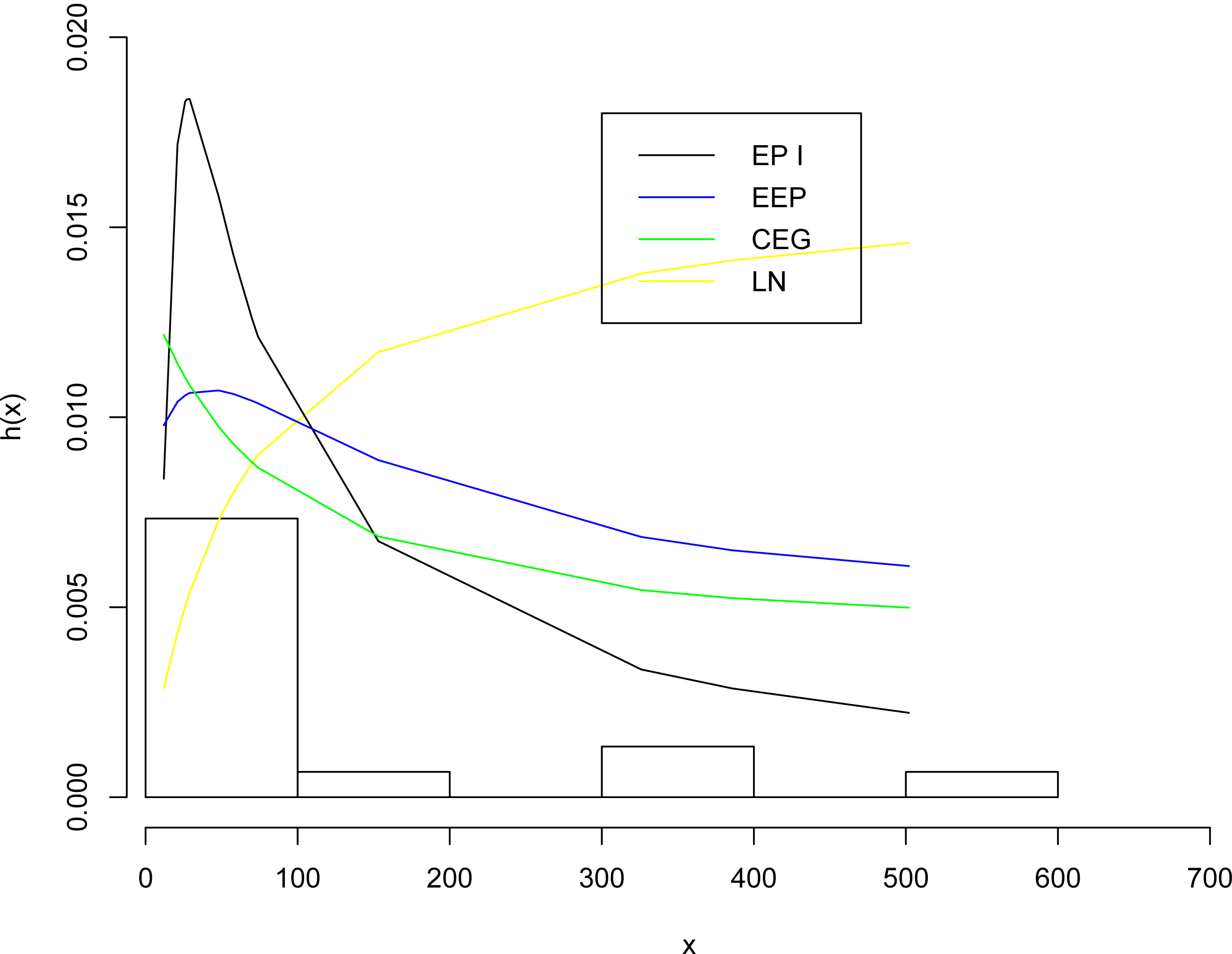
The fitted hazard function for various distributions for data I.

Example 1. The first data set (data I) represents the actual taxes data set. The revenue in Egypt is divided onto 5 chapters and although the taxes is only one chapter from these 5 chapters, but it records the majority of the income. The data consists of the monthly actual taxes revenue in Egypt from January 2006 to November 2010. The distribution is highly skewed to the right. The data (in 1000 million Egyptian pounds) are:

Figure 9.

(a) The relative histogram with the fitted distributions for data II, (b) The empirical and fitted survival functions for various distributions for data II.

5.9, 20.4, 14.9, 16.2, 17.2, 7.8, 6.1, 9.2, 10.2, 9.6, 13.3, 8.5, 21.6, 18.5, 5.1,6.7, 17, 8.6, 9.7, 39.2, 35.7, 15.7, 9.7, 10, 4.1, 36, 8.5, 8, 9.2, 26.2, 21.9,16.7, 21.3, 35.4, 14.3, 8.5, 10.6, 19.1, 20.5, 7.1, 7.7, 18.1, 16.5, 11.9, 7, 8.6,12.5, 10.3, 11.2, 6.1, 8.4, 11, 11.6, 11.9, 5.2, 6.8, 8.9, 7.1, 10.8.

Table 1 gives a descriptive summary of the actual taxes in Egypt from January 2006 to November 2010.

These data were studied by Nassar and Nada (2011) using beta generalized Pareto distribution. But no one has discussed these data set in considered model under lower record values. From this data set we have extracted three lower records 5.9, 5.1, 4.1 for our data analysis. The parameter estimation results are summarized in Table 5. Besides parameter estimation, we have also implemented prediction procedures as mentioned the earlier section of the paper. Here our goal is to predict 4-th lower record value based on the three records considered in the parameter estimation. Table 2 represents our finding from the data analysis.

Figure 10.

(a) The theoretical and emperical cumulative distribution with the various fitted distributions for data II, (b) The fitted CDF for various distributions for data II.

Figure 11.

(a) P-P plot for the EP I distribution for data II, (b) Q-Q plot for the EP I distribution for data II.

Figure 12.

The fitted hazard function for various distributions for data II.

Table 5 lists the values of $-2L$ , AIC, BIC, K-S and p-value, respectively. From Table 5, we observe that the EP I distribution gives the lowest values of $-2L$ , K-S (with largest p-value), AIC and BIC among all fitted models, so it could be chosen as the best model to fit the given data set.

Example 2. The second data set (data II) consist of the times between successive failures of air conditioning equipment in a Boeing 720 airplane. These data were analyzed by Proschan (2000), the data are:

74, 57, 48, 29, 502, 12, 70, 21, 29, 386, 59, 27, 153, 26, 326.

Table 6 gives a descriptive summary of the times between successive failures of air conditioning equipment in a Boeing 720 airplane.

From this original data set we have extracted five lower records 74, 57, 48, 29, 12 for our data analysis. The parameter estimation results are summarized in Table 5. Besides parameter estimation, we have also implemented prediction procedures as mentioned the earlier section of the paper. Here our goal is to predict 6-th lower record value based on the three records considered in the parameter estimation. Table 7 represents our finding from the data analysis.

Table 10 lists the values of $-2L$ , AIC, BIC, K-S and p-value, respectively. From Table 5, we observe that the EP I distribution gives the lowest values of $-2L$ , K-S (with largest p-value), AIC and BIC among all fitted models, so it could be chosen as the best model to fit the given data set.

9. Conclusions

The exponentiated Pareto type I distribution provided excellent model for life time data for a variety of situations. Thus, it is important for the analyst to have reliable statistical methods to use for this distribution. We have provided in this study, a new explicit expressions and recurrence relations for single and product moments of lower record values from the EP I distribition. Further, we have provided frequentist methods of estimating the parameters based on samples of lower record values and methods of predicting future record values.

A future work may be to derive estimation procedures for the EP I distribution based on order statistics, generalized order statistics and dual generalized order statistics. Another future work may be to characterize the EP I distribution based on order statistics, generalized order statistics and dual generalized order statistics.

Footnotes

Acknowledgments

The authors are grateful for the comments and suggestions by the referees and the Co-Editor-in-Chief. Their comments and suggestions have greatly improved the paper.

References

Ahsanullah

(1995). Record Statistics. Nova Science Publishers, New York.

Akinsete

Famoye

, & Lee

(2008). The beta-Pareto distribution. Statistics, 42, 547-563.

Arnold

B. C.

Balakrishnan

, & Nagaraja

H. N.

(1992). A First course in order. John Wiley and Sons, New York.

Mead

M. E.

(2014). An extended Pareto distribution. Pakistan Journal of Statistics and Operation Research, 10, 313-329.

Arnold

B. C.

Balakrishnan

, & Nagaraja

H. N.

(1998). Record. John Wiley and Sons, New York.

Balakrishnan

, & Ahsanullah

(1993). Relations for single and product moments of record values from exponential distribution. J Appl Statist Sci, 2, 73-87.

Balakrishnan

, & Ahsanullah

(1994). Recurrence relations for single and product moments of record values from generalized Pareto distribution. Comm Statist Theory Methods, 23, 2841-2852.

Balakrishnan

, & Cohen

A. C.

(1991). Order statistics and inference: Estimation methods. Boston, MA:Academic Press.

Basak

, & Balakrishnan

(2003). Maximum likelihood prediction of future record statistic, in: Lindquist

B. H.

, & Doksum

K. A.

(eds), Mathematical and Statistical Methods in Reliability, in: Series on Quality, Reliability and Engineering Statistics, Vol. 7, World Scientific Publishing, Singapore, pp. 159-175.

10.

Bonferroni

C. E.

(1930). Elmenti di statistica generale. Libreria Seber, Firenze.

11.

Burroughs

S. M.

, & Tebbens

S. F.

(2001). Upper-truncated power law distributions. Fractals, 9, 209-222.

12.

Chandler

K. N.

(1952). The distribution and frequency of record values. J Roy Statist Soc, Ser B, 14, 220-228.

13.

Grunzien

, & Szynal

(1997). Characterization of uniform and exponential distributions via moments of the k-th record values with random indices. Appl Statist Sci, 5, 259-266.

14.

Glick

(1978). Breaking records and breaking boards. Arner Math Monthly, 85, 2-26.

15.

Gradshteyn

I. S.

, & Ryzhik

I. M.

(2014). Tables of Integrals, Series of Products. Academic Press, New York.

16.

Gupta

R. C.

Gupta

R. D.

, & Gupta

P. L.

(1998). Modeling failure time data by Lehman alternatives. Comm Statist Theory Methods, 27, 887-904.

17.

Kenney

J. F.

, & Keeping

(1962). Mathematics of Statistics. D Van Nostrand Company.

18.

Khan

R. U.

, & Kumar

(2010). On moments of lower generalized order statistics from exponentiated Pareto distribution and its characterization. Applied Mathematical Sciences, 4, 2711-2722.

19.

Kumar

(2015). Explicit expressions and statistical inference of generalized rayleigh distribution based on lower record values. Mathematical Methods of Statistics, 24, 225-241.

20.

Kumar

Jain

, & Gupta

(2015). The type I generalized half logistic distribution based on upper record values. Journal of Probability and Statistics, 2015, 1-11.

21.

Kumar

(2016). kth lower record values from of Dagum distribution. Discussiones Mathematicae Probability and Statistics, 36, 25-41.

22.

Kumar

(2017). The Singh-Maddala distribution: Properties and estimation. Int J Syst Assur Eng Manag, 8, 1297-1311.

23.

Kumar

Saran

, & Jain

(2017). The Kumaraswamy-Burr III distribution based on upper record values. American Journal of Mathematical and Management Sciences, 36, 205-228.

24.

Lindley

D. V.

(1958). Fiducial distributions and Bayes’s theorem. Journal of the Royal Society, Series B, 20, 102-107.

25.

Louzadaa

Romana

, & Canchob

V. G.

(2011). The complementary exponential geometric distribution: Model, properties, and a comparison with its counterpart. Computational Statistics and Data Analysis, 55, 2516-2524.

26.

, & Shi

(2012). A new compounding life distribution: The Weibull-Poisson distribution. Journal of Applied Statistics, 39, 21-38.

27.

Moors

J. J. A.

(1988). A quantile alternative for kurtosis. Journal of the Royal Statistical Society, Series D (The Statistician), 37, 25-32.

28.

Nassar

M. M.

, & Nada

N. K.

(2011). The beta generalized Pareto distribution. Journal of Statistics: Advances in Theory and Applications, 6, 1-17.

29.

Nevzorov

V. B.

(1987). Records. Theo Prob Appl, 32, 201-228.

30.

Pog

T. K.

(2015). The exponentiated exponential Poisson distribution revisited. Statistics, 49, 918-929.

31.

Proschan

(2000). Theoretical explanation of observed decreasing failure rate. Technometrics, 42, 7-11.

32.

Pickands

(1975). Staistical inference using extreme order statistics. Ann Statist, 3, 119-131.

33.

Resnick

S. I.

(1973). Extreme values, regular variation and point processes. Springer-Verlag, New York.

34.

Schroeder

Damouras

, & Gill

(2010). Understanding latent sector error and how to protect against them. ACM Transactions on Storage (TOS), 6, Article 8.

35.

Shaked

, & Shanthikumar

J. G.

(1994). Stochastic orders and their applications. Boston, MA: Academic Press.

36.

Jain

M. K.

Iyengar

S. R. K.

, & Jain

R. K.

(1984). Numerical Methods for Scientific and Engineering Computation. New Age International Pvt Limited, New Delhi.

37.

Rao

G. S.

(2006). Numerical Analysis. New Age International Pvt Limited, New Delhi.

38.

Shorrock

R. W.

(1973). Record values and inter-record times. J Appl Probab, 10, 543-555.

Record values from exponentiated Pareto type I distribution and associated inference

Abstract

Keywords

1. Introduction

3.1 Quantile function

3.2.1 Ordinary, central and factorial moments

3.4 Conditional moments

3.8 Order statistics

3.9 Joint distribution of the i th and j th order statistics

4.1 Relations for single moments

5.1 Maximum likelihood estimation

6. Prediction of future record values

Table 1 Descriptive statistics for data I

Footnotes

Acknowledgments

References

3.9 Joint distribution of the $i$ th and $j$ th order statistics

Table 1
Descriptive statistics for data I