Applications of Box-Jenkins (Seasonal ARIMA) and GARCH models to dengue incidence in Thailand

Abstract

In this paper, we focus on monthly number of dengue cases in Thailand using the univariate Box-Jenkins (seasonal ARIMA) and GARCH models. There are 3 types of dengue i.e. dengue fever (DF), dengue hemorrhagic fever (DHF), and dengue shock syndrome (DSS). These series are fitted with adjustment by population size and seasonal index. For each type, the best model is choosen by Akaike’s Information Criteria (AIC) and Schwartz’s Bayesian Criteria (SBC). A comparison of the fitted Box-Jenkins and GARCH models are presented using root mean square error (RMSE) and mean absolute percentage error (MAPE). The results showed that the best fitted for the univariate Box-Jenkins models of DF, DHF and DSS cases are seasonal ARIMA(0, 1, 1) $\times$ (0, 1, 1) ${}_{12}$ , ARIMA(0, 1, 1) $\times$ (0, 1, 1) ${}_{12}$ and ARIMA(0, 1, 3) $\times$ (0, 1, 1) ${}_{12}$ , respectively, while the best fitted GARCH models of DF, DHF and DSS cases are AR(1)-GARCH(1, 1) adjusted seasonal components, AR(8)-ARCH(1) removed seasonal components and AR(1)-ARCH(1) adjusted seasonal components, consequently. Further, from a comparison the GARCH model outperforms than the univariate Box-Jenkins (seasonal ARIMA) model. Removing seasonal components technique increased efficiency of fitting model in GARCH method while adjustment by population size did not give a significantly difference result to both methods.

Keywords

Dengue fever dengue hemorrhagic fever dengue shock syndrome population size seasonal index

1. Introduction

Dengue fever also known as breakbone fever, is an infectious caused by the dengue virus. The dengue viruses are members of the genus Flavivirus in the family Flaviviridae and are divided into 4 serotypes, i.e. DEN-1, DEN-2, DEN-3 and DEN-4. Dengue symptoms are classified into three groups: dengue fever (DF), dengue hemorrhagic fever (DHF), and dengue shock syndrome (DSS). Dengue infection spreads to people by mosquitoes Aedesaegypti. The symptoms of disease are fever, headache, and muscle and joint pain, which are all very similar to those of fever-causing illness. Recently, dengue has emerged as a substantial global health problem with increased incidences in new countries and tropical areas (Nimmanpipaknit, 1997).

Dengue virus outbreak in Thailand since 1958 (Gubler & Kuno, 1997), then the disease is a major health problem in the country ever since. The outbreak was dengue fever (DF) and dengue hemorrhagic fever (DHF), every 2–3 years until the outbreak of violence in 1987 and 1998 (Punthana, 1999). In 1998, there were about 120,000 cases of dengue with 400 dead cases where DF was 85 percent, DHF was 13 percent and DSS was 1.86 percent (Bureau of the vector-borne diseases, 2014). In 2013, the number of the total cases was 154,444 cases (incidence rate is 241.03 per hundred thousand) and the number of the deaths was 136 cases (fatality rate is 0.09 percent). Then, Ministry of Public Health has taken some turn center emergency responders, Bureau of the vector-borne diseases, 2014.

The Box-Jenkins approach was described by statisticians George Box and Gwilym Jenkins in 1970. The Box-Jenkins approach uses to model autoregressive integrated moving average (ARIMA) process which is a mathematical time series model and used for forecasting the series. Data in time series are frequently collected at weekly or monthly intervals, e.g. notifications of diseases, entries to a hospital, mortality rates etc. often arise in the form of time series (Catalano et al., 1987; Helfenstein, 1991). The ARIMA models have been used successfully in epidemiology to monitor and predict infectious diseases, such as malaria and hepatitis A incidence, influenza and pneumonia deaths, accompany by other infectious diseases incidences, and the use of health facilities, or isolation beds (Earnest et al., 2005). Especially, the ARIMA model are used to forecast the dengue (Promprou et al., 2006; Paula et al., 2008; Siriwan et al., 2008).

Moreover, the seasonal autoregressive integrated moving average (Seasonal ARIMA) model is useful in situations when the time series data exhibit seasonality-periodic fluctuations that recur with about the same intensity each year and have been shown to be more accurate than those obtained by other statistical methods (Martinezl et al., 2011). (See also Choudhury et al., 2008; Silawan et al., 2008; Martinezet et al., 2011; Bhatnagar et al., 2012; Kavinga et al., 2013).

Further, generalized autoregressive conditional heteroskedasticity (GARCH) model, are used to characterize and model observed time series when the variances of data are not constant, depend on time, or be heteroscedasticity (Bollerslev, 1986). Some authors developed this model to the series in many fields which its variances are depending on time such as Reinaldo et al., (2005); Ranjit et al., (2009); Kiatekarunya, (2011); Siti et al., (2011); Pung et al., (2013). In our study, the number of dengue cases has nonconstant variance. Hence, the GARCH procedure could be used to forecast the dengue incidence in Thailand.

Therefore, the aims of this paper are developing the univariate Box-Jenkins and GARCH models to forecast the dengue incidence in Thailand and comparing the results from both GARCH and Box-Jenkins models. The paper is organized as follows. The first section is an introduction. Methodology is presented in Section 2. Results of the Box-Jenkins and GARCH models are shown in Section 3. Comparison of fitted models are presented in Section 4, while forecasting is presented in Section 5. Finally, the Section 6 shows conclusion.

2. Methodology

2.1 Datasets

The monthly number of dengue cases in Thailand was obtained from Department of Disease Control, Ministry of Public Health. The dataset was divided into two parts: the data observed from January 2003 to June 2013 was used to develop the time series model, and the monthly number of dengue cases from July to December 2013 was used to validate the model.

In this study, we consider the monthly number of dengue cases in Thailand adjusted by population size because in real life, the population size in Thailand varies in each month (Bureau of registration administration, 2014). Let $Zp_{t}$ be the series adjusted by population size at time $t$ , $Z_{t}$ be the dengue series at time $t$ , and $p_{t}$ be the population size at time $t$ .

Moreover, we also consider the monthly number of dengue cases in Thailand adjusted by the seasonal components on the GARCH method since the GARCH model does not have a seasonal component but our data have the seasonal effect. The seasonal indexs are computed by the ratio-to-moving-average method. The $Zs_{t}$ is the seasonal adjusted series at time $t$ and $S_{m}$ is the seasonal index at month $m,m=1,2,\ldots,12$ . While $Zps_{t}$ is the series adjusted by both population size and seasonal index at time $t$ .

2.2 Models

2.2.1 Seasonal ARIMA

Let ${Z}^{\prime}=({Z_{1},Z_{2},\ldots,Z_{t}})$ be a time series data. A Seasonal ARIMA model with the subindex $s$ refers to the seasonal period, denoted by ARIMA( $p, d, q$ ) $\times$ ( $P, D, Q$ ) ${}_{s}$ is given by $\Phi_{P}(B^{s})\phi_{p}(B)({1-B})^{d}({1-B^{s}})^{{}^{D}}\dot{{Z}}_{t}=\theta_% {q}(B)\Theta_{Q}(B^{s})a_{t},$ where $B$ is the backward shift operator given by $B^{j}x_{t}=x_{t-j}$ . Further, $\phi_{p}(B)=1-\phi_{1}B^{1}-\phi_{2}B^{2}-\ldots-\phi_{p}B^{p}$ is an autoregressive (AR) polynomial function of order $p$ with vector of coefficients ${\phi}^{\prime}=(\phi_{1},\phi_{2},\ldots,\phi_{p})$ , and $\theta_{q}(B)=1+\theta_{1}B^{1}+\theta_{2}B^{2}+\ldots+\theta_{q}B^{q}$ is a moving average (MA) polynomial of order $q$ with vector of coefficients ${\theta}^{\prime}=(\theta_{1},\theta_{2},\ldots,\theta_{q})$ . $\Phi_{P}({B^{S}})=1-\Phi_{1}B^{S}-\Phi_{2}B^{2S}-\ldots-\Phi_{P}B^{PS}$ , and $\Theta_{Q}({B^{S}})=1-\Theta_{1}B^{S}-\Theta_{2}B^{2S}-\ldots-\Theta_{Q}B^{QS}$ are seasonal polynomial functions of order $P$ and $Q$ , respectively, which satisfy the stationarity and invertibility conditions, $d$ is the number of differencing passes needed to stationarize the series, $D$ is the number of seasonal differences and $a_{t}$ are error terms assumed to be independent identically distributed random variables sampled from a distribution with a zero mean and the variance is $\sigma_{a}^{2}$ . In addition, the adequacy of each model was verified by a sample autocorrelation (ACF) of the standardized residuals and the Ljung-Box test (Wei, 2006).

2.2.2 GARCH model

The GARCH or generalized autoregressive conditional heteroscedastic model is used to fit the series which its variance is not constant or depends on time. This section describes the ARCH model and the traditional GARCH model as the following.

2.2.3 ARCH model

The ARCH( $q$ ) model was proposed by Engle (1982). It addresses the heteroskedasiticity in the data over time and models this explicitly in terms of defining a model for conditional variance. The conditional density function $f({Z_{t}|{Z_{t-1}}})$ represents the prediction of current random variable $Z_{t}$ which is based upon the past information. The conditional variance denoted by $Var({Z_{t}|{Z_{t-1}}})$ depends on the past information and changes within the time. In 1982, Engle presented ARCH model under the assumption of normality with zero mean as:

$Z_{t}=\varepsilon_{t}\sqrt{h_{t}};h_{t}=\omega+\sum\limits_{i=1}^{q}{\alpha_{i% }\varepsilon_{t-i}^{2}},$

where $Z_{t}|{\psi_{t-1}\sim N(0,h_{t})},\psi_{t-1}$ is the information set at time $t-1$ , $q$ is the order of ARCH process, $\omega$ and $\alpha_{i}$ are unknown parameters, $\varepsilon_{t}$ is an error term often assumed to be i.i.d. $N(0,\sigma_{\varepsilon}^{2}),$ and $h_{t}$ is the conditional variance which depends on the past time $t-i$ .

To extend the model, Engle (1982) assumed that the mean of conditional density function of $Z_{t}$ is ${x}^{\prime}_{t}b$ , a linear combination of lagged endogenous and exogenous variables, which included past information set $\psi_{t-1}$ with a vector of unknown parameters $b$ . It can be formally expressed as:

$Z_{t}={x}^{\prime}_{t}b+\varepsilon_{t};\varepsilon_{t}=e_{t}\sqrt{h_{t}};h_{t% }=\omega+\sum\limits_{i=1}^{q}{\alpha_{i}\varepsilon_{t-i}^{2}},$

where $Z_{t}|{\psi_{t-1}\sim N({x}^{\prime}_{t}b,h_{t})},e_{t}\sim N(0,1),x_{t}$ is a vector of explanatory variables, $b$ is a vector of unknown regression parameter, $q$ is the order of ARCH process, $\omega$ and $\alpha_{i}$ are unknown parameters, $\varepsilon_{t}$ is an error term often assumed to be i.i.d. $N(0,\sigma_{\varepsilon}^{2}),$ and $h_{t}$ is the conditional variance which depends on the past time.

To ensure that the conditional error variance, $h_{t},$ is positive, the restrictions that $\omega>0$ and $\alpha_{i}\geqslant 0,i=1,2,\ldots,q,$ are imposed. Engle shows that when $\sum\nolimits_{i=1}^{q}{\alpha_{i}}<1,$ the ARCH( $q$ ) model has positive and finite unconditional variance $\textit{Var}(\varepsilon_{t})=\omega/(1-\sum\nolimits_{i=1}^{q}{\alpha_{i})}.$

2.2.4 Traditional GARCH model

Bollerslev (1986) introduced a new general class of ARCH models, named generalized autoregressive conditional heteroscedastic (GARCH) models, which allows for both a long memory and a more flexible lag structure. ARCH models concern with the conditional variance which is linearly associated with the past variances only. The GARCH models added the previous conditional variances into the formulation as well. The GARCH model with the assumption of normality can be expressed as

$Z_{t}={x}^{\prime}_{t}b+\varepsilon_{t};h_{t}=\omega+\sum\nolimits_{i=1}^{q}{% \alpha_{i}}\varepsilon_{t-i}^{2}+\sum\nolimits_{j=1}^{p}{\beta_{j}h_{t-1}}$

where $p\geqslant 0;q>0;\omega>0;\alpha_{i}\geqslant 0,i=1,2,3,\ldots,q;\beta_{j}% \geqslant 0,j=1,2,3,\ldots,p;q$ is the order of moving average ARCH terms, $p$ is the order of autoregressive GARCH terms, $\alpha$ and $\beta$ are the vectors of unknown parameters, and $\varepsilon_{t}$ is an error term often assumed to be i.i.d. $N(0,\sigma_{\varepsilon}^{2}).$ Notice that, when $p=$ 0, the GARCH( $p, q$ ) model will be reduced to the ARCH $(q)$ model.

Figure 1.

The sample ACF and PACF for the square root transformed monthly number of DF cases.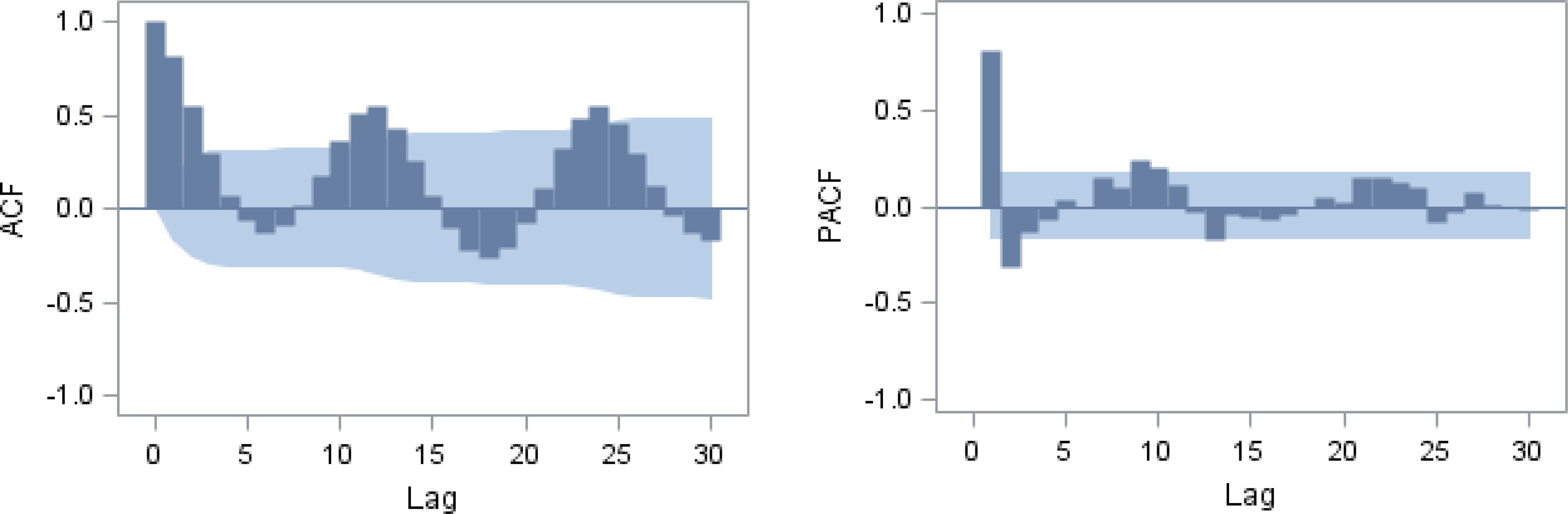

Figure 2.

The sample ACF and PACF for the first differencing of the square root transformed monthly number of DF cases.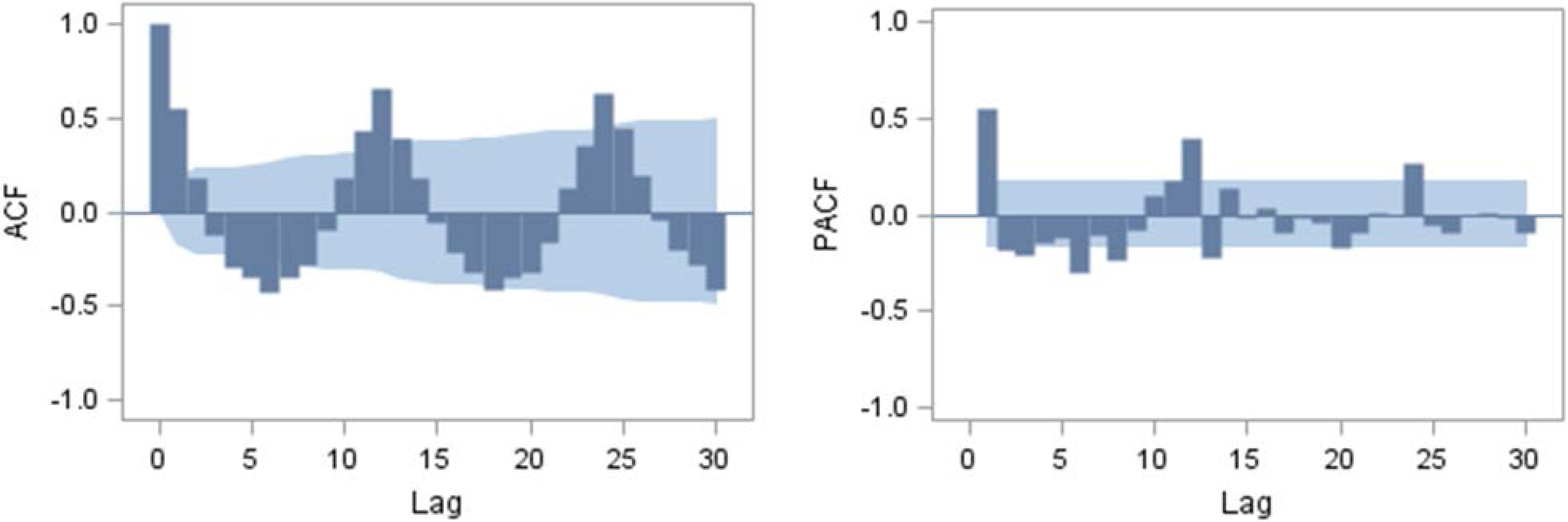

Figure 3.

The sample ACF and PACF for the differencing at period 12 months of the square root transformed monthly number of DF cases.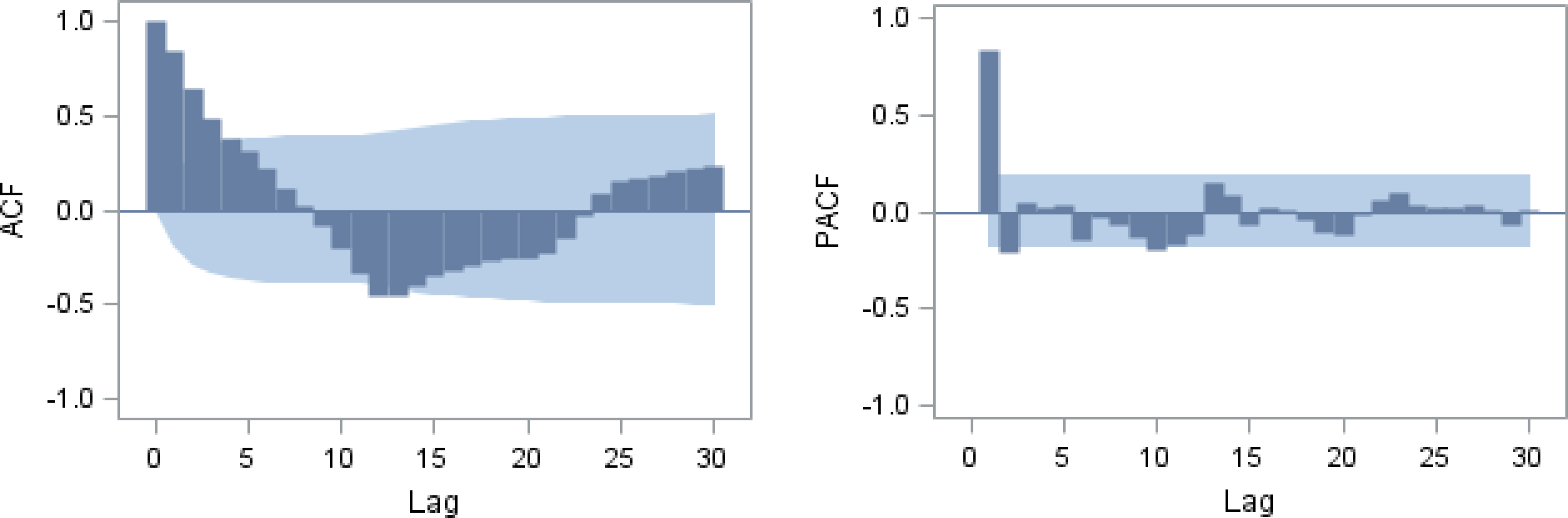

Figure 4.

The sample ACF and PACF for the differencing at periods 1 and 12 months of the square root transformed monthly number of DF cases.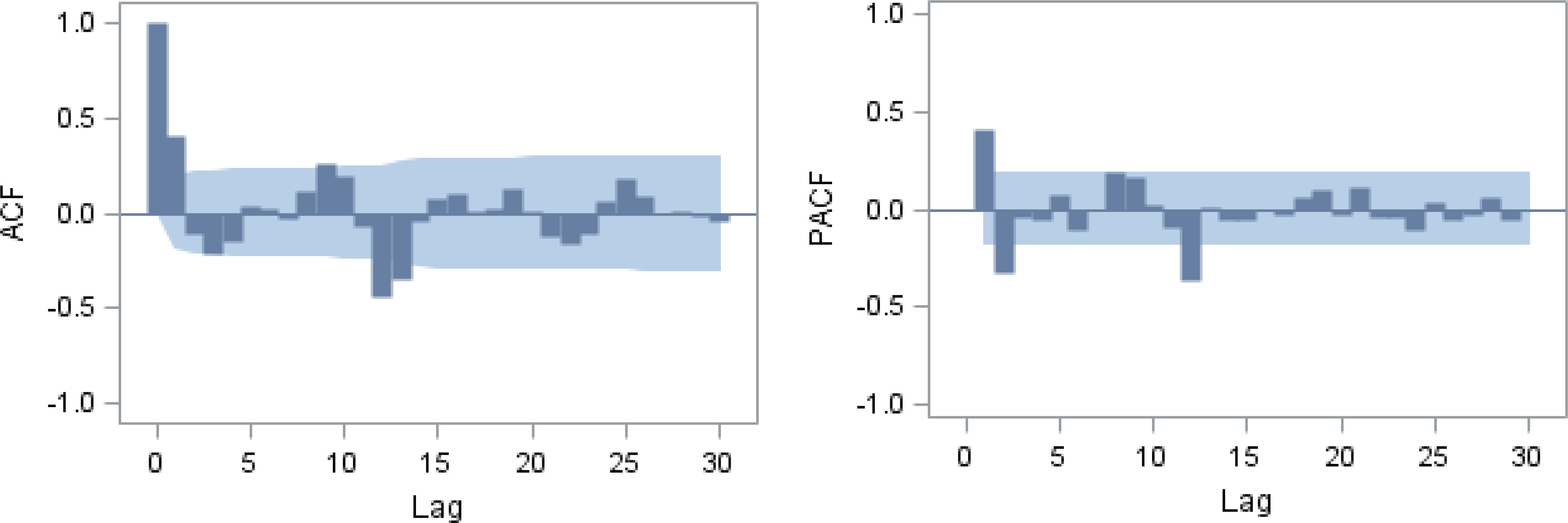

Figure 5.

The residual ACF and PACF for the ARIMA(0, 1, 0) 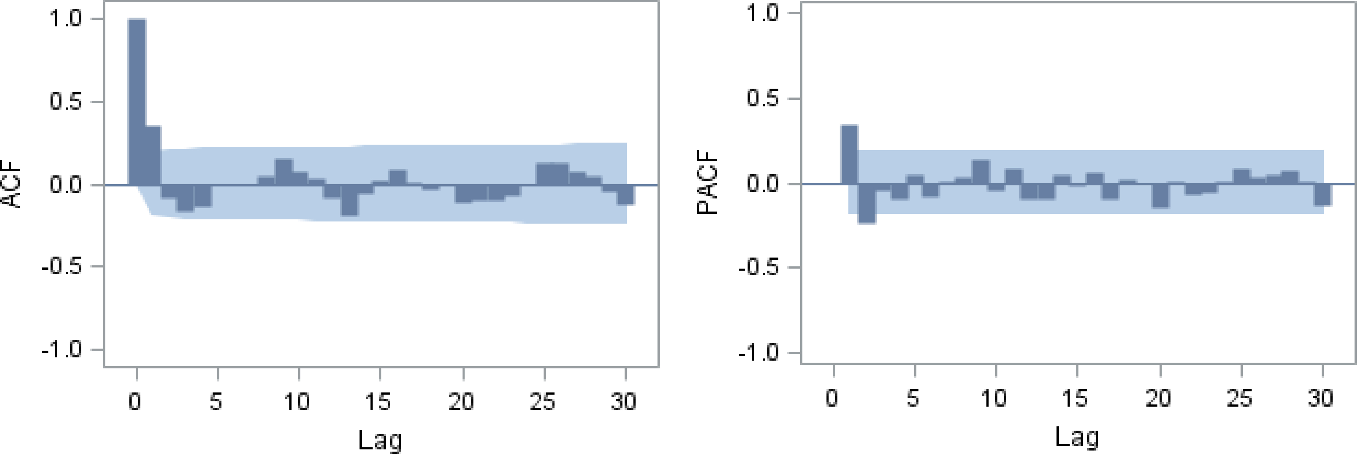$\times$ (0, 1, 1) ${}_{12}$ of the square root transformed monthly number of DF cases.

3. Results

The analysis of three-time series datasets, the monthly number of DF, DHF, and DSS cases by the univariate Box-Jenkins and GARCH models with the techniques of adjustment by population sizes and removing seasonal components are shown in this section. We used SAS ${}^{\@setsize{\scriptsize}{8pt}{\viipt}{\@viipt}\textregistered}$ software version 9.3 to process the Autoregressive Integrated Moving Average (ARIMA) and GARCH models for fitting and forecast these series. To choose the best model for each technique, we used the model selection criteria, i.e. an Akaike’s Information Criteria (AIC) and Schwartz’s Bayesian Criteria (SBC).

3.1 The univariate Box-Jenkins model for DF, DHF, and DSS cases

We investigate whether the series is stationary in the variance by the Box-Cox power transformation. The results showed that series of the monthly number of DF, DHF, and DSS cases need squared root transformation since $\lambda=$ 0.5 gave minimum RMSE for all three series.

The sample ACF and sample PACF for the square root transformed monthly numbers of DF cases are shown in Fig. 1. The sample ACF shows a damped sine-cosine wave and the sample PACF has large spikes at lags 1, 2 and 13. The sample ACF and sample PACF for the first differencing of the square root transformed monthly number of DF cases are shown in Fig. 2. The samples ACF shows a damped sine-cosine wave with large spikes at 12 and 24. Then we consider the differencing at a period 12 months. The sample PACF has large spikes at lags 1, 12 and 13.

The sample ACF and sample PACF for the differencing at period 12 months of the square root transformed monthly number of DF cases are shown in Fig. 3. The sample ACF tends to decrease slowly implies that it needs the first differencing and the sample PACF has large spikes at lags 1 and 2.

To ensure that the first and the twelfth differencing are needed, we consider the sample ACF and PACF for the differencing at period 1 and 12 months of the square root transformed monthly number of DF cases which are shown in Fig. 4. The sample ACF has significant spikes at lags 1 and 12. Hence we identify the following ARIMA(0, 1, 0) $\times$ (0, 1, 1) ${}_{12}$ process as a tentative model for the series.

To identify the nonseasonal components of the ARIMA model the residual ACF and PACF of the ARIMA(0, 1, 0) $\times$ (0, 1, 1) ${}_{12}$ are considered and shown in Fig. 5. The residual ACF has a significant spike at lag 1. The residual PACF has significant spikes at lags 1 and 2. Hence all the tentative models are ARIMA(1, 1, 0) $\times$ (0, 1, 1) ${}_{12}$ , ARIMA(0, 1, 1) $\times$ (0, 1, 1) ${}_{12}$ , ARIMA(1, 1, 1) $\times$ (0, 1, 1) ${}_{12}$ , ARIMA(2, 1, 0) $\times$ (0, 1, 1) ${}_{12}$ , and ARIMA(2, 1, 1) $\times$ (0, 1, 1) ${}_{12}$ .

Parameters of the tentative models are estimated at $p$ -value $<$ 0.05. The values in the parentheses under each estimate refer to the standard errors of these estimators. To check model adequacy, we consider whether the residuals of the tentative models are white noise by using a chi-square statistic with K $=$ 24. We process in the same manner for the monthly number of DHF and DSS cases to obtain the best model. According to the minimum AIC and SBC the best model for the monthly number of DF, DHF, DSS cases are shown in Table 1.

Table 1
The best models for monthly DF, DHF and DSS cases

Model	Estimated parameters	$\hat{{\sigma}}_{a}^{2}$
DF:	ARIMA(0, 1, 1) $\times$ (0, 1, 1) ${}_{12}$
	$(1-B)(1-B^{12})\sqrt{Z_{t}}=(1+0.51163B)(1-0.73486B^{12})a_{t}$	24.45198
	$(0.08339)$ $(0.07659)$
DHF:	ARIMA(0, 1, 1) $\times$ (0, 1, 1) ${}_{12}$
	$(1-B)\sqrt{Z_{t}}=(1+0.29682B)(1-0.8386B^{12})a_{t}$	29.11547
	$(0.09182)$ $(0.05981)$
DSS:	ARIMA(0, 1, 3) $\times$ (0, 1, 1) ${}_{12}$
	$(1-B)(1-B^{12})\sqrt{Z_{t}}=(1+0.21128B-0.3255B^{3})(1-0.69919B^{12})a_{t}$	2.178166
	$(0.08882)$ $(0.08854)$ $(0.07169)$

3.2 The univariate Box-Jenkins model adjusted by population size

In the same manner using the ARIMA model but the data sets in this section were adjusted by population size ( $Zp_{t}$ ). The best monthly number of DF, DHF, and DSS cases with adjustment by population size are presented in Table 2.

Table 2
The best monthly number of DF, DHF, DSS cases adjusted by population size

Model	Estimated parameters	$\hat{{\sigma}}_{a}^{2}$
DF:	ARIMA(0, 1, 1) $\times$ (0, 1, 1) ${}_{12}$
	$(1-B)(1-B^{12})\sqrt{Zp_{t}}=(1+0.50345B)(1-0.73549B^{12})a_{t}$	3.8527
	$(0.08389)$ $(0.07604)$
DHF:	ARIMA(0, 1, 1) $\times$ (0, 1, 1) ${}_{12}$
	$(1-B)\sqrt{Zp_{t}}=(1+0.33811B)(1-0.85143B^{12})a_{t}$	4.7203
	$(0.08707)$ $(0.05658)$
DSS:	ARIMA(0, 1, 3) $\times$ (0, 1, 1) ${}_{12}$
	$(1-B)(1+B^{12})\sqrt{Zp_{t}}=(1+0.20913B-0.32222B^{3})(1-0.69799B^{12})a_{t}$	0.3431
	$(0.08898)$ $(0.08869)$ $(0.07174)$

3.3 The GARCH models

The GARCH models are fitted on monthly number of DF, DHF and DSS cases via the SAS ${}^{\@setsize{\scriptsize}{8pt}{\viipt}{\@viipt}\textregistered}$ software version 9.3. To choose the best model, we used an Akaike’s Inforamtion Criteria (AIC) and Schwartz’s Bayesian Criteria (SBC). In the original form of GARCH model, the discounted residuals, ${\varepsilon_{t}}/{\sqrt{h_{t}}}$ , is assumed to have a normal distribution. We tested normality using Kolmogorov-Smirnov test. After we fitted GARCH model to the monthly number of DF, DHF, and DSS cases, we cannot find the model that make the discounted residuals be normality. Then we chose the logarithm transformation for process the GARCH model to get a normal distribution for the discounted residuals.

To check whether each time series is stationary, we used the Augmented Dickey-Fuller Unit root tests for the logarithms of the monthly number of DF, DHF and DSS. The results showed that model with constant mean and model with trend of the logarithm transformed monthly number of DF, DHF, and DSS cases have $p$ -value less than 0.05. These implied that the logarithm transformed monthly number of DF, DHF and DSS cases are stationary and do not need a differencing.

To determine the order of the AR process, we identify models: AR(1)–(12) for the logarithm transformed monthly number of DF, DHF, and DSS cases because these series have seasonal at period 12. The results of model fitting are given as the following.

3.3.1 The monthly number of DF, DHF, DSS cases

After the order of AR process is obtained, we tested the presence of ARCH effect on the logarithm of the monthly number of DF cases by using Portmanteau Q-statistics. The results showed that all 12 lags are less than 0.05. This implies that a higher order ARCH or a GARCH(1, 1) model might be a good choice to fit (Donna, 1995). Since the series has seasonal at period 12, we chose the ARCH(12) and GARCH(1, 1) to fit the model. When we tried to fit models: AR(1)–(12) with GARCH(1, 1), the GARCH(1, 1) coefficients in these models are not significant. Then, the tentative models are AR(1)–(12) with ARCH(12).

To check white noise, the chi-square statistic for $K=$ 6 is computed from the discounted residuals of the tentative models for the monthly number of DF cases. The best model is the model with minimum AIC and SBC.

In the same manner we obtain the best model for DHF and DSS cases. All the best model for DF, DHF, DSS cases are shown in Table 3.

Table 3
The best models fitted for the monthly number of DF, DHF, DSS cases

Model	Estimated parameters	$\hat{{\sigma}}_{\varepsilon}^{2}$
DF:	AR(8)–ARCH(12)	5.2715
	$(1+1.0545B-0.1768B^{3}+0.1180B^{8})\log Z_{t}=\varepsilon_{t};\;h_{t}=0.0147+0% .4341\varepsilon_{t-1}^{2}+0.5631\varepsilon_{t-12}^{2}$
	$({0.0356})$ $({0.0344})$ $({0.0185})$ $({0.0071})$ $({0.1510})$ $({0.1511})$
DHF:	AR(9)–ARCH(12)	6.0051
	$(1+0.9981B-0.1124B^{3}+0.1097B^{9})\log Z_{t}=\varepsilon_{t};\;h_{t}=0.0253+0% .9958\varepsilon_{t-12}^{2}$
	$({0.0359})$ $({0.0328})$ $({0.0209})$ $({0.0074})$ $({0.0015})$
DSS:	AR(11)–ARCH(12)	2.2484
	$(1+1.2142B-0.3382B^{3}+0.1218B^{11})\log Z_{t}=\varepsilon_{t};\;h_{t}=0.0574+% 0.9745\varepsilon_{t-12}^{2}$
	$({0.0865})$ $({0.0757})$ $({0.0361})$ $({0.0136})$ $({0.0082})$

3.4 The GARCH adjustedt by population size for DF, DHF, DSS cases

This section, we consider the monthly number of DF, DHF, and DSS cases with adjustment by population size. We perform in the same manner and obtained the best model for DF, DHF, DSS cases which are shown in Table 4.

Table 4
The best models fitted for the monthly number of DF, DHF, DSS cases adjusted by population

Model	Estimated parameters	$\hat{{\sigma}}_{\varepsilon}^{2}$
DF:	AR(8)–ARCH(12)	2.9006
	$(1+1.0594B-0.1825B^{3}+0.1174B^{8})\log Zp_{t}=\varepsilon_{t};\;h_{t}=0.0147+% 0.4148\varepsilon_{t-1}^{2}+0.5801\varepsilon_{t-12}^{2}$
	$({0.0354})$ $({0.0346})$ $({0.1174})$ $({0.0072})$ $({0.1543})$ $({0.1543})$
DHF:	AR(9)–ARCH(12)	3.6250
	$(1+0.9974B-0.1129B^{3}+0.1093B^{9})Zp_{t}=\varepsilon_{t};\;h_{t}=0.0250+0.993% 1\varepsilon_{t-12}^{2}$
	$({0.0370})$ $({0.0338})$ $({0.0211})$ $({0.0072})$ $({0.0024})$
DSS:	AR(5)–ARCH(12)	0.7889
	$(1+1.2056B-0.3480B^{3}+0.1187B^{5})Zp_{t}=\varepsilon_{t};\;h_{t}=0.0616+0.921% 9\varepsilon_{t-12}^{2}$
	$({0.0524})$ $({0.0835})$ $({0.0523})$ $({0.0136})$ $({0.0236})$

3.5 The GARCH with removing seasonal components for DF, DHF, DSS cases

In this section, the processes of GARCH model for the monthly number of DF, DHF and DSS cases with removing seasonal components are presented. Because our data have a seasonal at period 12 and the GARCH model do not have a seasonal term, we consider the GARCH with removing seasonal components. The best fitted model for the logarithm of the monthly number of DF, DHF, and DSS cases removed the seasonal components are presented in Table 5.

Table 5
The best fitted models for the monthly number of DF, DHF, DSS cases removed the seasonal components

Model	Estimated parameters	$\hat{{\sigma}}_{\varepsilon}^{2}$
DF:	AR(1)–GARCH(1,1)	204.4272
	$(1+0.9944B)Zs_{t}=\varepsilon_{t};\;h_{t}=1.2150+0.5266\varepsilon_{t-1}^{2}+0% .4675∼{}h_{t-1}^{2}$
	$({0.0097})$ $({0.6077})$ $({0.0871})$ $({0.0869})$
DHF:	AR(8)–ARCH(1)	4323.3858
	$(1+0.8904B+0.0753B^{8})Zs_{t}=\varepsilon_{t};\;h_{t}=12.4081+0.9971% \varepsilon_{t-1}^{2}$
	$({0.0175})$ $({0.0229})$ $({3.1172})$ $({0.1923})$
DSS:	AR(1)–ARCH(1)	6.0687
	$(1+0.9843B)Zs_{t}=\varepsilon_{t};\;h_{t}=0.0211+0.9965\varepsilon_{t-1}^{2}$
	$({0.0083})$ $({0.0061})$ $({0.1951})$

3.6 The GARCH with removing seasonal components and adjustment by population size for DF, DHF, DSS cases

Table 6
The best fitted models for the monthly number of DF, DHF, DSS removed seasonal components and adjusted by population size

Model	Estimated parameters	$\hat{{\sigma}}_{\varepsilon}^{2}$
DF:	AR(1)–GARCH(1, 2)	524.3445
	$(1+0.9912B)Zps_{t}=\varepsilon_{t};\;h_{t}=4.9640+0.7103\varepsilon_{t-1}^{2}+% 0.2802∼{}h_{t-2}^{2}$
	$({0.0087})$ $({1.7415})$ $({0.0918})$ $({0.0894})$
DHF:	AR(8)–ARCH(1)	10968.5492
	$(1+0.8888B+0.0925B^{8})Zps_{t}=\varepsilon_{t};\;h_{t}=30.9396+0.9972% \varepsilon_{t-1}^{2}$
	$({0.0177})$ $({0.0023})$ $({7.8772})$ $({0.1942})$
DSS:	AR(1)–ARCH(1)	15.3828
	$(1+0.9839B)Zps_{t}=\varepsilon_{t};\;h_{t}=0.0523+0.9966\varepsilon_{t-1}^{2}$
	$({0.0082})$ $({0.0151})$ $({0.1949})$

In this section, we consider on combination of two techniques that is removing seasonal components and adjustment by population size. We performed in the same manner after we got the order of AR process, we tested the presence of ARCH effect on the logarithm of the monthly number of DF, DHF, and DSS cases removed the seasonal components and adjusted by population size. The best fitted models for all three series are shown in Table 6.

4. Comparison of fitted models

For comparison, we calculated mean absolute percentage error (MAPE) and root mean square error (RMSE) of all models for the monthly number of DF, DHF, and DSS casees which are shown in Table 7. Mean absolute percentage error and root mean square error are evaluated as follows:

$\textit{MAPE}=\frac{1}{N}\times\sum\limits_{1}^{N}{\left({\left|{\frac{Z_{t}-% \hat{{Z}}_{t}}{Z_{t}}}\right|}\right)}\times 100\%;\textit{RMSE}=\sqrt{\frac{1% }{N}\sum\limits_{1}^{N}{\left({Z_{t}-\hat{{Z}}_{t}}\right)^{2}}}$

where $Z_{t}$ and $\hat{{Z}}_{t}$ are the actual and forecasted monthly number of dengue cases, respectively.

Table 7
Mean absolute percentage error (MAPE) and root mean square error (RMSE) of all models for the monthly number of DF, DHF, DSS cases

	DF	DHF	DSS
$Z_{t}$ :	ARIMA(0, 1, 1) $\times$ (0, 1, 1) ${}_{12}$	ARIMA(0, 1, 1) $\times$ (0, 1, 1) ${}_{12}$	ARIMA(0, 1, 3) $\times$ (0, 1, 1) ${}_{12}$
MAPE:	14.93	14.64	21.92
RMSE:	705.1203	732.5109	40.6750
$Zp_{t}$ :	ARIMA(0, 1, 1) $\times$ (0, 1, 1) ${}_{12}$	ARIMA(0, 1, 1) $\times$ (0, 1, 1) ${}_{12}$	ARIMA(0, 1, 3) $\times$ (0, 1, 1) ${}_{12}$
MAPE:	14.96	14.75	21.89
RMSE:	705.8925	730.5109	40.7121
$Z_{t}$ :	AR(8)–ARCH(12)	AR(9)–ARCH(12)	AR(11)–ARCH(12)
MAPE:	13.49	10.46	15.81
RMSE:	479.0357	468.8514	30.5955
$Zp_{t}$ :	AR(8)–ARCH(12)	AR(9)–ARCH(12)	AR(5)–ARCH(12)
MAPE:	13.66	10.48	12.52
RMSE:	482.7674	472.0090	26.4693
$Zs_{t}$ :	AR(1)–GARCH(1, 1)	AR(8)–ARCH(1)	AR(1)–ARCH(1)
MAPE:	0.56	3.9174	1.57
RMSE:	19.1008	193.2934	2.4518
$Zps_{t}$ :	AR(1)–GARCH(1, 2)	AR(8)–ARCH(1)	AR(1)–ARCH(1)
MAPE:	0.88	3.9199	1.61
RMSE:	29.7732	192.7152	2.5157

For the monthly number of DF cases, the best fitted model is AR(1)–GARCH(1, 1) removed the seasonal components since it gave the minimum of MAPE (0.56%) and RMSE 19.1008. The model that adjusted by population size does not outperform than the general one. While the monthly number of DHF cases, the best fitted model is AR(8)–ARCH(1) removed the seasonal components since it gave the minimum of MAPE (3.92%) and RMSE (193.2934). The ARIMA model that adjusted by population size slightly outperforms than the general on while the GARCH model that adjusted by population size gave smaller accuracy forecasting. Finally, the monthly number of DSS cases, the best fitted model is AR(1)–ARCH(1)removed the seasonal components since it gave the minimum of MAPE (1.57%) and RMSE (2.4518). The general ARIMA model slightly outperforms than that adjusted by population size on while the GARCH model that adjusted by population size in the opposite gave outperform than the general one.

Figure 6.

Actual and forecasted values for AR(1)–GARCH(1,1) of the monthly number of DF cases removed the seasonal components from January 2003–December 2013.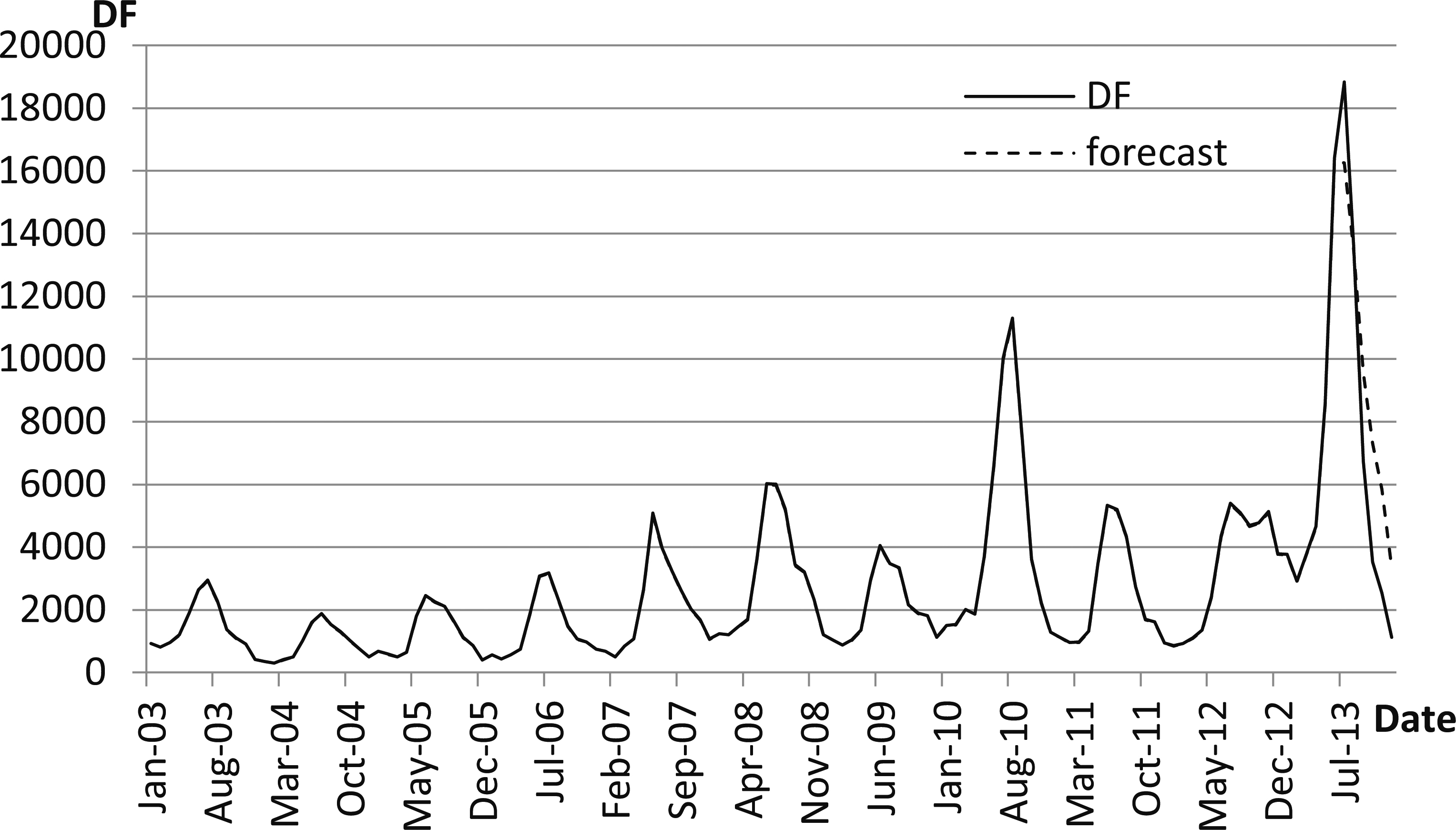

Figure 7.

Actual and forecasted values for AR(8)–ARCH(1) of the monthly number of DHF cases removed seasonal components from January 2003–December 2013.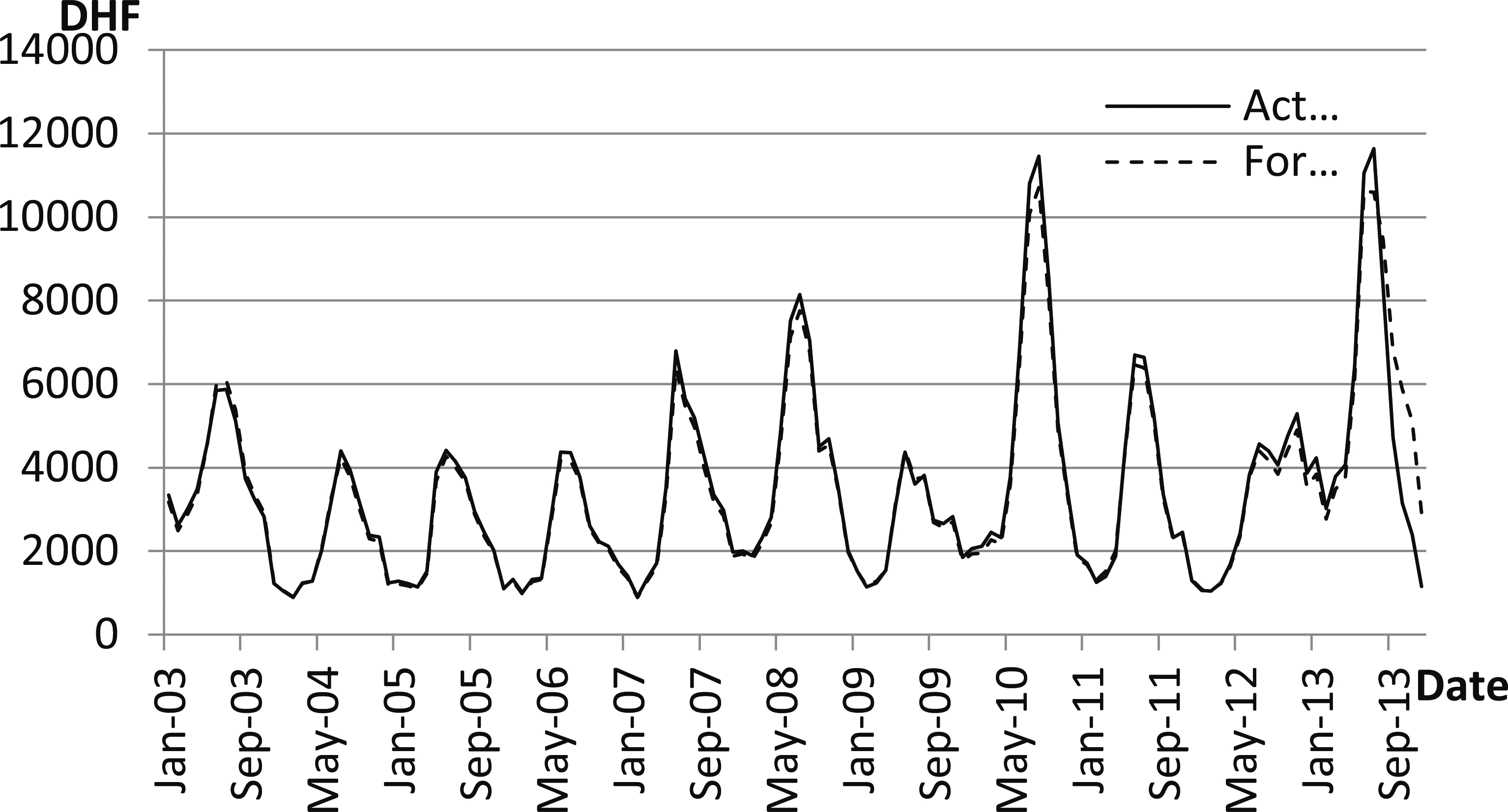

Figure 8.

Actual and forecasted values for AR(1)–ARCH(1) of the monthly number of DSS cases removed seasonal components from January 2003–December 2013.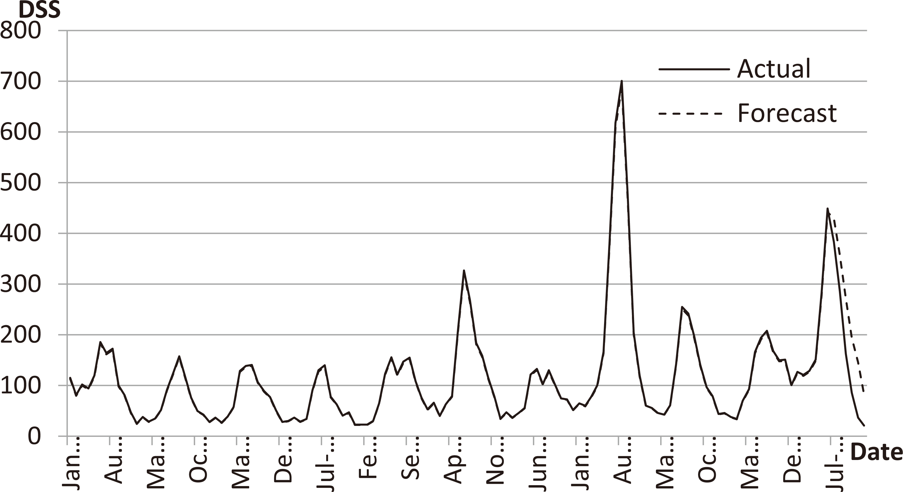

A GARCH model has the best fitting better than univariate Box-Jenkins models) to dengue because GARCH model comes with a variance equation that suitable for the data which its variance is depended on time like our data. It looks like GARCH method with a variance equation give a better fit than only transformation the data to make it stationary in variance before generate the model like the process of Box-Jenkins model do.

Moreover, the GARCH model with removing seasonal component is outperforming than the general GARCH model and the GARCH model adjusted by population size because our data also have an obviously seasonal effect but the GARCH model does not have a seasonal term. After we removed the seasonal components, the model has given a better fit to the data.

5. Forecasting

There are six models for each series. Hence we compare the results of the ARIMA and GARCH models with ensemble method (Sanchez, 2008; Suhartono, 2013). The results from either ensemble averaging or ensemble stacking methods are coincied with our best model in the previous section. Therefore, the DF, DHF, and DSS cases are forecasting using the best model which are shown in Figs 6–8, respectively.

6. Conclusion

This paper proposed the univariate Box-Jenkins (Seasonal ARIMA) model and the GARCH models to forecast dengue incidence in Thailand which consists of 3 types of syndromes i.e. dengue fever (DF), dengue hemorrhagic fever (DHF), and dengue shock syndrome (DSS). The GARCH model outperforms the seasonal ARIMA model for all 3 types of syndromes.

The best fitted model for DF, DHF and DSS are AR(1)–GARCH(1, 1), AR(8)–ARCH(1) and AR(1)–ARCH(1) removed the seasonal components, respectively. Along with, the percent errors of the best fitted models are 0.56%, 3.9% and 1.57%, respectively. In this study, the technique of adjustment by population size does not obviously improve model fitting and forecasting.

The population size may not be varied as much as expected. For the future work, we would like to apply the vector ARIMA model and the vector ARMA model removed the seasonal components to forecast dengue incidence in Thailand. Then compare them to the GARCH models. Further, the GARCH model is outperformed than either ARIMA or Seasonal ARIMA. But the GARCH model does not have the seasonal component it may be useful to propose GARCH model with taking into account of seasonal component in the GARCH model.

Footnotes

Acknowledgments

We would like to thank the Centre of Excellence in Mathematics, the Commission on Higher Education, Thailand, the Thailand Research Fund, and Mahidol University for the financial support.

References

Bhatnagar

Lal

Gupta

S. D.

, & Gupta

O. P.

(2012). Forecsting incidence of dengue in Rajasthan using time series analyses. Indian Journal of Public Health, 56(4), 281-285.

Bollerslev

(1986). Generalized autoregressive conditional heteroskedasticity. Journal of Econometrics, 31, 307-327.

Bureau of registration administration, Department of provincial administration, Ministry of Interior, (2014). The monthly number of population size in Thailand.

Bureau of the vector-borne diseases, Department of disease control, Ministry of public health, (2014). The monthly number of Dengue Fever, Dengue Hemorrhagic Fever and Dengue Shock Syndrome.

Catalano

, & Serxner

(1987). Time series designs of potential interest to epidemiologists. Am J Epidemiol, 26, 724-731.

Choudhury

M. A. H. Z.

Banu

, & Islam

A. M.

(2008). Forecasting dengue incidence in Dhaka, Bangladesh: A time series analysis. Dengue Bulletin, 32, 29-37.

Earnest

Chen

M. I.

Sin

L. Y.

(2005). Using autoregressive integrated moving average (ARIMA) models to predict and monitor the number of beds occupied during a SARS outbreak in a tertiary hospital in Singapore. BMC Health Serv Res, 5(1), 36.

Engle

R. F.

(1982). Autoregressive Conditional Heteroscedasticity with Estimates of the Variance of United Kingdom Inflation. The Econometrica, 50, 987-1007.

Donna

W. E.

(1995). An introduction to ARCH/GARCH Modeling using the AUTOREG Procedure. SAS Institute, WUSS95, 241-250.

10.

Gubler

D. J.

, & Kuno

(1997). Dengue and Dengue Hemorrhagic Fever. CAB International Wallingford UK, 1-22.

11.

Helfenstein

(1991). The use of transfer function models, intervention analysis and related time series methods in epidemiology. Int J Epidemiol, 20, 808-815.

12.

Kavinga

H. W. B.

Jayasundara

D. D. M.

, & Jayakody

D. N. K.

(2013). A new dengue outbreak statistical model using the time series analysis. European International Journal of Science and Technology, 2(10), 35-52.

13.

Kiatekarunya

(2011). Forecasting gold price in Thailand by using ARMA-GARCH. M Sc Thesis, Faculty of Economics, Chiang Mai University, Thailand.

14.

Liang

Hualiang

Linwei

Weizhong

Jimin

, & and Qiyong

(2009). Time series analysis of dengue fever and weather in Guangzhou, China. BMC Public Health, 9, 395.

15.

Martinez1

E. Z.

Silva

E. A. S.

, & Fabbro

A. L. D.

(2011). A SARIMA forecasting model to predict the number of cases of dengue in Campinas, State of São Paulo, Brazil. Revista da Sociedade Brasileira de Medicina Tropical, 44(4), 436-440.

16.

Nimmanpipaknit

(1997). Dengue hemorrhagic fever, Design CO., LTD, Bangkok, Thailand.

17.

Panthana

(1999). Four decades of dengue in Thailand. Pamphlet of Dengue, (2): 3.

18.

Paula

M. L.

Beatriz

V. M. M.

Claudia

T. C.

Claudio

J. S.

, & Alison

P. G.

(2008). Time Series analysis of dengue incidence in Rio de Janeiro, Brazil. The American Society of Tropical Medicine and Hygiene, 79(6), 933-939.

19.

Promprou

Jaroensutasinee

, & Jaroensutasinee

(2006). Forecasting Dengue Haemorrhagic Fever Cases in Southern Thailand using ARIMA Models. Dengue Bulletin, 30, 99-106.

20.

Pung

P. Y.

Miswan

N. H.

, & Ahmad

M. H.

(2013). Forecasting Malaysian gold using GARCH model. Applied Mathematical Sciences, 7(58), 2879-2884.

21.

Prajneshu

K. P. R.

, & Himadri

(2009). GARCH nonlinear time series analysis for modeling and forecasting of India’s volatile spices export data. Journal of the Indian Society of Agricultural Statistics, 63(2), 123-131.

22.

Reinaldo

C. G.

, & Javier

(2005). A GARCH forecasting model to predict day-ahead electricity prices. IEEE Transactions on Power Systems, 20(2), 867-874.

23.

Sanchez

(2008). Adaptive combination of forecasts with application to wind energy. International Journal of Forecasting, 24(4), 679-693.

24.

SAS Documentation. (2009). SAS/ETS

{}^{\@setsize{\tiny}{6pt}{\vpt}{\@vpt}\textregistered}

9.2 User’s Guide. SAS Institute Inc.

25.

Silawan

Singhasivanon

Kaewkungwal1

Nimmanitya

, & Suwonkerd

(2008). Temporal patterns and forecast of dengue infection in Northeastern Thailand. Southeast Asian J Trop Med Public Health, 39, 90-98.

26.

Siriwan

Mullica

, & (2012). Development of temporal modeling for prediction of dengue infection in Northeastern Thailand. Asian Pacific Journal of Tropical Medicine, 5(3), 249-252.

27.

Siti

R. Y.

Maizah

H. A.

Lee

C. N.

, & Noryanti

(2011). A comparative study on Box-Jenkins and GARCH models in forecasting crude oil prices. Journal of Applied Sciences, 11(7), 1129-1135.

28.

Suhartono

D. A. L.

(2013). Ensemble method based on two level ARIMAX-FFNN for rainfall forecasting in Indonesia. International Journal of Science and Research, 2(2), 144-149.

29.

Wei

W. W. S.

(2006). Time series analysis Univariate and multivariate methods. Second edition, Addison Wesley, USA.