Statistics-free sports prediction

Abstract

We use a simple machine learning model, logistically-weighted regularized linear least squares regression, in order to predict baseball, basketball, football, and hockey games. We do so using only the thirty-year record of which visiting teams played which home teams, on what date, and what the final score was. No real statistics are used, although a statistical method is used. The method works best in basketball, likely because it is high-scoring and has long seasons. It works better in football and hockey than in baseball, but in baseball the predictions are closer to a theoretical optimum. The football predictions, while good, can in principle be made much better, and the hockey predictions can be made somewhat better. These findings tells us that in basketball, most statistics are subsumed by the scores of the games, whereas in football, further study of game and player statistics is necessary to predict games as well as can be done. Baseball and hockey lie somewhere in between.

Keywords

Sports prediction ridge regression

1. Introduction

There is a long tradition in statistics in predicting many aspects of athletic events, in particular which teams will win, which players are the best, and the propensity of players to become injured. The tradition began in baseball, and was glorified in Moneyball (Lewis, 2004), but it has now extended to almost all other major sports. With the growing popularity of sports gambling and fantasy sites, there is more demand than ever for statistical information about which players will succeed and which teams will win.

This paper uses a simple, weighted, and penalized regression model (see Rifkin et al., 2003) to predict the outcome of MLB, NBA, NFL, and NHL games, using data going back more than thirty years scraped from the websites. It is similar to the model in Fearnhead and Taylor (2011), except it measures the ability of teams over games instead of players over possessions, and it does not take into account which team is at home. We intentionally limit our data use to the date, home and visiting teams, and score of each game, and we compare our predictions to a theoretically near-optimal indicator. Doing so tells us what statistical information is contained just in the scores, and whether what are commonly referred to as statistics have real predictive power. In basketball, the statistics are largely made unnecessary by the record of game scores, whereas in football this is clearly not the case. Baseball and hockey lie somewhere in the middle. This is likely because basketball has long seasons and high-scoring games, whereas baseball and hockey have long seasons but low-scoring games. Football has short seasons and is effectively low-scoring, because what matters is the number of scores that take place, not the scores’ point values. The models are trained on even-numbered years and tested on odd-numbered years.

The theoretically near-optimal indicator (which we also call the “oracle”) works as follows: Since our data is historical, we can predict every game by looking at the eventual end-of-season rankings and always bet that the eventually higher-ranked team will win. This estimator does not adjust for schedule difficulty, but is nonetheless very hard to beat. We demonstrate the performance of our penalized regression compared to this estimator. Furthermore, we show how it can be computed quickly using the Woodbury Matrix Identity.

We additionally prove that our model beats a straw man. To compute the straw man prediction of a game, look at the previous season’s ranking and predict that the higher ranking team will win. Our model almost always beats the straw man.

Table 1
Baseball predictions, MLB

Year of study	Methods	Source
1964	Formulas	(Cook, 1964)
1997	Markov process	(Bukiet, 1997)
2004	Bayesian hierarchical model	(Yang & Swartz, 2004)
2005	Regression	(Houser, 2005)
2005	Ensemble learning	(Lyle, 2007)
2006	Regression	(Abuaf et al., 2006)
2006	Regression	(Moy, 2006)
2009	Bayesian hierarchical model	(Jensen et al., 2009)
2009	Understanding winning streaks	(Sire & Redner, 2009)
2010	Bayesian hierarchical model	(Jiang & Zhang, 2010)
2014	k-nearest-neighbor	(Jang et al., 2014)

Table 2

Basketball predictions, NBA

Year of study	Methods	Source
1985	Hot Hand Effect	(Vallone & Tversky, 1985)
1994	Formulas	(Heit et al., 1994)
2004	Hot Hand Effect	(Caruso & Epley, 2004)
2011	Kalman filter	(Poropudas, 2011)
2012	Multiple methods	(Cao, 2012)
2013	k-means clustering	(Beckler et al., 2013)
2013	SVM/Ensemble methods/regression	(Cheng et al., 2013)
2013	logistic regression	(Clark et al., 2013)
2013	Genetic algorithm	(Puranmalka, 2013)
2013	Regression	(Summers, 2013)
2013	Regression	(Torres, 2013)
2015	Player position data	(Cervone et al., 2015)
2015	Regression	(Yang, 2015)
2016	Naive Bayes	(Wei, 2001)

Earnshaw Cook published the first major work on sabermetrics (baseball statistics) in 1964. Yang and Swartz (2004) use a Bayesian hierarchical model to predict Major League Baseball games, and Lyle (2007) does so using ensemble learning. Abuaf et al. (2006) and Moy (2006) predict baseball games using a number of statistics. Jang et al. (2014) uses a k-nearest-neighbor algorithm to predict Korean baseball games. Bukiet et al. (1997) model individual baseball games as Markov processes and studies many aspects of the game, including batting order, but does not post predictions. Sire and Redner (2009) study winning and losing streaks in baseball. Jensen et al. (2009) and Jiang and Zhang (2010) use Bayesian hierarchical models to study hitting performance in baseball. Houser (2005) believes the most important trait in a baseball player is his propensity to get on base. See Table 1.

The first model for predicting the outcome of professional basketball games appeared in Heit et al. (1994), which uses a formula to update a team’s strength after every game. Cervone et al. (2015) uses player position data to predict how likely an NBA team is to score on a given possession. Puranmalka (2013) uses a genetic algorithm, and achieves better results than we do in basketball prediction, but over a shorter time period, and only marginally so. Torres (2013) does about as well as we do at NBA prediction but also over a very short time span and using many statistics. These results do not contradict our thesis that the vast majority of the statistical power is contained simply in the scores of the games since their results are not that much better than ours. Beckler et al. (2013) and Yang (2015) use a simple models to predict NBA games, Poropudas (2011) uses a Kalman Filter, and Wei (2001) uses a Naive Bayes predictor. Cao (2012) surveys many NBA prediction methods. Cheng et al. (2013) predicts the betting line in NBA games. Clark et al. (2013) predict the likelihood of making a three-pointer using a logistic regression. Caruso and Epley (2004) and Vallone and Tversky (1985) study the hot hand effect, in which they do not believe. Summers (2013) studies how to win the playoffs. See Table 2.

Shi et al. (2013) use several machine learning methods, decision trees, rule learners, neural networks, naive Bayes, and random forests, and many statistics to predict NCAA basketball games. Brown and Sokol (2010), Carlin (1996), Caudill (2003), Stekler and Klein (2012) and Stoudt et al. use different methods to predict the NCAA men’s basketball. In fact, the Journal of Quantitative Analysis in Sports ran an entire issue on NCAA prediction in Glickman and Sonas (2015).

Table 3

Football predictions, NFL

Year of study	Methods	Source
1997	Probit regression	(DeJong, 1997)
1998	Bayesian hierarchical model	(Glickman & Stern, 1998)
2003	Neural network	(Kahn, 2003)
2003	Studies the draft	(McGee & Burkett, 2003)
2010	Bayesian hierarchical model	(Warner, 2010)
2011	Neural networks	(Blaikie et al., 2011)
2012	Plotting	(Szalkowski & Nelson, 2012)
2013	Logistic regression	(Warner, 2010)
2014	Multiple methods	(Balreira, 2014)

Table 4

Hockey predictions, NHL

Year of study	Methods	Source
2011	Bayesian hierarchical model	(Buttrey et al., 2011)
2011	Bayesian hierarchical model	(Leard & Doyle, 2011)
2014	Neural networks	(Weissbock, 2014)
2014	Multiple machine learning models	(Weissbock & Inkpen, 2014)

DeJong (1997) uses a probit regression to predict football games, and Kahn (2003) uses a neural network to predict football games. Glickman and Stern (1998) use a Bayesian hierarchical model to predict football games. Balreira et al. (2014) use numerous methods to predict NFL games. West and Lamsal (2008) predict college football games. Blaikie et al. (2011) use neural networks to predict both professional and college football games. Harville (1977) uses a stochastic process model to rate high school and college football teams.

Szalkowski and Nelson (2012) explain the extent to which casino betting lines predict NFL games, which raises interesting questions about the power of democracy in prediction. Warner (2010) predicts the betting lines. Sinha et al. (2013) predicts NFL games using Twitter, another democratic approach. McGee and Burkett (2003) study the NFL draft. See Table 3.

There is also some past work done on NHL hockey, including one paper on game prediction (Weissbock, 2014) using neural networks, and one paper on scoring rates (Buttrey et al., 2011). There are other papers using various factors to predict hockey games (Leard & Doyle, 2011; Weissbock & Inkpen, 2014). See Table 4.

Blundell (2009) and Haghighat et al. (2013) survey a group of machine learning methods used in sports prediction in general. There is also a wealth of research on the statistics of soccer games.

In the next section we describe a model that takes scores from historical games and predicts the winner of future games. We then evaluate its performance on historical data.

2. The model

The general scheme is to put the scores of the games in a vector, $b$ , and say that a score in $b$ is the sum of an offensive parameter and a defensive parameter both in $x$ . The matrix $A$ has $1$ ’s and $0$ ’s indicating which teams played in the game, so $b\sim Ax$ . Furthermore, $x$ has an $L_{2}$ (ridge) penalty to apply Occam’s Razor. $A$ and $b$ are weighted by a matrix $D$ that uses a logistic function to weight recent games more highly and less recent games less so.

For $y$ denoting the year, let $b^{(y)}$ be a vector such that $b^{(y)}_{2i-1:2i}$ are the visiting and home scores, respectively, in the $i$ -th game of the year $y$ season. $b^{(y)}_{2i-1}$ is the home score and $b^{(y)}_{2i}$ is the visiting score. Let $L^{(y)}$ be twice the number of games in year $y$ and let $P$ be the total number of teams that have played in either the MLB, NBA, NFL, or NHL since the 1986 season. Let $A^{(y)}$ be an $L^{(y)}\times 4P$ matrix that is all zeros except that if teams $j$ and $k$ are the visitors and home teams in game $i$ of the year $y$ season, $A^{(y)}_{2i-1,j}=A^{(y)}_{2i-1,k+P}=A^{(y)}_{2i,k+2P}=A^{(y)}_{2i,j+3P}=1$ . The four $1$ ’s pluck the weights in $w$ corresponding to which team is visiting and which team is home in game $i$ and compare them linearly to predict the score of the match, i.e. $b$ is regressed on $A$ with ridge penalty and with coefficients in $w$ . The regression errors are weighted by a matrix $D$ , which makes recent games count more, as we shall see. Setting up the $A^{(y)}$ matrices in this way allows the model to take home-field advantage into account. Let $y_{\rm back}$ be the number of seasons considered other than the current season used to predict the current season, it is sport-dependent. In baseball, football, and hockey $y_{\rm back}=4$ , and in basketball $y_{\rm back}=2$ .

Table 5
Model predictions compared

	Model	Oracle	Straw man
MLB Even Years 1986–2015	0.5524	0.5756	0.5370
MLB Odd Years 1986–2015	0.5480	0.5760	0.5317
MLB All Years 1986–2015	0.5502	0.5758	0.5301
NBA Even Years 1986–2015	0.6869	0.6840	0.6229
NBA Odd Years 1986–2015	0.6773	0.6812	0.6144
NBA All Years 1986–2015	0.6821	0.6826	0.6187
NFL Even Years 1986–2015	0.6347	0.7184	0.5859
NFL Odd Years 1986–2015	0.6241	0.7188	0.5749
NFL All Years 1986–2015	0.6294	0.7186	0.5823
NHL Even Years 1986–2015	0.5821	0.6093	0.5588
NHL Odd Years 1986–2015	0.5897	0.6125	0.5650
NHL All Years 1986–2015	0.5918	0.6136	0.5666

Figure 1.

MLB: Our model (middle) vs. the oracle (top) and the straw man (bottom).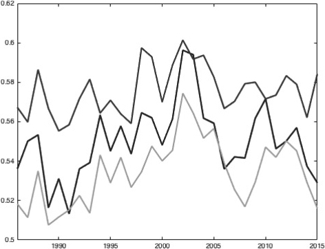

Figure 2.

NBA: Our model (middle, darkest) vs. the oracle (top) and the straw man (bottom).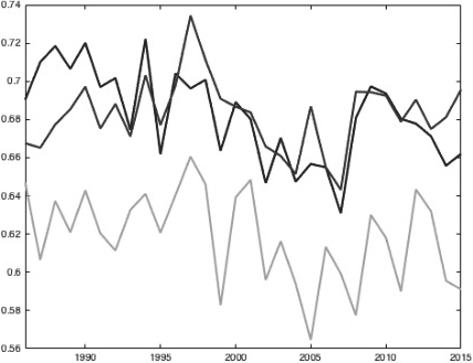

Let $D^{(z)}$ be a diagonal matrix such that

$D^{(z)}_{l,l}=d_{1}^{(z)}+\frac{d_{2}^{(z)}}{1+\exp\left(-d_{3}^{(z)}\left(% \frac{l}{L^{(z)}}-d_{4}^{(z)}\right)\right)},$

where the $d^{(z)}_{1:4}$ are tuning parameters picked by maximizing the predictivity of the upcoming model on even-numbered years. The even-numbered years are our training set and the odd-numbered years are our test set. We pick the logistic curve because of its versatility; it can model a line, a concave-up curve, a concave-down curve, and a step function. It is used to weight games that occured more recently more highly in finding the weights in $b^{(y)}$ .

For matrices $U^{(1)},\ldots,U^{(n)}$ , let their vertical concatenation be

$[U^{(1)};\ldots;U^{(n-1)};U^{(n)}],$

with $U^{(1)}$ on top. We will now explain how to predict whether $b^{(y)}_{2i-1}-b^{(y)}_{2i}$ is positive or negative using only historical data (If it is zero we say that we predicted it correctly one half of one time. Since this is not a win and not a loss we think this is an appropriate bookkeeping convention). $b^{(y)}_{2i-1}-b^{(y)}_{2i}$ is the difference in scores between the visiting team and the home team, so if it is positive, the visiting team wins, if it is negative, the home team wins, and if it is zero, it is a tie. We use a weighted regularized linear least squares regression, information about them can be found in Rifkin et al. (2003). Let

$\displaystyle X^{(y)}=[D^{(y_{\rm back})}A^{(y-y_{b})};\ldots;D^{(1)}A^{(y-1)}% ;D^{(0)}A^{(y)}],$ $\displaystyle Y^{(y)}=[D^{(y_{\rm back})}b^{(y-y_{b})};\ldots;D^{(1)}b^{(y-1)}% ;D^{(0)}b^{(y)}],$

and let $M^{(y)}=L^{(y-y_{\rm back})}+\ldots+L^{(y-1)}+L^{(y)}$ . Let

$\displaystyle K^{(y,i)}=\left(X^{(y)}_{1:(M^{(y)}+2i-2),:}\right)^{t}X^{(y)}_{% 1:(M^{(y)}+2i-2)},$ $\displaystyle w^{(y,i)}=\left(K^{(y,i)}+I\right)^{-1}\left(X^{(y)}_{1:(M^{(y)}% +2i-2),:}\right)^{t}Y^{(y)}_{1:(M^{(y)})+2i-2}.$

Typically there is a positive $\lambda$ parameter in front of the $I$ , we omit it for itis absorbed by the $D^{(z)}$ . Typically also $X^{(y)}$ and $Y^{(y)}$ would be centered. Empirically this appears unnecessary for our problem. It is not necessary to invert the whole matrix, Gaussian elimination may be used. To do prediction, set

$\hat{Y}^{(y)}_{(M^{(y)}+2i-1):(M^{(y)}+2i)}=X^{(y)}_{(M^{(y)}+2i-1):(M^{(y)}+2% i),:}w^{(y,i)}.$

The sign of $\hat{Y}^{(y)}_{M^{(y)}+2i-1}-\hat{Y}^{(y)}_{M^{(y)}+2i}$ predicts the sign of $b^{(y)}_{2i-1}-b^{(y)}_{2i}$ , in other words, which team will win. Remember, the teams playing are contained in rows $(M^{(y)}+2i-1):(M^{(y)}+2i)$ of $X^{(y)}$ . The entries in the $D^{(z)}$ are picked so that the sum of the model’s correct predictions is as high as possible on even years.

This process can be accelerated. First compute

$\displaystyle K^{(y,1)}=\left(X^{(y)}_{1:M^{(y)},:}\right)^{t}X^{(y)}_{1:M^{(y% )},:},$ $\displaystyle w^{(y,1)}=\left(K^{(y,1)}+I\right)^{-1}\left(X^{(y)}_{1:M^{(y)},% :}\right)^{t}Y^{(y)}_{1:M^{(y)}}.$

Hypothesize that we know $K^{(y,i)}$ and $w^{(y,i)}$ , we will find them for $i+1$ . Let $\tilde{x}=X^{(y)}_{(M^{(y)}+2i-3):(M^{(y)}+2i-2)}$ , $\tilde{y}=Y^{(y)}_{(M^{(y)}+2i-3):(M^{(y)}+2i-2)}$ , and $\tilde{u}=(K^{(y,i)}+I)^{-1}\tilde{x}^{t}$ . By the Woodbury Matrix Identity,

$\displaystyle w^{(y,i+1)}=(I-\tilde{u}(I_{2\times 2}+\tilde{x}\tilde{u})^{-1}% \tilde{x})(\tilde{w}+\tilde{u}\tilde{y}),$ $\displaystyle K^{(y,i+1)}=K^{(y,i)}+\tilde{x}^{t}\tilde{x}.$

3. Results

Figure 3.

NFL: Our model (middle) vs. the oracle (top) and the straw man (bottom).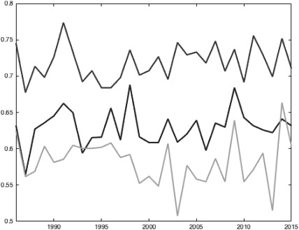

Figure 4.

NHL: Our model (middle) vs. the oracle (top) and the straw man (bottom). Note that the 2005 season was unfinished due to a strike.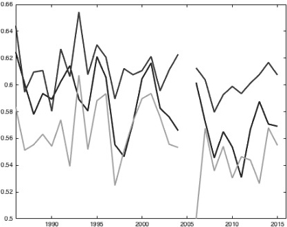

Figure 5.

NBA: Teams are located on the x-axis (the best on a left); y-axis shows a percentage of the really won (descending) and predicted by our model (jagged) games in 2015 season.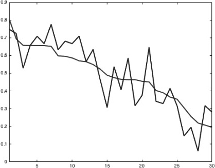

All computations were done using Matlab.

Table 5 shows the results of the model on all four sports, on the even years on which it was trained, on the odd years, and on all years. The form of the results is the probability of correctly predicting the winner of a game. The Model column denotes the performance of our model, whereas the Oracle column denotes the performance of the theoretically hard-to-beat model described in the introduction which uses information from the future to predict the past. The Straw Man was described in the introduction.

To reiterate, the theoretically near-optimal indicator works as follows: Since our data is historical, we can predict every game by looking at the eventual end-of-season rankings and always bet that the eventually higher-ranked team will win. This estimator does not adjust for schedule difficulty, but is nonetheless very hard to beat.

The even numbered years are our training set and the odd numbered years are our test set. Note that hte training and test set performance are similar.

The first four figures (Figs 1–4) show the performance of our model (in blue) vs. the oracle (in red) and the straw man (in green) in every year from 1986–2015. The performance is measured by the ratio of games predicted correctly. The figures are in the order MLB, NBA, NFL, NHL. They show that the model performs well in basketball, which has long seasons and high-scoring games. It performs passably in baseball and hockey and poorly in football. These results indicate that most basketball statistics are subsumed by the game scores. This is somewhat the case in baseball and hockey and not the case in football. The hockey graph jumps during the strike in the 2005 season.

Figure 5 compares actual and model-predicted wins for the NBA. Expectedly, the NBA graph shows the model to be accurate.

4. Conclusion

We see that the basketball predictor comes very close to and sometimes outperforms the oracle, even though it only uses game scores. The theoretically near-optimal indicator (which we also call the “oracle”) works as follows: Since our data is historical, we can predict every game by looking at the eventual end-of-season rankings and always bet that the eventually higher-ranked team will win. This fact suggests that adding more traditional statistics probably has limited value for predicting NBA matches. Furthermore, this fact is predictable. Basketball games are high scoring, so by the law of averages the better teams usually win. Furthermore, basketball has long seasons, so it is easy to identify which teams are better and best. Other sports are less like basketball because they do not have these properties. Baseball and hockey have long seasons but are low scoring. Football is higher-scoring but has short seasons. More work is necessary in predicting baseball, football, and hockey more optimally.

Footnotes

Acknowledgments

The author thanks the anonymous referees for their helpful comments.

References

http://www.baseball-reference.com.

http://www.basketball-reference.com.

http://www.pro-football-reference.com.

http://www.hockey-reference.com.

Abuaf

Chen

, & Trifunac

(2006). Can One Predict Next Year’s Winning Percentage using OLS Regression on Baseball Statistics? available online.

Balreira

E. C.

Miceli

B. K.

, & Tegtmeyer

(2014). An oracle method to predict NFL games. Journal of Quantitative Analysis in Sports, 10, 183-196.

Beckler

Wang

, & Papamichael

(2013). NBA Oracle, available online.

Blaikie

A. D.

Abud

G. J.

David

J. A.

, & Pasteur

R. D.

(2011). NFL & NCAA Football Prediction using Artificial Neural Networks. Proceedings of the 2011 Midstates Conference on Undergraduate Research in Computer Science and Mathematics.

Blundell

J. D.

(2009). Numerical Algorithms for Predicting Sports Results, available online.

10.

Brown

, & Sokol

(2010). An Improved LRMC Method for NCAA Basketball Prediction. J Quant Anal Sports, 6(3), Article 4.

11.

Bukiet

Harold

E. R.

, & Palacios

J. L.

(1997). A Markov Chain Approach to Baseball. Operations Research, 45(1), 14-23.

12.

Buttrey

S. E.

Washburn

A. R.

, & Price

W. L.

(2011). Estimating NHL Scoring Rates. Journal of Quantitative Analysis in Sports, 7(3).

13.

Cao

(2012). Sports Data Mining Technology Used in Basketball Outcome Prediction. Master’s Dissertation, Dublin Institute of Technology.

14.

Carlin

B. P.

(1996). Improved NCAA basketball tournament modeling via point spread and team strength information. The American Statistician, 50(1), 39-43.

15.

Caruso

E. M.

, & Epley

(2004). Hot hands and cool machines: Perceived intentionality in the prediction of streaks, available online.

16.

Caudill

S. B.

(2003). Predicting discrete outcomes with the maximum score estimator: The case of the NCAA men’s basketball tournament. International Journal of Forecasting, 19, 313-317.

17.

Cervone

D’Amour

Bornn

, & Goldsberry

(2015). A Multiresolution Stochastic Process Model for Predicting Basketball Possession Outcomes, arXiv.

18.

Cheng

Dade

Lipman

, & Mills

(2013). Predicting the Betting Line in NBA Games, available online.

19.

Clark

T. K.

Johnson

A. W.

, & Stimpson

A. J.

(2013). Going for three: Predicting the likelihood of field goal success with logistic regression. 7-th annual MIT Sloan Sports Analytics Conference.

20.

Cook

(1964). Percentage Baseball. Waverly Press.

21.

DeJong

D. N.

(1997). Using past performance to predict NFL outcomes: A chartist approach, available online.

22.

Fearnhead

, & Taylor

B. M.

(2011). On estimating the ability of NBA players. Journal of Quantitative Analysis in Sports, 47(3), 1298.

23.

Vallone

, & Tversky

(1985). The hot hand in basketball: On the misperception of random sequences. Cognitive Psychology, 17, 295-314.

24.

Glickman

M. E.

, & Stern

H. S.

(1998). A state-space model for national football league scores. Journal of the American Statistical Association, 93(441).

25.

Glickman

M. E.

, & Sonas

(2015). Introduction to the NCAA men’s basketball prediction methods issue. J Quant Anal Sports, 11(1), 1-3.

26.

Haghighat

Rastegari

, & Nourafza

(2013). A review of data mining techniques for result prediction in sports. ACSIJ, 2(5), 6.

27.

Harville

(1977). The use of linear-model methodology to rate high school or college football teams. Journal of the American Statistical Association, 72(358), 278-289.

28.

Heit

Price

P. C.

, & Bower

G. H.

(1994). A model for predicting the outcomes of basketball games. Applied Cognitive Psychology, 8, 621-639.

29.

Houser

(2005). Which baseball statistic is the most important when determining team success? The Park Place Economist, Volume XIII.

30.

Jang

Nasridinov

, & Park

(2014). Analyzing and predicting patterns in baseball data using machine learning techniques. Advanced Science and Technology Letters, 62, 37-40.

31.

Jensen

S. T.

McShane

B. B.

, & Wyner

A. J.

(2009). Hierarchical Bayesian modeling of hitting performance in baseball. Bayesian Analysis.

32.

Jiang

, & Zhang

(2010). Empirical Bayes in-season prediction of baseball batting averages. 6, 263-273.

33.

Kahn

(2003). Neural Network Prediction of NFL Football Games, available online.

34.

Leard

, & Doyle

J. M.

(2011). The effect of home advantage, momentum, and fighting on winning in the national hockey league. Journal of Sports Economics, 12(5), 538-560.

35.

Lewis

(2004). Moneyball: The Art of Winning an Unfair Game. W W Norton & Company, New York, NY.

36.

Lyle

(2007). Baseball Prediction Using Ensemble Learning, available online.

37.

McGee

K. J.

, & Burkett

L. N.

(2003). The national football league combine: A reliable predictor of draft status? Journal of Strength and Conditioning Research, 17(1), 6-11.

38.

Moy

(2006). Regression Planes to Improve the Pythagorean Percentage: A regression model using common baseball statistics to project offensive and defensive efficiency, Undergraduate Thesis, U.C. Berkeley.

39.

Poropudas

(2011). Kalman Filter Algorithm for Rating and Prediction in Basketball, Master’s Thesis, University of Helsinki, Faculty of Social Sciences.

40.

Puranmalka

(2013). Modelling the NBA to Make Better Predictions, Master’s Thesis, MIT.

41.

Rifkin

Yeo

, & Poggio

(2003). Book chapter, Regularized Least-Squares Classification. http://cbcl.mit.edu/publications/ps/rlsc.pdf.

42.

Shi

Moorthy

, & Zimmerman

(2013). Predicting NCAAB match outcomes using ML techniques – some results and lessons learned, arXiv.

43.

Sinha

Dyer

Gimpel

, & Smith

N. A.

(2013). Predicting the NFL Using Twitter, arXiv.

44.

Sire

, & Redner

(2009). Understanding baseball team standings and streaks. Eur Phys J B, 67, 473-481.

45.

Stekler

H. O.

, & Klein

(2012). Predicting the outcomes of NCAA basketball championship game. Research Program on Forecasting, Working Paper No. 2011-003.

46.

Stoudt

Santana

, & Baumer

In Pursuit of Perfection: An Ensemble Method for Predicting March Madness Match-Up Probabilities, available online.

47.

Summers

M. R.

(2013). How to Win in the NBA Playoffs: A Statistical Analysis. American Journal of Management, 13(3).

48.

Szalkowski

, & Nelson

M. L.

(2012). The Performance of Betting Lines for Predicting the Outcome of NFL Games, arXiv.

49.

Torres

R. A.

(2013). Prediction of NBA games based on Machine Learning Methods, available on the internet.

50.

Warner

(2010). Predicting Margin of Victory in NFL Games: Machine Learning vs. the Las Vegas Line, available on the internet.

51.

Wei

(2001). Predicting the outcome of NBA playoffs using the Naive Bayes Algorithms, available on the internet.

52.

Weissbock

(2014). Forecasting Success in the National Hockey League using In-Game Statistics and Textual Data, Master’s Thesis, University of Ottawa.

53.

Weissbock

, & Inkpen

(2014). Combining Textual Pre-game Reports and Statistical Data for Predicting Success in the National Hockey League, Advances in Artificial Intelligence. Volume 8436 of the series Lecture Notes in Computer Science, pp. 251-262.

54.

West

B. T.

, & Lamsal

(2008). A new application of linear modeling in the prediction of college football bowl outcomes and the development of team ratings. J Quant Anal Sports, 4(3), Article 3.

55.

Yang

T. Y.

, & Swartz

(2004). A two-stage Bayesian model for predicting winners in major league baseball. Journal of Data Science, 2, 61-73.

56.