The ensemble of neural network and gradient boosting for the prediction of customer profitability: A two-stage modeling approach

Abstract

This paper illustrates a two-stage approach for predicting customer profitability. The first stage is to build a dichotomous model to predict the customer’s likelihood of future purchase. The second stage is to build a model, with continuous target variable, to predict the conditional future profit generated by the customer given he would make a purchase. Both stages involve the utilization of the gradient boosting and neural network data-mining techniques. In each stage, various ensemble combinations are tried and the one resulting in the lowest validation average squared error is chosen to be the stage model winner. The two model winners are subsequently used jointly for the prediction of future profit. In this analysis, Base SAS ${}^{\@setsize{\tiny}{6pt}{\vpt}{\@vpt}\textregistered}$ is used for data manipulation and SAS ${}^{\@setsize{\tiny}{6pt}{\vpt}{\@vpt}\textregistered}$ Enterprise Miner™ 13.2 is used for predictive modeling. It is evident that this two-stage modeling approach is robust in predicting customer profitability. Managerial and research implications will be highlighted.

Keywords

Customer profitability prediction of future profit non-contractual product purchases two-stage model data-mining ensemble

1. Introduction

Customer value, or customer lifetime value (CLTV) in the longer-term perspective, has been a well-researched area in both academia and commercial domains (EsmaeiliGookeh & Tarokh, 2013; Damn & Monroy, 2011; Singh & Jain, 2010; Malthouse & Blattberg, 2005). It is an important topic in customer relationship management, and was defined by Kotler as the present value of the future profit stream expected given a time horizon of transacting with the customer (Kotler, 1974). One primary goal in the context of customer lifetime value is to understand how one customer differs from another. In fact, it is generally believed that a small percentage of customers account for a large percentage of revenue and profit (Mulhern, 1999), thus implying that the distribution of customer value is somewhat skewed. This phenomenon is also consistent to the Pareto Principle (Vilfredo Pareto 1848–1823) which states that for many phenomena, about 80% of the consequences are produced by 20% of the causes (Dunford et al., 2014). The same phenomenon can further be illustrated by considering Formula 1 – a formula commonly used (the interest rate factor is neglected) for calculating customer lifetime value (CLTV).

$\displaystyle\textit{CLTV}=\mathop{\sum}\limits_{t=1}^{K}P_{t}\cdot M_{t}$ (1)

The formula assumes that the time horizon is divided into $K$ consecutive periods, where $P_{t}$ is the predicted probability that a customer will remain being a customer or make a purchase at the $t^{\text{th}}$ period, and $M_{t}$ is the predicted conditional future profit during the $t^{\text{th}}$ period. When a customer became inactive or made no purchase at the $t^{\text{th}}$ period, he would generate zero profit. In reality, a business operation may have many in-frequent or one-time off customers. They are those who make only one lifetime purchase and thereafter make zero purchase (Erdman et al., 2008; Kapitula, 2015) in the subsequent measurement period(s). When an analyst includes them in the analysis, he would find the empirical customer value distribution to be (highly) skewed, and this would require some adjustment in the modeling. From the business perspective, marketing managers may also want to find ways to identify them (Liu et al., 2016) from the customer portfolio for appropriate customer re-engagement targeting. To the end of these, the prediction of $P_{t}$ would become most important.

The approach for estimating $P_{t}$ varies by industries or nature of the product (Fader & Hardie, 2009). For industries like telecommunications, insurance or country club in which product purchase is usually not a repeated event and mostly contractual in nature, researchers often analyze the length of time (i.e. till the $t^{\text{th}}$ period) it takes for the customer to churn (Pliner, 2016; Lu, 2003; Thatt & Chakraborty, 2015). Modeling techniques such as proportional hazard model and discrete time hazard model are commonly employed for this. For industries like retailing, hospitality or doctor visits in which product purchase is often repetitive and non-contractual in nature, researchers usually examine which of the $K$ periods the customer would make a purchase (Lund, 2015; Lund, 2016). Multinomial logistic model is often used in this context, and some researchers also use probabilistic/stochastic models (Pfeifer & Carraway, 2000; Fader & Hardie, 2009). For estimating $M_{t}$ , regression based approaches such as generalized linear models are commonly used.

This research focuses on non-contractual product purchases. Instead of considering the entire lifetime horizon, this analysis will focus on predicting the two quantities and the customer value in a shorter time-period (i.e. $P_{1}$ and $M_{1}$ ), given by

$\displaystyle\text{Customer Value}=P_{1}\cdot M_{1}$ (2)

In fact, Eq. (2) could be re-written as

$\displaystyle\text{Customer Value}=P_{1}\cdot M_{1}+(1-P_{1})\cdot 0$ (3)

Equation (3) essentially represents a two-part or two-stage model (Kapitula, 2015), including two components – the purchaser and non-purchaser population. The second term means that if a customer is predicted to be a non-purchaser ( $1-P_{1}$ ) in the upcoming period (first period), a conditional profit of zero is to be assigned. This two-stage model could be built using the finite mixture modeling approach via the PROC FMM or NLMIXED procedure (Kessie & McDowell, 2012; Huang & Xie, 2012). This paper attempts to demonstrate the construction of a two-stage prediction model from scratch. In each stage, the neural network and gradient boosting data-mining techniques as well as their ensemble models will be constructed. The advantage is that the same methodological framework can be extended to encompass other mix of data-mining techniques as well as to account for a wider time horizon, for a fuller prediction of longer-term customer lifetime value.

Figure 1.

A two-stage modeling framework for the prediction of future profit.

2. Methodology

Profit is taken as a proxy of customer value. This study attempts to predict the future profit generated by existing customers. An existing customer is defined as someone who has prior purchase experience. He could be someone who made his first purchase yesterday; or someone who made his first purchase 3 years ago and thereafter placed a few orders in each subsequent year; or someone who bought 2 years ago but since then has made no more purchase as of today. The profit is defined as the gross profit margin (i.e. sales minus cost-of-good-sold), and we want to predict the profit an existing customer would generate for the company in the next 12 months. A period of 12-month is chosen simply because it covers all business seasons of a full financial year, and the model prediction as such derived would organically exempt from the influence of seasonality, in regardless of the starting month of any 12-month horizon.

Figure 2.

The base and prediction period.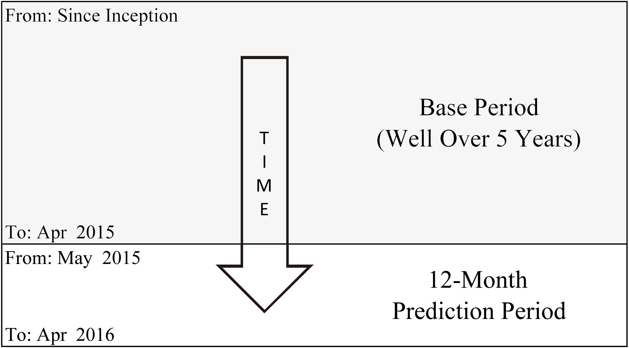

2.1 The two-stage modeling framework

Refer to Fig. 1. Two models are built. Model 1 predicts how likely (i.e. probability $=P$ ) an existing customer would make a purchase (i.e. at least one purchase) in the next 12 months. Model 2 predicts the conditional future profit given the customer would make a purchase. The two predictions are used jointly (i.e. adjustment of non-purchaser selection bias) to produce the expected future profit – the (unconditional) predicted future profit.

2.2 Sampling

The dataset utilized in this analysis is originated from an anonymous business operation which delivers consumable products to the general consumer market. For confidentiality reason, all the variable names, figures and profitability results are masked. We bookmark the status (e.g. prior usage behavior and loyalty membership status) of the existing customers as of the last day of April2015 (the reference date), and then predict as well as observe their actual purchase behavior (i.e. whether they purchase or not, and the associated profit margins) in the next 12 months (May 2015 to April 2016). A pictorial representation is shown in Fig. 2.

Table 1
Sampling summary

Event	Sample	Model 1	Model 2	Testing	Not used
Purchase	37,877	22,500	22,500	15,377
	21.0%	50.0%	100.0%	21.0%
Not purchase	142,123	22,500		57,698	61,925
	79.0%	50.0%		79.0%
Total	180,000	45,000	22,500	73,075	61,925

Table 2

Variable descriptions

Target
	Purchase (Binary/1-Purchase & 0-Not Purchase, in the prediction period)
	Profit (Numeric/Gross profit margin in dollars, in the prediction period)
Acquisition Order
	First_Quantity (Numeric/The quantity of items purchased in the first order)
	First_Spending (Numeric/The dollars spending in the first order)
Individual Usage
	Lifetime_Recency (Numeric/The lifetime purchase recency of the customer as of the end of the base period)
	Lifetime_Frequency (Numeric/The lifetime number of purchases of the customer as of the end of the base period)
	Lifetime_Spending (Numeric/The lifetime dollars spending of the customer as of the end of the base period)
	Frequency_0_1Yr (Numeric/The number of purchases of the customer in the most recent 1 year)
	Frequency_1_2Yr (Numeric/The number of purchases of the customer in the year prior to the most recent 1 year)
	Spending_0_1Yr (Numeric/The dollars spending of the customer in the most recent 1 year)
	Spending_1_2Yr (Numeric The dollars spending of the customer in the year prior to the most recent 1 year)
Zip-Based Usage
	Zip_Lifetime_Recency (Numeric/The zipcode based recency)
	Zip_Lifetime_Frequency (Numeric/The zipcode based total number of purchases)
	Zip_Lifetime_Spending (Numeric/The zipcode based total dollars spending)
Third Party
	Third_Binary_V1 – Third_Binary_V4 (Four anonymous third-party binary variables)
	Third_Integer_V5 – Third_Integer_V9 (Five anonymous third-party integer variables)
	Third_Numeric_V10 – Third_Numeric_V17 (Eight anonymous third party numeric variables)
Miscellaneous
	Email_Availability (Binary/1-the customer has an email for marketing communications, and 0 otherwise)
	Loyalty_Status (Binary/1-the customer is a loyalty member, and 0 otherwise)
	Store_Proximity (Numeric/The customer’s residential locational distance from the closest store, in miles)
	Tenure (Numeric/The number of days lapsed since the first purchase)

Remark: The status of all input variables is measured based on the reference date of 30 Apr 2015.

See Table 1, a total of 180,000 existing customers (who bought at least once during the base period) are randomly selected from the company database. This sample records a “Purchase” to “Not Purchase” ratio of 21.0% to 79.0% in the prediction period. A total of 22,500 customers are randomly drawn from the “Purchase” group without replacement. These 22,500 customers are combined with another 22,500 random observations drawn from the “Not Purchase” group (again without replacement) to form the modeling dataset for building Model 1, and the same 22,500 customers from the “Purchase” group is used to build Model 2. For the remaining 15,377 observations from the “Purchase” group, they are combined with 57,698 random observations drawn from the balance (i.e. 142,123 – 22,500 $=$ 119,623) of the “Not Purchase” group to form a test dataset: TEST_DATASET. This test dataset, which is purposely assembled to obtain the same “Purchase” to “Not Purchase” ratio as that of the whole sample, will be used for the final validation.

Figure 3.

Profit distribution (full sample).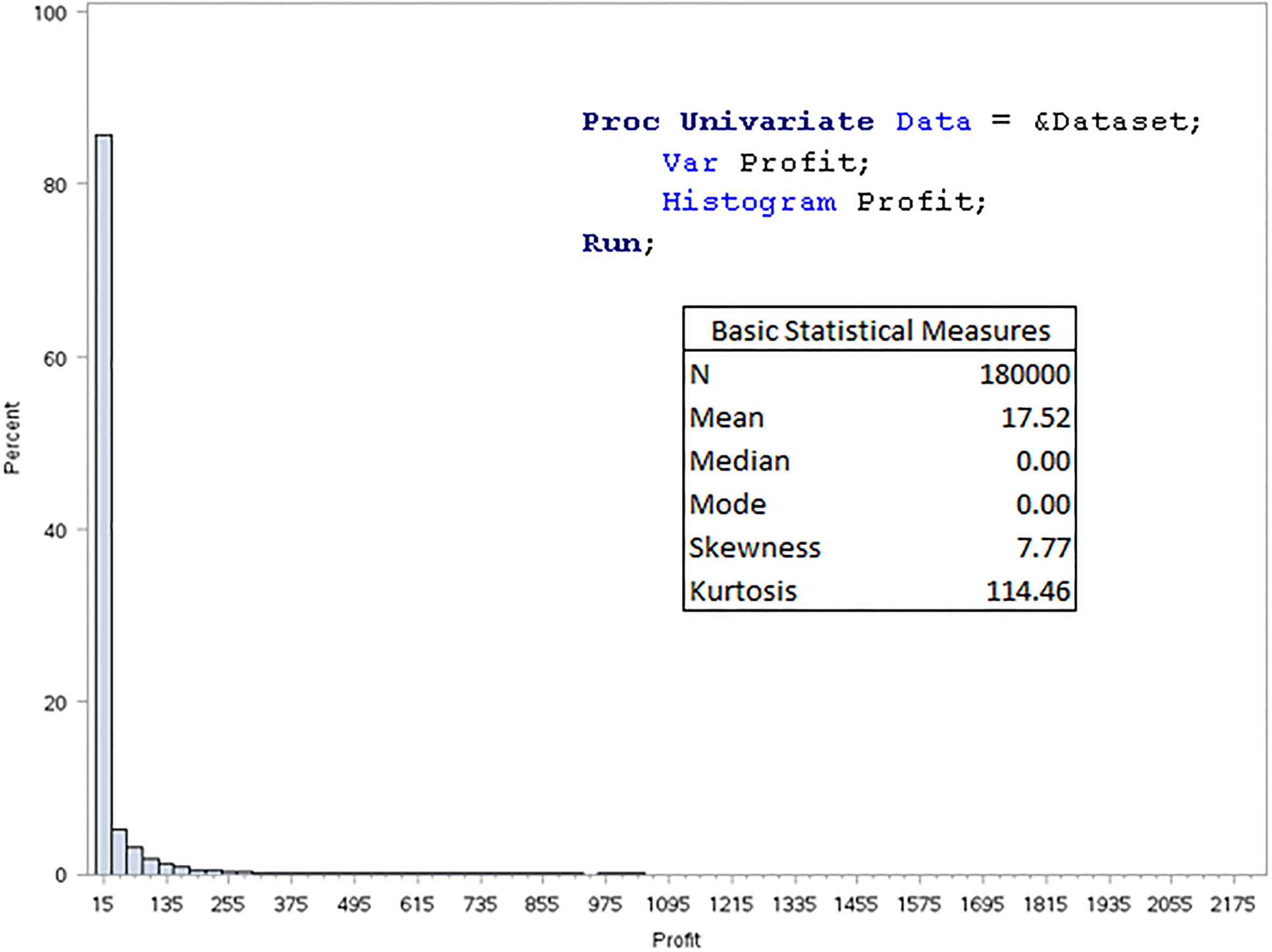

2.3 Data descriptions

All the target and input variables used in this study are summarized in Table 2.

3. Model building

3.1 Exploratory analysis

One important practice in any predictive modeling project is to obtain an initial picture of the distribution of the target variable. This can be achieved through a Proc Univariate routine. The results of such routine reveal (see Fig. 3) that the target: Profit is highly skewed. Both the skewness and kurtosis are far from zero; and the location measure mean (17.5) and median (0.0) do not align. This is not unexpected since we know from Table 1 that 79.0% of the sampled customers have not made any purchase in the prediction period. Nevertheless, such highly skewed target distribution may pose difficulty in predictive modeling.

Figure 4.

Profit distribution (purchaser only).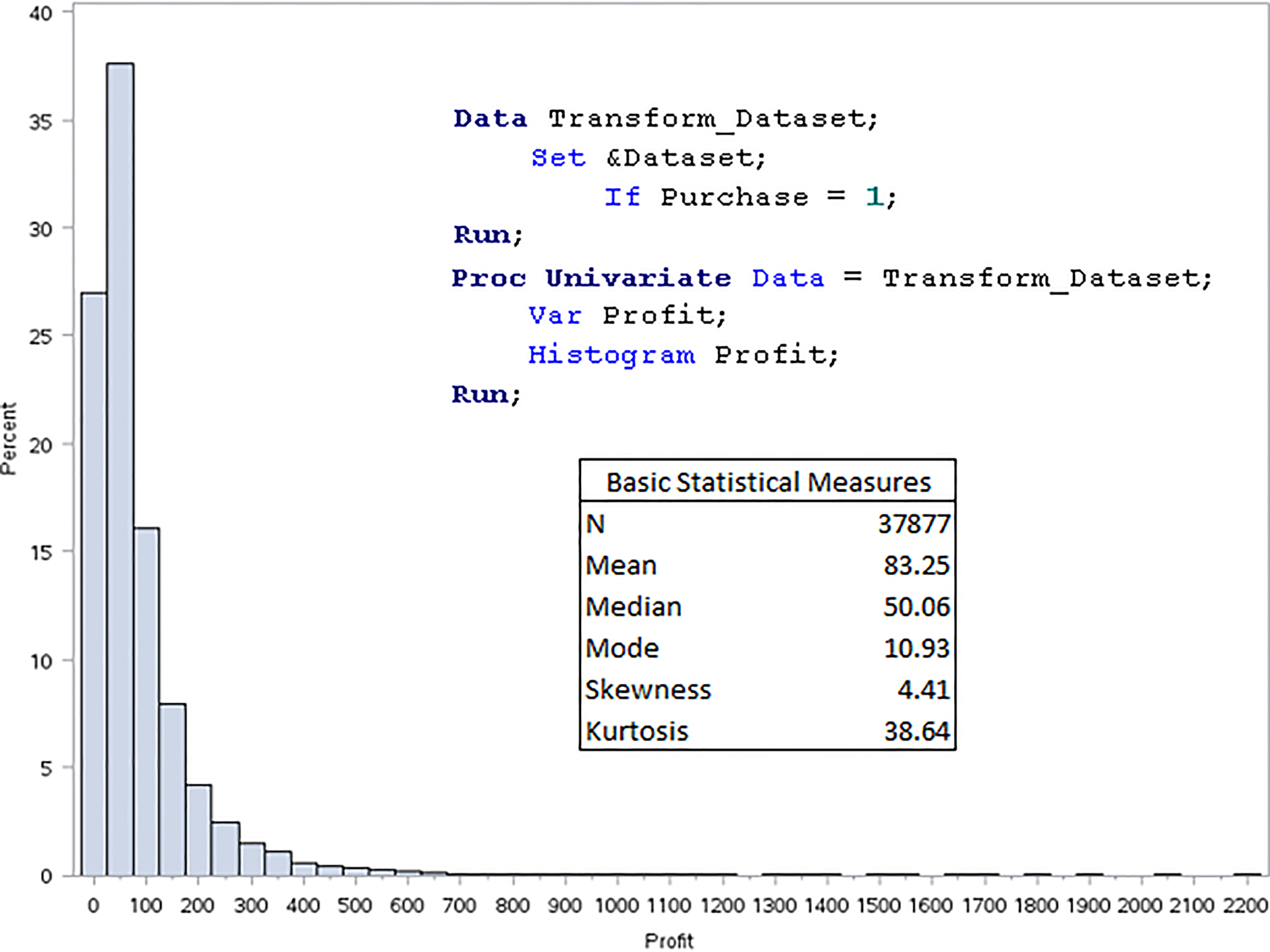

Figure 5.

Log transformed profit distribution (purchaser only).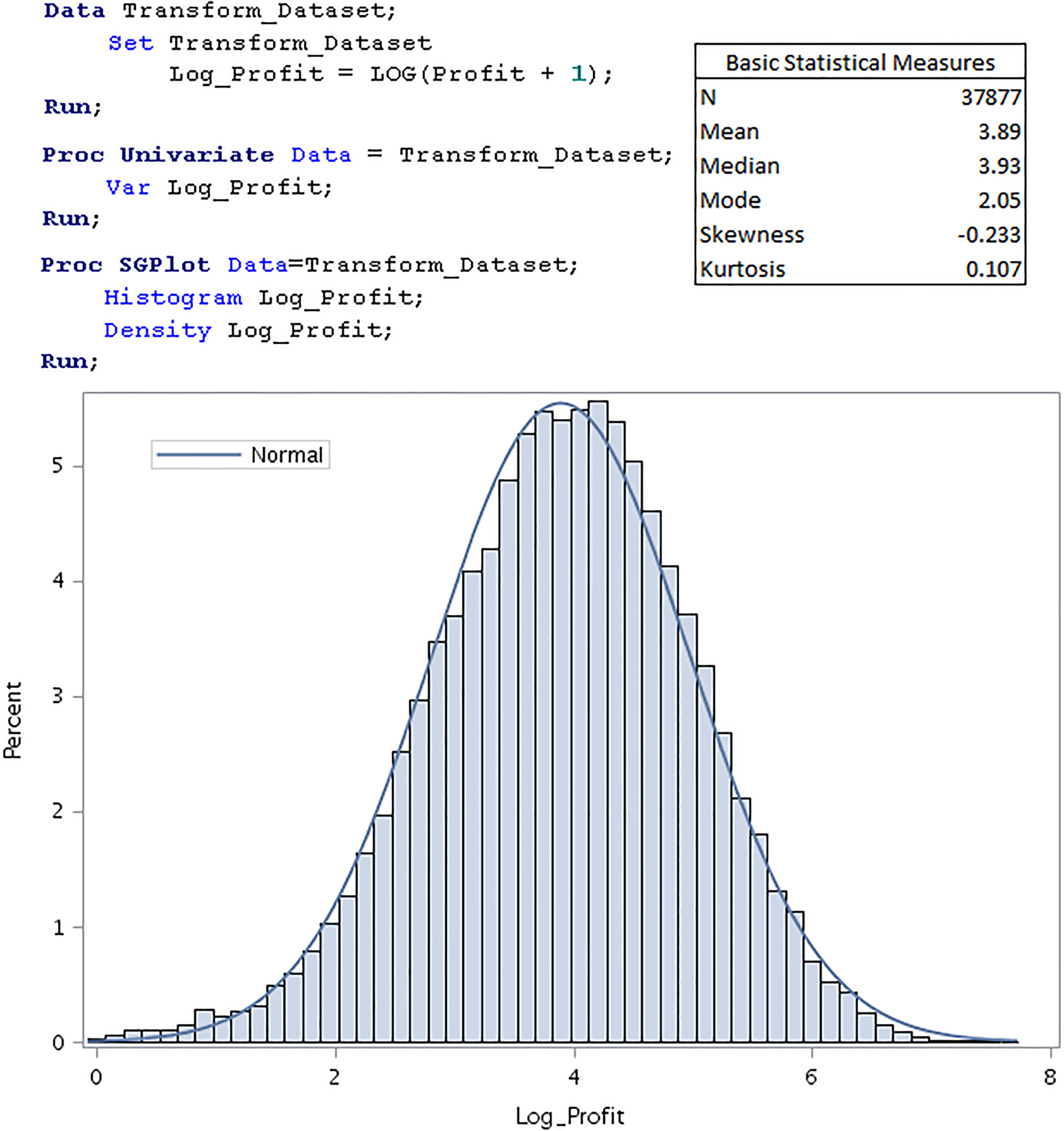

The data step and Proc Univariate routine in Fig. 4 serve to replicate the above but restrict the analysis to include only those customers who have made a purchase in the prediction period. The skewness and kurtosis figures have both come down but still not close to zero; the mean (83.3) and median (50.1) have even gone further apart. Again, such target distribution may still not be ideal for predictive modeling purposes.

To further mitigate the skewness problem, a logarithmic transformation: Log (Profit $+$ 1) is applied. The results as displayed in Fig. 5 show that both the skewness and kurtosis figures are now close to zero; and the mean (3.89) aligns with the median (3.93) closely. This log-transformed Profit target appears to follow a symmetric normal distribution, and this makes predictive modeling to be easier.

One may want to understand that the logarithmic transformation also helps to restrict the predicted conditional future profit to be non-negative (see Step 4.2). On the other hand, the normality of the log-transformed Profit makes the un-logging process in Step 4.2 to be simpler (see Eq. (5) in Section 3.2.3.3).

This exploratory analysis together with Sections 2.1 and 2.2 suggests the following steps to be undertaken towards the prediction of future profit.

Step 1.0:

Build Model 1 using the modeling dataset (Purchase: Not Purchase $=$ 1:1).

Step 2.0:

Build Model 2 using the Purchase group (i.e. records with Purchase $=$ 1) of the modeling dataset. The target: Profit to be log- transformed prior to modeling.

Step 3.1:

Use the confirmed Model 1 built to score (i.e. predict) the targeted audience of interest.

Step 3.2:

Adjust (i.e. undo under-sampling) the scored probability, and this adjusted probability is the likelihood of future purchase $P$ as shown in Fig. 1.

Step 4.1:

Use the confirmed Model 2 built to score the same targeted audience.

Step 4.2:

The scored profit, in log- transformed status, is then to be unlogged to obtain the desired conditional future profit, and this is the $ Profit as shown in Fig. 1.

Step 5.0:

Calculate the expected future profit which equals $P$ * $ Profit, and this is the predicted future profit of the audience.

3.2 Predictive modeling

This section uses SAS ${}^{\@setsize{\scriptsize}{8pt}{\viipt}{\@viipt}\textregistered}$ Enterprise Miner™ 13.2 to build predictive models. The upper portion of the diagram (Fig. 6) is the process for building Model 1 (Step 1.0) while the lower portion of the diagram is the process for building Model 2 (Step 2.0). Each of the two model winners is then used to score the test dataset: TEST_DATASET (Steps 3.1 and 4.1). The below portrays the predictive modeling analysis, and their corresponding results and interpretations.

Figure 6.

A process flow diagram for modeling the likelihood of future purchase and future profit.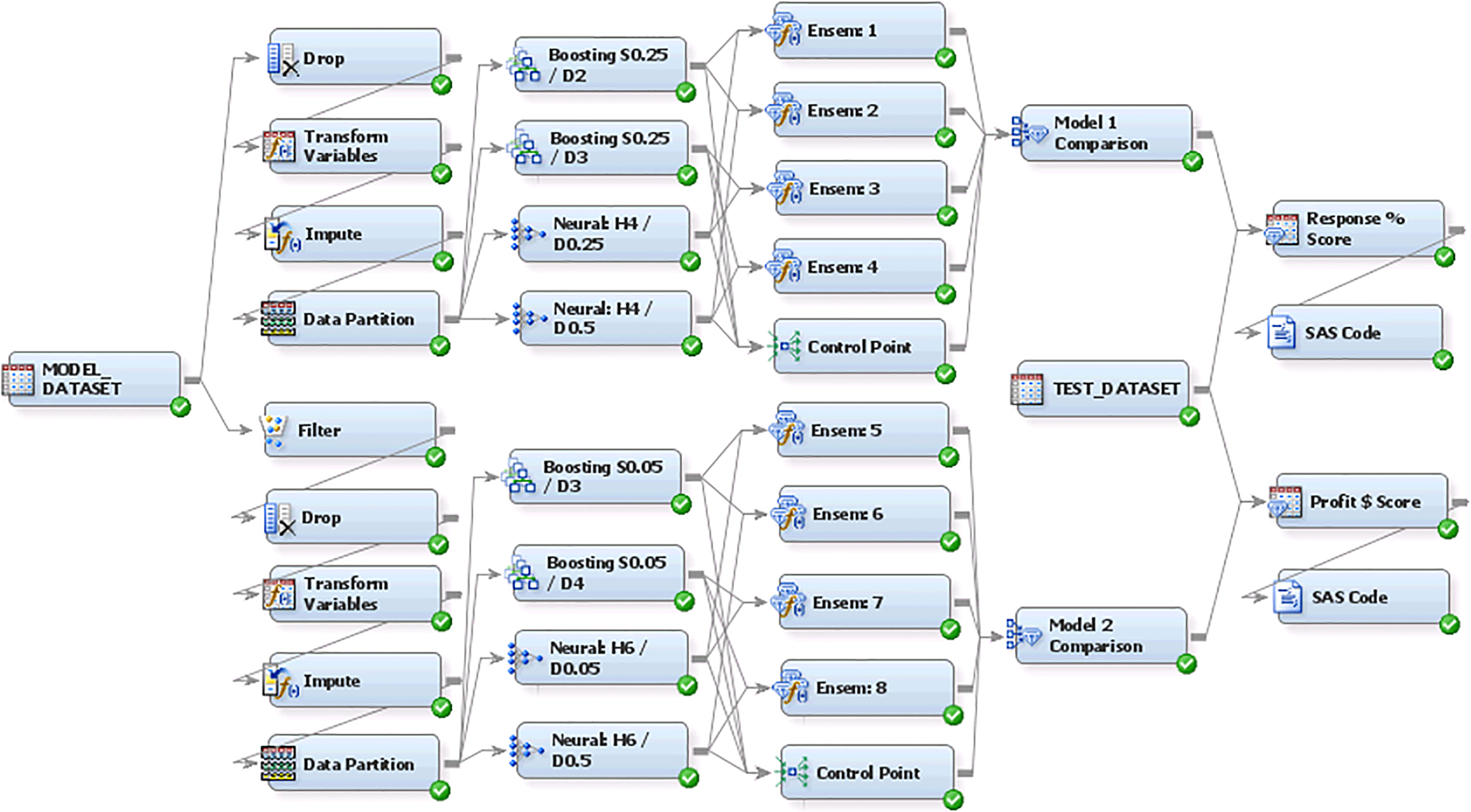

3.2.1 Highlights of some selective data processing and model nodes

Data

•
For the first data node: Model_Dataset, the role of the data source is set as Raw. The variable: Purchase is set as a binary target (Role $=$ Target and Level $=$ Binary) and the variable: Profit is set as an interval target (Role $=$ Target and Level $=$ Interval). For the second data node: TEST_DATASET, the role of the data source is set as Score and the Role of the variable: Purchase and Profit, are set as Reject.

Transform variables

•
In each of the two nodes, all interval input variables are set as “Best” for the method of transformation. This method tries all the available built-in alternatives (i.e. log, inverse, binning, etc.) and selects the one that the transformed input has the strongest R Squared relationship with the target. All binary input variables are set as “Default”, meaning no transformation. For the upper node, the binary target is set as “Default”; and the interval target in the lower node is set as “Log”.

Impute

•
In each of the two Impute nodes, all binary and interval input variables are set as “Tree” as the missing value imputation method.

Data partition

•
For each of the two nodes, the dataset is split into Training and Validation in the proportion of 50%–50%.

Gradient boosting

•
For all nodes, the assessment measure is set as “Average Squared Error”. Different combinations of the shrinkage constant (S) and maximum depth (D) have been experimented, and no vigorous attempt has been made for intensive hyper-parameter optimizations.

Neural network

•
For all nodes, the model selection criterion is set as “Average Squared Error”. Different combinations of the number of hidden units (H) and weight decay constant (D) have been tried, and again no attempt has been made for vigorous hyper-parameter optimizations.

Ensemble

•
The default “average” ensemble method is used for all ensemble nodes.

Model comparison

•
The model selection statistic is set as “Average Squared Error” for both Models 1 and 2.

3.2.2 Model comparison results

This sub-section displays the final model comparative results. In both the Models 1 and 2 scenarios, Neural Network performs better than Gradient Boosting; and all ensemble models (Ensem: 1 to Ensem: 8) outperform individual Neural Network and Gradient Boosting models.

In determining Model 1, Ensem: 3 (Boosting S0.25/D3 and Neural H4/D0.25) gives the lowest validation average squared error (Table 3) and is therefore selected as the model winner for the prediction of likelihood of future purchase. For Model 2, Ensem: 8 (Boosting S0.05/D4 and Neural H6/D0.5) records the lowest validation average squared error and therefore becomes the model winner for the prediction of conditional profit.

Table 3
Model performance comparison for determining Model 1 and 2

Model description	Validation average squared error
Model 1
Ensem: 3	0.115270
Ensem: 4	0.115295
Ensem: 1	0.115348
Ensem: 2	0.115367
Neural: H4/D0.25	0.115801
Neural: H4/D0.5	0.115856
Boosting: S0.25/D3	0.117737
Boosting: S0.25/D2	0.117801
Model 2
Ensem: 8	0.739440
Ensem: 6	0.739934
Ensem: 7	0.740407
Ensem: 5	0.740908
Neural: H6/D0.5	0.741453
Neural: H6/D0.05	0.741852
Boosting: S0.05/D4	0.778517
Boosting: S0.05/D3	0.779336

3.2.3 Overall model validation

Model 1 and Model 2 have been individually validated (e.g. via ROC chart, cumulative lift and mean predicted curve) with the validation datasets sampled in their corresponding Data Partition nodes (see Fig. 6). The details are not discussed in this paper. Alternatively, this section primarily attempts to use another holdout dataset (TEST_DATASET) to examine the joint validity of Model 1 and Model 2 in the prediction of future profit. This will involve scoring the TEST_DATASET (Step 3.1 and Step 4.1), adjusting the predicted probability (Step 3.2), re-engineering (un-logging) the conditional transformed future profit (Step 4.2), calculating the predicted future profit (Step 5.0), and building decile charts (to be illustrated).

3.2.3.1 Scoring

Each of the 73,075 observations in the TEST_DATASET is scored by Model 1 and Model 2 separately. Two data steps are written within their corresponding SAS Code nodes (Fig. 6), one for creating a data table (Scored_Purchase) to store the unadjusted purchase probability (i.e. “EM_EventProbability”) as predicted by Model 1, and the other one for creating another data table (Scored_Profit) to store the conditional transformed future profit (i.e. “EM_Prediction”) as predicted by Model 2.

3.2.3.2 Adjusting the scored probabilities

Since the majority group (Not Purchase) has been under sampled (see Table 1) to bring up the proportion of “Purchase” from 21.0% (a sample reflecting the entire population) to 50.0% (a biased sample) for modeling purposes, the scored probability needs to be adjusted. If the proportion of “Purchase” and “Not Purchase” in the representative sample are known to be $\pi_{1}$ and $\pi_{2}$ , and that if the proportion of “Purchase” and “Not Purchase” in the estimation sample equal $\rho_{1}$ and $\rho_{1}$ representatively, then the adjusted probability of “Purchase” (it goes similarly for “Not Purchase”) is given by the formula:

$\displaystyle P_{1}=\frac{\widehat{P_{1}}\left({\frac{\pi_{1}}{\rho_{1}}}% \right)}{\widehat{P_{1}}\left({\frac{\pi_{1}}{\rho_{1}}}\right)+\widehat{P_{0}% }\left({\frac{\pi_{0}}{\rho_{0}}}\right)}$ (4)

where $\widehat{P_{1}}$ and $\widehat{P_{0}}$ represent the unadjusted predicted probability of Purchase and Not Purchase respectively, and $\widehat{P_{1}}+\widehat{P_{0}}=$ 1. Interested parties may refer to Sarma (2013, p. 235) for further details. Given that:

$\rho_{1}=$ 0.5 (i.e. $\rho_{2}=$ 0.5), $\pi_{1}=$ 0.2104278 (i.e. $\pi_{2}=$ 0.7897722), $\widehat{P_{1}}=$ EM_EventProbability, (i.e. $\widehat{P_{2}}=1$ – EM_EventProbability),

the adjusted probability of “Purchase”: $P_{1}$ followed. A new dataset (ReScaled_Purchase) was created to store $P_{1}$ in addition to the EM_EventProbability.

3.2.3.3 Un-logging the scored profits and predicting future profit

A new dataset (Model_Purchase_Profit) was compiled. The process merged the two scored datasets (ReScaled_ Purchase and Scored_Profit). It also calculated and stored the predicted future profit: “Predicted Future Profit”. Given $Y=\log\left({Y^{\ast}+1}\right)$ to be normally distributed with mean $\mu$ and variance $\sigma^{2}$ , it can be deduced that the expected value of $Y^{\ast}$ is given by:

$\displaystyle E(Y^{\ast})=\textit{EXP}\left({\mu+\sigma^{2}/2}\right)-1$ (5)

Those who are interested in Eq. (5) may refer to Malthouse (2013, p. 136) for more detailed explanation. In our scenario, the scored profit is an estimate of the mean, and the square of the standard error of the estimate $\textit{SE}^{2}$ can be taken as an estimate of the variance. The estimation formula for the “Predicted Future Profit”, with the un-logging and adjustment of the non-purchaser bias, can be written as

$\displaystyle\text{Predicted Future Profit}=\left({\textit{EXP}\left({\textit{% SP}+\textit{SE}^{2}/2}\right)-1}\right)$ (6)

where SP is the scored profit (i.e. “EM_Prediction”), and the validation average squared error (or mean squared error “MSE”): 0.73944 from the Model 2 winner (Ensem: 8) has been taken as the $\textit{SE}^{2}$ .

3.2.3.4 Construction of semi-decile charts

The table: Model_Purchase_Profit is then merged with the original TEST_DATASET to form a table: Model_Vs_Actual. This new table now stores the predicted probability of purchase: “ReScaled_Prob” and the “Predicted Future Profit”, as well as their corresponding sampled actuals (“Purchase” and “Profit”). One would naturally want to compare these predicted values versus actuals for the purposes of validation. This can be achieved by using some form of decile table. Since the sample size is large enough, semi-decile (i.e. 20 ranks) is used instead. The validation results are displayed in Tables 4 and 5.

Table 4

Semi-decile table for the probability of purchase

Semi-decile	Count	Model (%)	Actual (%)
1	3,653	87.9	86.8
2	3,654	73.3	69.5
3	3,654	62.5	65.0
4	3,653	52.0	54.2
5	3,654	41.4	42.1
6	3,654	31.2	31.4
7	3,654	21.8	22.3
8	3,653	15.5	15.2
9	3,654	11.5	11.6
10	3,654	8.6	8.7
11	3,654	6.0	5.4
12	3,653	3.7	3.7
13	3,654	2.3	2.3
14	3,654	1.5	1.3
15	3,654	0.9	0.7
16	3,653	0.6	0.4
17	3,654	0.4	0.1
18	3,654	0.2	0.1
19	3,654	0.1	0.0
20	3,654	0.1	0.0
Total	73,075	21.1	21.0

Table 5

Semi-decile table for the (unconditional) predicted future profit

Semi-decile	Count	Model ($)	Actual ($)	MAE ($)
1	3,653	160.8	147.3	109.1
2	3,654	68.1	64.1	58.5
3	3,654	44.4	39.9	43.0
4	3,653	31.1	28.7	33.7
5	3,654	22.2	20.2	26.4
6	3,654	15.7	15.4	21.1
7	3,654	11.0	11.2	16.7
8	3,653	7.6	6.9	11.7
9	3,654	5.3	5.2	9.0
10	3,654	3.7	3.4	6.3
11	3,654	2.4	2.5	4.6
12	3,653	1.5	1.6	3.0
13	3,654	0.9	0.9	1.7
14	3,654	0.5	0.6	1.1
15	3,654	0.3	0.2	0.5
16	3,653	0.2	0.1	0.3
17	3,654	0.1	0.0	0.1
18	3,654	0.1	0.0	0.1
19	3,654	0.0	0.0	0.0
20	3,654	0.0	0.0	0.0
Total	73,075	18.8	17.4	17.4

In each semi-decile in Table 4, the average Model probability and the Actual proportion of purchase is very close (i.e. accurate). The Actuals give a monotonic decreasing pattern down the semi-decile. There is also a high differentiation in Actuals between the top and bottom semi-decile. All these are good signs, suggesting that Model 1 is of high validity for the prediction of probability of purchase.

Table 5 shows that the average Model profit (i.e. “Predicted Future Profit”) is also quite close to the average Actual profit in each semi-decile, albeit the fact that the accuracy does not visually appear to be as good as the case for the prediction of probability of purchase. The monotonic decreasing pattern down the semi-decile as well as the high differentiation in Actuals between the top and bottom semi-decile both also look very positive. Again, all these suggest that the combined effort of Models 1 and 2 has resulted in good validity for the prediction of future profit.

Each measure MAE (mean absolute error) is quite sizable and comparable to its corresponding Model and Actual values. The high variance reflects the fact that there is a high proportion (79.0%) of zero-value Actual observations whereas each Model value is always above zero. This may suggest that while the future profit can be individually predicted, it is better to be aggregately presented and interpreted in the segment level.

4. Conclusion

This paper has illustrated a methodological framework for predicting the future profit for customer purchases of non-contractual products. The skewness of the profit distribution has been demonstrated and a two-stage model was proposed. Stage 1 has produced an ensemble model: Model 1, which is consisted of a Gradient Boosting (with Shrinkage $=$ 0.25 and Depth $=$ 3) and a Neural Network (with 4 Hidden Nodes and Decay $=$ 0.25) model. This ensemble Model 1 has achieved a validation average squared error of 0.11527, which is slightly better than any of its two constituents (validation ASE $=$ 0.11774 and 0.11580 for Gradient Boosting and Neural Network respectively). Similarly, Stage 2 has produced an ensemble model: Model 2, which is consisted of a Gradient Boosting (with Shrinkage $=$ 0.05 and Depth $=$ 4) and a Neural Network (with 6 Hidden Nodes and Decay $=$ 0.5) model. This ensemble Model 2 has recorded a validation average squared error of 0.73944, which is again slightly better than any of its two constituents (validation ASE $=$ 0.77852 and 0.74145 for Gradient Boosting and Neural Network respectively). Each of the two model winners has been applied to a hold-out dataset. Two semi-decile tables have been constructed and they confirmed that Model 1 and Model 2 gave good validation predictions for both the likelihood of purchase as well as the (unconditional) future profit.

5. Managerial and research implications

While the presented methodological framework in this paper is extendable to cover a longer lifetime horizon, management may find this first-period focused version to be applicable in their business planning.

•

It is not uncommon for any business to focus on a shorter time frame, especially during the annual budgeting period. The proposed one-year focus can help the business to estimate the aggregated one-year average predicted future profit for any customer segment of interest.

•

It is not easy to evaluate the external validity of a lifetime value or longer-term prediction model in real life. In general, management is not in a position to wait for a few years (e.g. 5 years) to confirm the model accuracy, and some businesses may not even have a few years of customer history for a longer-term prediction. A one-year period is more affordable and feasible.

•

Marketing may want to evaluate and compare the values of customers acquired from different channel sources (e.g. search engine, social media and affinity program) in order to better allocate marketing budgets. A business intelligence report showing the aggregated average one-year predicted future profit by acquisition sources would give appropriate direction.

Researchers and analysts may continue to extend the current methodology to suit their business applications.

•

A two-stage model was found to be appropriate in the current analysis. In fact, some businesses may involve an analysis universe that is better represented by more than two component populations (e.g. non-buyer vs seasonal buyer vs non-seasonal buyer), and this may call for fitting a more complex model.

•

The author of this paper has prior understanding that neural network and gradient boosting work well with the customer base of the used business setting. In practice, researchers may need to experiment other data-mining techniques to work out a good ensemble model to suit their businesses.

•

The final profit assessment of the ensemble model in this study is primarily based on the semi-decile table (an aggregate measurement method), and it was found that the MAE (an individual-level measurement method) is quite high (due to the excess zero profit). Researchers may continue exploring better ways to improve the prediction accuracy in the individual customer level.

Footnotes

Acknowledgments

The author is grateful to Professor Manoj Agarwal, Binghamton University, SUNY, for the review of this paper.

Operational definitions

•

Future profit – The profit that a customer (without prior knowledge as to whether he will make a purchase) would generate during a time-period in the future, and is the primary item for prediction in this analysis.

•

Conditional future profit – The profit that a customer would generate during a time-period in the future given the customer would make a purchase.

•

Expected future profit – This is a statistical quantity after the adjustment of non-purchaser bias, and this quantity is used as the prediction of the future profit in this study.

•

Likelihood of future purchase – This refers to the probability of purchase in the future time-period.

•

Customer lifetime value – This is a marketing term which refers to the total profit a customer generates during his entire lifetime. It is often loosely taken as the prediction of residual lifetime value counting from a particular point in time onwards, or defined as the profit generated during a longer period of time in the future. It is to be used interchangeably with customer value in this paper.

•

Neural network – A predictive data-mining technique that emulates a biological neural network of the human brain. It is based on a collection of connected nodes (like neurons). The network is trained to perform a particular function by adjusting the values (weights) between connected nodes.

•

Gradient boosting – A predictive data-mining technique based on a series of models developed in the sequential (vertical) manner. When confined to tree based models, the tree created in the sequence uses the residuals from the tree created in the previous step as the target.

•

Ensemble – A method in combining different data-mining techniques to attempt to reach better predictive accuracy.

References

Damn,

, & Monroy,

C.R.

(2011). A review of the customer lifetime value as a customer profitability measure in the context of customer relationship management. Intangible Capital, 7(2), 261-279.

Dunford,

Su,

Tamang,

, & Wintour,

(2014). The Pareto Principle. The Plymouth Student Scientist, 7(1), 140-148.

Erdman,

Jackson,

, & Sinko,

(2008). Zero-Inflated Poisson and Zero-Inflated Negative Binomial Models Using the COUNTREG Procedure. Proceedings of the SAS Global Forum 2008, Cary, NC: SAS Institute Inc.

EsmaeiliGookeh,

, & Tarokh,

M.J.

(2013 December). Customer Lifetime Value Models: A Literature Survey. International Journal of Industrial Engineering & Production Research, 24(4), 317-336.

Farder,

P.S.

, & Hardie,

B.G.S.

(2009 February). Probability Models for Customer-Base Analysis. Journal of Interactive Marketing, 23(1), 61-69.

Huang,

, & Xie,

(2012). Modeling Loss Given Default (LGD) by Finite Mixture Model. The Northeast SAS User Group 2012 Conference.

Kapitula,

L.R.

(2015). When Two Are Better Than One: Fitting Two-Part Models Using SAS

{}^{\@setsize{\tiny}{6pt}{\vpt}{\@vpt}\textregistered}

. Proceedings of the SAS Global Forum 2015, Cary, NC: SAS Institute Inc.

Kessler,

, & McDowell,

(2012). Introducing the FMM Procedure for Finite Mixture Models. Proceedings of the SAS Global Forum 2012, Cary, NC: SAS Institute Inc.

Kotler,

(1974). Marketing During Periods of Shortage. Journal of Marketing, 38(3), 20-29.

10.

Liu,

Nguyen,

T.T.

Zhao,

Zha,

Yang,

Cao,

Wu,

Zhao,

, & Chen,

(2016). Repeat Buyer Prediction for Ecommerce. Proceedings of the 22nd ACM SIGKDD International Conference on Knowledge Discovery and Data Mining, ACM, pp. 155-164.

11.

Lu,

(2003). Modeling Customer Lifetime Value Using Survival Analysis – An Application in the Telecommunications Industry. Proceedings of the 28

{}^{\text{th}}

Annual SAS Users Group International Conference SUGI 28, 2003.

12.

Lund,

(2015). Multinomial Logistic Model for Long-Term Value. Proceedings of the SAS Global Forum 2015, Cary, NC: SAS Institute Inc.

13.

Lund,

(2016). Probability Density for Repeated Events. Proceedings of the SAS Global Forum 2016, Cary, NC: SAS Institute Inc.

14.

Malthouse,

E.C.

(2013). Segmentation and Lifetime Value Models Using SAS

{}^{\@setsize{\tiny}{6pt}{\vpt}{\@vpt}\textregistered}

. Cary, NC: SAS Institute Inc.

15.

Malthouse,

E.C.

, & Blattberg,

R.C.

(2005 Winter). Can We Predict Customer Lifetime Value? Journal of Interactive Marketing, 1(19), 2-16.

16.

Mulhern,

F.J.

(1999 Winter). Customer Profitability Analysis: Measurement, Concentration, and Research Directions. Journal of Interactive Marketing, 13(1), 25-40.

17.

Pfeifer,

P.E.

, & Carraway,

R.L.

(2000 Spring). Modeling Customer Relationship as Markov Chains. Journal of Interactive Marketing, 14(2), 43-55.

18.

Pliner,

(2016). Customer Lifetime Value Modeling. Proceedings of the SAS Global Forum 2016, Cary, NC: SAS Institute Inc.

19.

Sarma,

K.S.

(2013). Predictive Modeling with SAS

{}^{\@setsize{\tiny}{6pt}{\vpt}{\@vpt}\textregistered}

Enterprise Miner™: Practical Solution for Business Applications, Second Edition. Cary, NC: SAS Institute Inc.

20.

Singh,

, & Jain,

(2010). Measuring Customer Lifetime Value: Models and Analysis. Review of Marketing Research.

21.

Thatte,

, & Chakraborty,

(2015). A mathematical model for optimizing product mix and customer lifetime value. Proceedings of the SAS Global Forum 2015, Cary, NC: SAS Institute Inc.