The Marshall-Olkin extended flexible Weibull regression model for censored lifetime data

Abstract

We study some mathematical properties of a new generator of continuous distributions with one additional shape parameter named the Marshall-Olkin extended-G (MOE-G) family. We propose a new distribution called the MOE-Flexible Weibull and obtain some of its structural properties. Further, we construct a regression model based on this distribution with two systematic components that can be applied to real lifetime data. We estimate its model parameters by maximum likelihood. We present a diagnostic analysis based on global influence and deviance residuals. Two real data sets are used to illustrate the potentiality of the proposed models.

Keywords

Censored data flexible weibull distribution Marshall-Olkin family maximum likelihood estimation regression model

1. Introduction

In survival analysis applications, the failure rate may have frequently unimodal or bathtub shape, that is, non-monotone functions. The regression models commonly used for survival studies are the log-Weibull (monotone failure rate shape) and log-logistic (decreasing or unimodal failure rate shape). In the first part of the paper, we define the new Marshall-Olkin extended-G (MOE-G) family and propose the MOE-Flexible Weibull (MOE-FW) distribution. The advantage of this distribution is its flexibility in accommodating several forms of the hazard rate function (hrf), for instance, increasing-decreasing-increasing, bathtub and unimodal shapes. It is also suitable for testing the goodness-of-fit in relation to nested models, for example, with the flexible Weibull distribution by using the likelihood ratio test.

Also, Marshall and Olkin (1997) proposed an interesting method for obtaining more flexible distributions by adding a new parameter to a baseline distribution yielding the called Marshall-Olkin (MO) family of distributions. This family includes the parent distribution as a basic exemplar and gives more flexibility to some distributions for modeling various types of data. The MO family is also known as the proportional odds family (proportional odds model) or family with tilt parameter (Marshall & Olkin, 2007). Recently, the MO family has been used in several research areas such as engineering, hydrology and survival analysis. For example, Barreto-Souza et al. (2013) presented some general results for this family, Cordeiro et al. (2014) investigated more mathematical properties for it and defined new models, Krishna et al. (2013) analyzed some applications of Marshal-Olkin Fréchet distribution and Alizadeh et al. (2015) introduced the Kumaraswamy Marshal-Olkin family.

In the second part, we introduce a regression model with two systematic structures based on the MOE-FW distribution for modeling censored data with bathtub-shaped hrf. We consider a classical analysis for the parameters of this regression model and present some ways to perform global influence and residual analysis based on deviance residuals. For different parameter settings, sample sizes and under the mechanism of random censoring on the right and censoring percentages, we perform various simulation studies and the empirical distribution of the deviance residuals is displayed and compared with the standard normal distribution. These studies reveal that the empirical distribution of the deviance residuals for the MOE-FW regression model with censored data has a good agreement with the standard normal distribution.

The article is organized as follows. In Section 2, we define the MOE-G family and the MOE-FW distribution. In Section 3, we derive two useful expansions and obtain some mathematical properties for the MOE-FW distribution including ordinary and incomplete moments and generating functions. Maximum likelihood estimation of the model parameters is addressed in Section 4. We also perform various simulations to investigate the behavior of the maximum likelihood estimators (MLEs) for different parameter settings, sample sizes and under the mechanism of random censoring on the right, censoring percentages. Based on the MOE-FW distribution, we define in Section 5 a regression model with two systematic structures for censored lifetime data. Diagnostics and residual analysis are discussed in Section 6. In Section 7, we provide two applications to real data. Section 8 ends with some concluding remarks.

2. Marshall-Olkin extended family

Hundreds of articles on continuous univariate lifetime distributions have been published in recent years. Adding parameters to a well-established distribution is a is a time-honored device for obtaining more flexible classes of distributions. Recent developments have been made to define new generated families to control skewness and kurtosis through the tail weights and provide great flexibility in modeling skewed data in practice.

Let $G(t)=G(t;\bm{\tau})$ be a baseline cumulative distribution function (cdf) and $\bar{G}(t;\bm{\tau})=1-G(t;\bm{\tau})$ be the corresponding survival function of a continuous random variable $W$ , where $\bm{\tau}=(\tau_{1},\cdots,\tau_{q})^{\top}$ is a parameter vector of dimension $q$ . Further, let $g(t)=g(t;\bm{\tau})$ be the probability density function (pdf) of $W$ . The MO family cdf, say ${F}(t)={F}(t;a,\bm{\tau})$ , is defined by

$\displaystyle{F}(t)=1-\frac{a\bar{G}(t;\bm{\tau})}{1-\bar{a}\bar{G}(t;\bm{\tau% })}=1-\frac{a\bar{G}(t;\bm{\tau})}{G(t;\bm{\tau})+a\bar{G}(t;\bm{\tau})},\quad t% \in\mathbb{R},\quad a>0,$ (1)

where $\bar{a}=1-a$ . Clearly, Eq. (1) provides a flexible tool to obtain new parametric distributions from existing ones. For $a=$ 1, $\bar{F}(t)=\bar{G}(t;\bm{\tau})$ and therefore $\bar{G}(x;\bm{\tau})$ is a basic exemplar of Eq. (1). The MO family density, say ${f}(t)={f}(t;a,\bm{\tau})$ , is given by

$\displaystyle f(t)=\frac{a\,g(t;\bm{\tau})}{[1-\bar{a}\bar{G}(t;\bm{\tau})]^{2% }},\quad t\in\mathbb{R}.$ (2)

We define the MOE-G family from Eq. (1) with an additional shape parameter $b>$ 0 by changing $\bar{G}(t;\bm{\tau})$ by $[1-G(t;\bm{\tau})]^{b}$ . Hence, the general form for the MOE-G family cdf is

$\displaystyle F(t)=F(t;a,b,\bm{\tau})=1-\frac{a[1-G(t;\bm{\tau})]^{b}}{1-(1-a)% [1-G(t;\bm{\tau})]^{b}},$ (3)

where $a>$ 0 and $b>$ 0 are two additional shape parameters. For $b=$ 1, we obtain the MO family. The baseline distribution follows from Eq. (3) when $a=b=$ 1. A good point for the new family is that Eq. (3) does not involve any complicated function.

The MOE-G density reduces to

$\displaystyle f(t)=f(t;a,b,\bm{\tau})=a\,b\,g(t;\bm{\tau})[1-G(t;\bm{\tau})]^{% b-1}\,\left\{1-(1-a)[1-G(t;\bm{\tau})]^{b}\right\}^{-2}.$ (4)

The density Eq. (4) allows for greater flexibility of its tails and can be widely applied in many areas. We can define from Eq. (4) several new models for survival and reliability analysis.

In this research, we focus on extending the FW distribution introduced by Bebbington et al. (2007), since it is a very flexible distribution and little explored in survival analysis. The cdf and pdf of the FW distribution with two shape parameters $\alpha>$ 0 and $\beta>$ 0 are given by

$\displaystyle G(t;\alpha,\beta)=1-\exp\left[-\exp\left(\alpha\,t-\frac{\beta}{% t}\right)\right],\quad t>0,$ (5)

and

$\displaystyle g(t;\alpha,\beta)=\left(\alpha+\frac{\beta}{t^{2}}\right)\exp% \left[\left(\alpha\,t-\frac{\beta}{t}\right)-\exp\left(\alpha\,t-\frac{\beta}{% t}\right)\right],$ (6)

respectively. For $\beta=$ 0 and $\alpha=\log(\lambda)$ , $\lambda>$ 0, we have the exponential cdf $G(t)=1-\exp(-\lambda\,t)$ .

We are motivated to introduce the MOE-FW distribution because of the above generalizations, the wide usage of the Weibull distribution and the fact that the current generalization provides means of its continuous extension to still more complex situations. We study some of its mathematical properties.

The MOE-FW density is defined from Eq. (4) by taking $G(t;\bm{\tau})$ and $g(t;\bm{\tau})$ as the cdf and pdf of the FW $(\alpha,\beta)$ distribution, namely (for $t>$ 0)

$\displaystyle f_{\textit{MOE-FW}}=a\,b\,\left(\alpha+{\beta}/{t^{2}}\right)% \exp\left[\alpha\,t+{\beta}/{t}-\kappa_{\alpha\beta}(t)\right]\exp[-(b-1)% \kappa_{\alpha\beta}(t)]\times\left\{1-(1-a)\exp\left[-b\,\kappa_{\alpha\beta}% (t)\right]\right\}^{-2},$ (7)

where $\kappa_{\alpha\beta}(t)=\exp(\alpha\,t-\beta/t)$ , and $\alpha>$ 0 and $\beta>$ 0 are shape parameters.

Henceforth, a random variable with pdf Eq. (7) is denoted by $T\sim$ MOE-FW $(a,b,\alpha,\beta)$ . For $b=$ 1, we obtain the MO-FW distribution. The FW distribution follows when $a=b=$ 1.

The MOE-FW survival function is given by

$\displaystyle S_{\textit{MOE-FW}}=\frac{a\exp[-b\,\kappa_{\alpha\beta}(t)]}{1-% (1-a)\exp[-b\,\kappa_{\alpha\beta}(t)]}.$ (8)

The hrf of the MOE-FW distribution reduces to

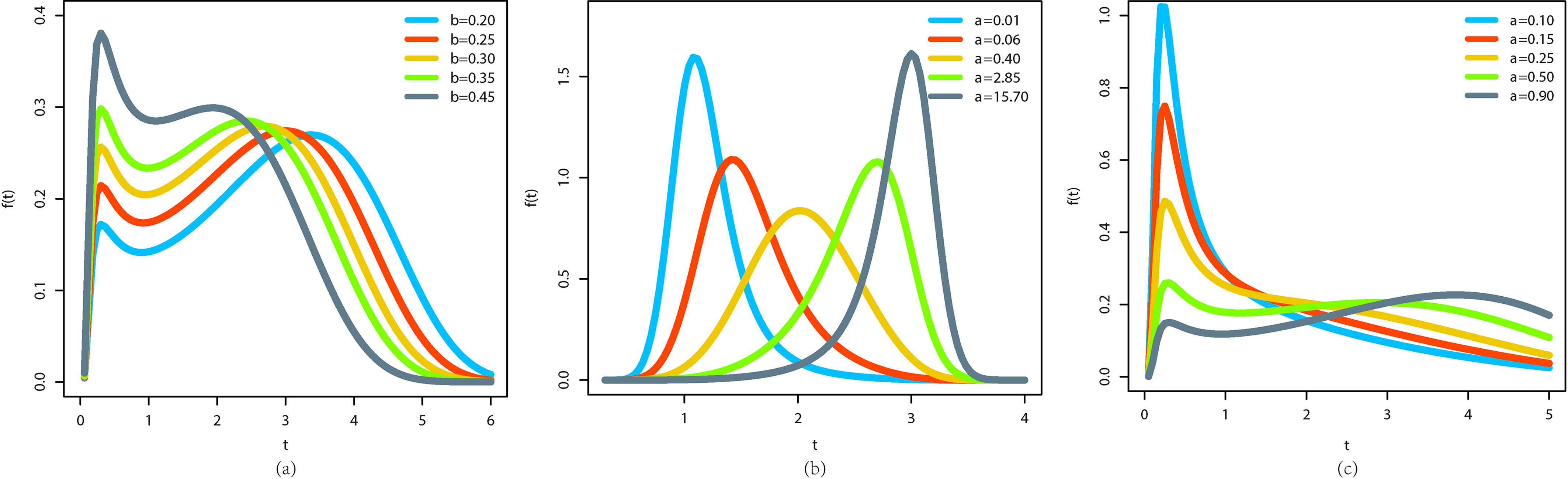
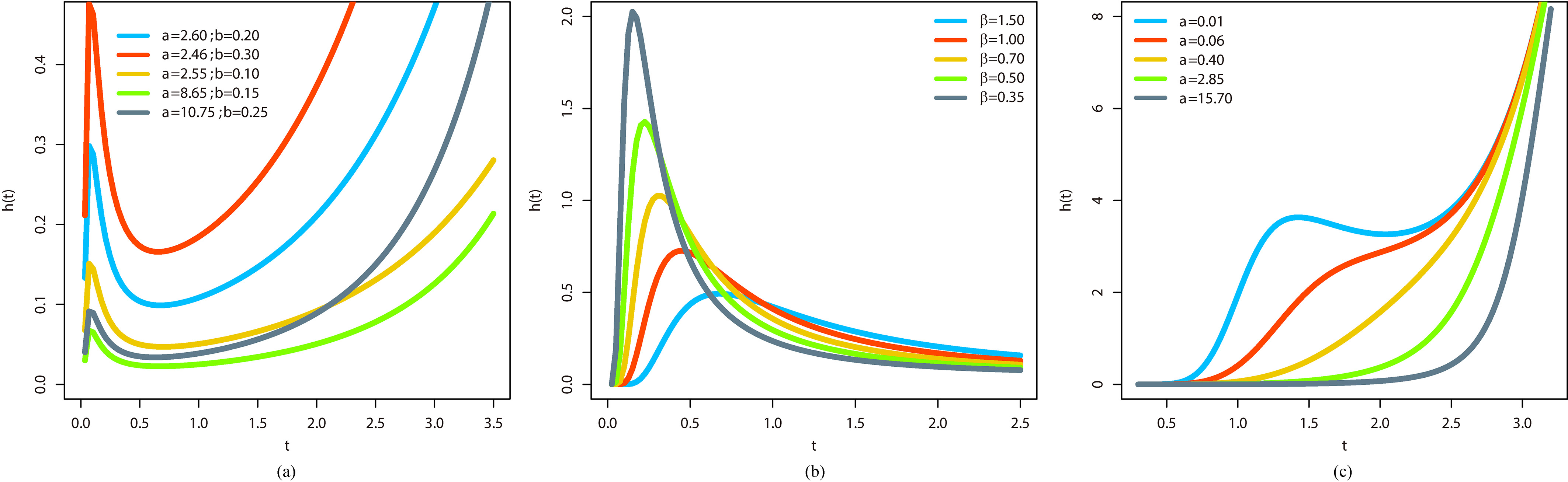
$\displaystyle h_{\textit{MOE-FW}}=\frac{b\,(\alpha+\beta/t^{2})\exp(\alpha\,t+% \beta/t)}{1-(1-a)\exp[-b\,\kappa_{\alpha\beta}(t)]}.$ (9)

Some possible shapes of the density Eq. (7) and hazard function Eq. (9) for selected parameter values, including well-known distributions, are displayed in Figs 1 and 2, respectively. An important characteristic of the new distribution is that the MOE-FW density has bimodal shapes. Further, its hrf can be bathtub shaped, monotonically increasing or decreasing, monotonically increasing, decreasing and increasing and upside-down bathtub depending basically on the parameter values.

Figure 1.

Plots of the MOE-FW density for some parameter values. (a) Fixed $\alpha=$ 0.60, $\beta=$ 0.50 and $a=$ 1.60. (b) Fixed $\alpha=$ 1.30, $\beta=$ 6.40 and $b=$ 0.55. (c) Fixed $\alpha=$ 0.60, $\beta=$ 0.50 and $b=$ 0.10.

Figure 2.

Plots of the MOE-FW hrf for some parameter values. (a) Fixed $\alpha=$ 0.60 and $\beta=$ 0.15. (b) Fixed $\alpha=$ 1.30, $\beta=$ 6.40 and $b=$ 0.55. (c) Fixed $\alpha=$ 0.06, $a=$ 0.10 and $b=$ 0.15.

3. Useful expansions

.

Let $T$ be a random variable having the MOE-G family. The cdf of $T$ can be expressed as

$\displaystyle F(t)=\sum_{k=0}^{\infty}w_{k}\,H_{k}(t),$ (10)

where

$\displaystyle w_{k}=w_{k}(a,b)=d_{0}^{-1}\,\left(e_{k}-\sum_{m=1}^{k}d_{k}\,e_% {k-m}\right),$

and $H_{k}(t)=G(t)^{k}$ is the exponentiated-G (exp-G) cdf with power parameter $k$ .

Proof: We consider the power series expansion

$\displaystyle(1-u)^{p}=\sum_{k=0}^{\infty}(-1)^{k}\,{p\choose k}\binom{p}{k}\,% u^{k},$ (11)

valid for any real non-integer $p$ and $|u|<$ 1.

After some algebra, we can rewrite Eq. (3) using Eq. (11) as

$\displaystyle F(t)=1-\frac{\sum_{k=0}^{\infty}e_{k}\,G(t)^{k}}{\sum_{k=0}^{% \infty}d_{k}\,G(t)^{k}},$

where $e_{k}=e_{k}(a,b)=(-1)^{k}\,a\,\binom{b}{k}$ , $d_{k}=d_{k}(a,b)=1-c_{k}$ $(\forall\,k\geqslant 0)$ and $c_{k}=c_{k}(a,b)=(-1)^{k}\,(1-a)\,\binom{b}{k}$ .

By using the result for the ratio of two power series in the last equation, we obtain Eq. (10).

.

The corresponding pdf of $T$ is given by

$\displaystyle f(t)=\sum_{k=0}^{\infty}w_{k+1}\,h_{k+1}(t),$ (12)

where $h_{k+1}(t)=(k+1)\,G(t)^{k}\,g(t)$ is the exp-G density with power parameter $k+1$ .

Theorems 1 and 2 are the main results of this section. Equation (12) reveals that the MOE-G density function is a linear combination of exp-G densities. So, some of its structural properties such as moments and generating function can be determined from those properties of the exp-G distribution.

3.1 Quantile function

Equation (3) has tractable properties especially for simulation, since its quantile function (qf) has the simple form

$\displaystyle t_{u}=Q_{G}\left(1-\left[\frac{1-U}{1+(a-1)U}\right]^{1/b}\right),$

where $U\sim$ Uniform $(0,1)$ and $Q_{G}(u)=G^{-1}(u)$ is the baseline qf.

Thus, the qf of the MOE-FW distribution is

$\displaystyle Q_{\textit{MOE-FW}}(u)=Q_{\textit{FW}}\left(1-\left[\frac{1-U}{1% +(a-1)U}\right]^{1/b}\right),$ (13)

where $G_{\textit{FW}}(\cdot)$ is the FW qf.

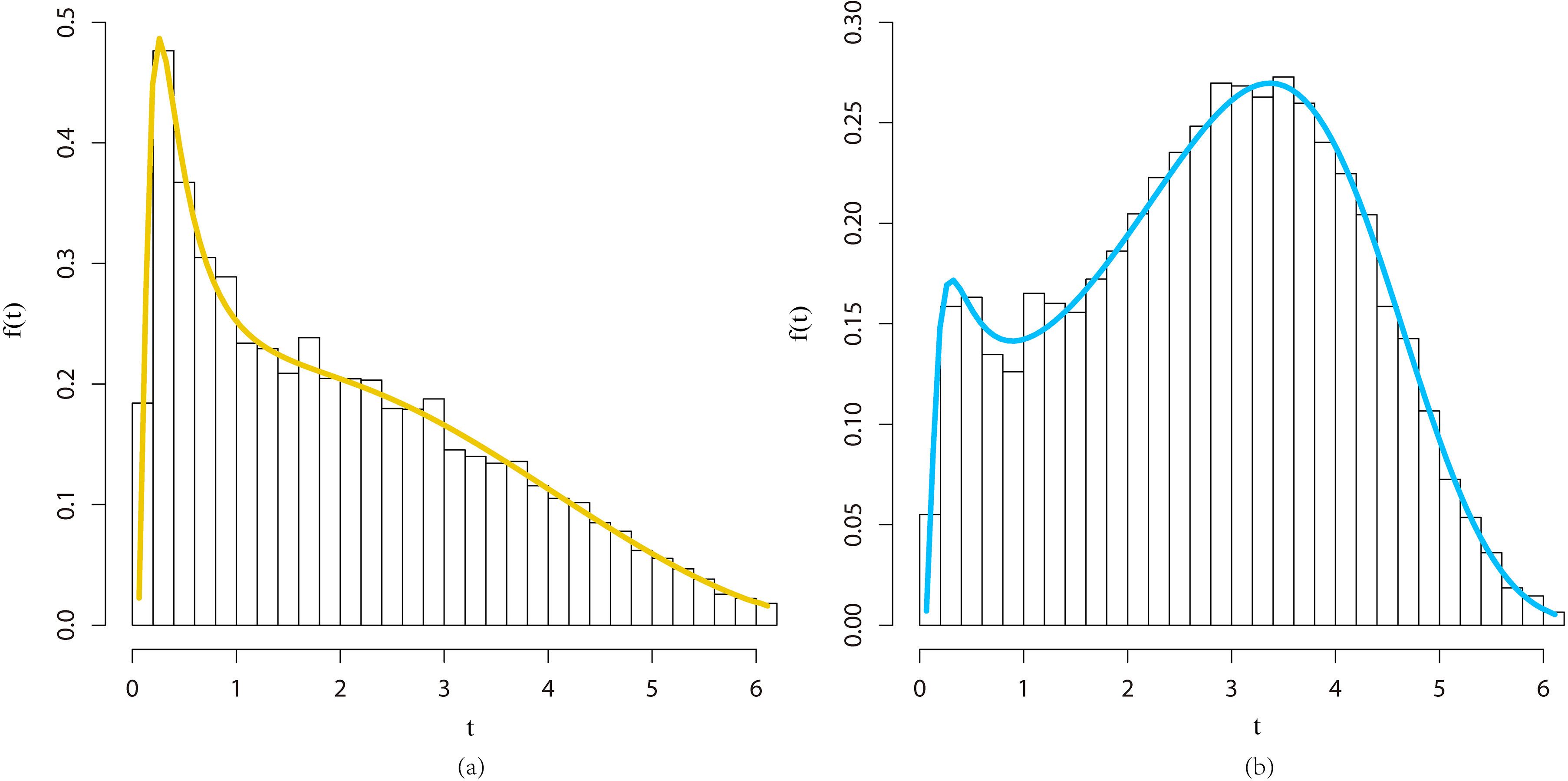
We provide plots of the MOE-FW density and histograms in Fig. 3 based on 10,000 replications for two parameter scenarios by using the $Q(u)=Q_{\textit{MOE-FW}}(u)$ function.

Figure 3.

Histograms and plots of the MOE-FW density. (a) $\alpha=$ 0.60, $\beta=$ 0.50, $a=$ 0.25 and $b=$ 0.10. (b) $\alpha=$ 0.60, $\beta=$ 0.50, $a=$ 1.60 and $b=$ 0.20.

Further, we calculate two important measures of the skewness and kurtosis of $T$ based on quantiles. The Bowley’s skewness and the Moors’ kurtosis of $T$ are given by

$\gamma_{1}\,=\,\frac{Q(3/4)+Q(1/4)-2Q(1/2)}{Q(3/4)-Q(1/4)}\quad\text{and}\quad% \gamma_{2}=\frac{[Q(7/8)-Q(5/8)]+[Q(3/8)-Q(1/8)]}{Q(6/8)-Q(2/8)},$

respectively, where $Q(\cdot)$ is the qf Eq. (13). These measures are less sensitive to outliers and they exist even for distributions without moments.

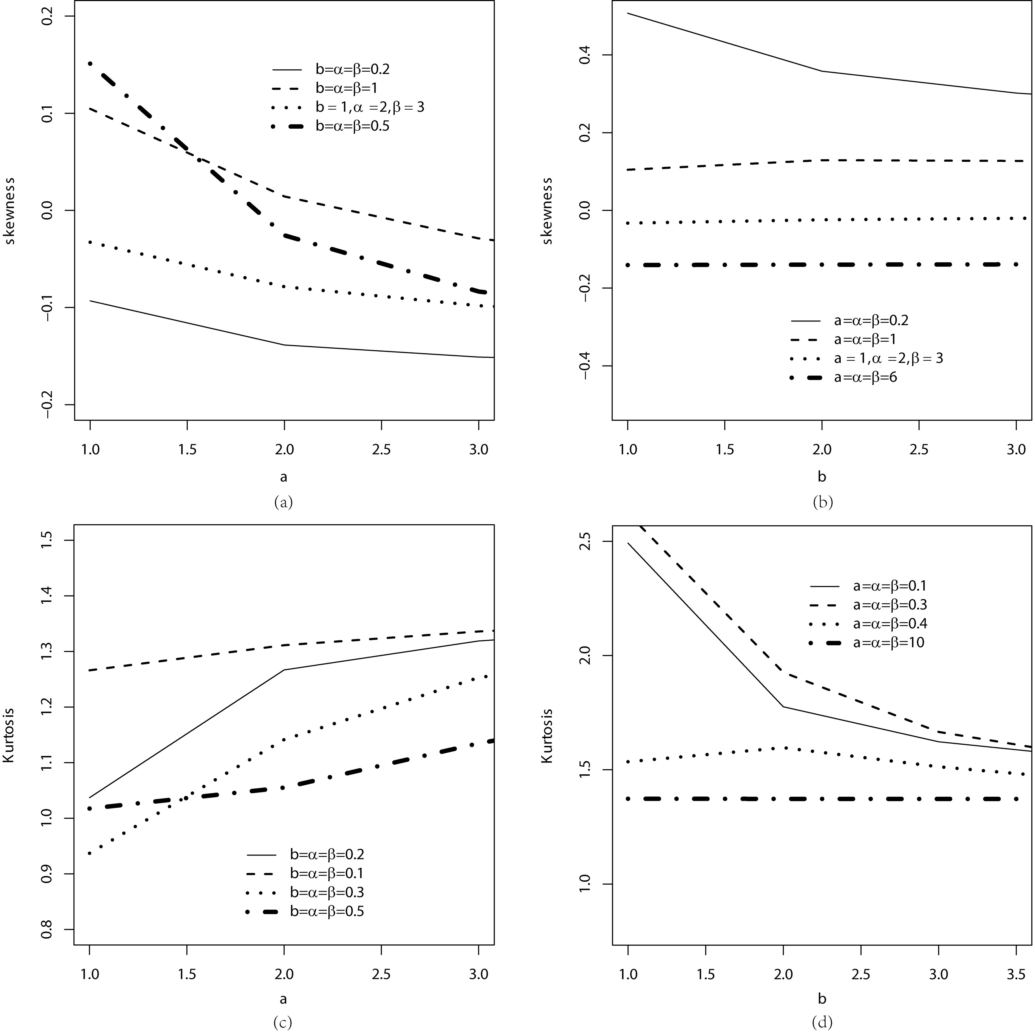
Figure 4a and b display some plots of the Bowley’s skewness of the MOE-FW distribution as functions of $a$ and $b$ for selected parameter values. Figure 4c and d do the same for Moors’ kurtosis. We obtain positive and negative skewness but only positive kurtosis.

Figure 4.

Skewness and kurtosis of the MOE-FW distribution for some parameter values.

3.2 Moments

In this section, we obtain the ordinary and incomplete moments of $T$ from the moments of the random variable $Y_{k+1}$ having the exp-G $(k+1)$ distribution.

.

For a random variable $T$ having density Eq. (7), the $n$ th ordinary moment of $T$ follows from Eq. (12) as

$\displaystyle\mu^{\prime}_{n}=E(T^{n})=\sum_{k=0}^{\infty}w_{k+1}\,E(Y_{k+1}^{% n})=\sum_{k=0}^{\infty}(k+1)w_{k+1}\,\tau_{n,k},$

where $w_{k+1}$ is given in Section 3 and $\tau_{n,k}=\int_{-\infty}^{\infty}t^{n}\,g(t)\,G(t)^{k}\,dt=\int_{0}^{1}Q_{G}^% {n}(u)\,u^{k}\,du$ .

Expressions for moments of some exp-G distributions (under special baselines) are given in Nadarajah and Kotz (2006).

.

The $n$ th incomplete moment of $T$ , say $m_{n}(y)=\int_{0}^{y}t^{n}\,f(t)dt$ , can be obtained from Eq. (12) as

$\displaystyle m_{n}(y)=\sum^{\infty}_{k=0}w_{k+1}\,\int_{0}^{y}t^{n}\,h_{k+1}(% t)=\sum_{k=0}^{\infty}(k+1)\,w_{k+1}\,\int_{0}^{G(y)}Q_{G}^{n}(u)\,u^{k}du.$

3.3 Generating function

In this section, we obtain the moment generating function (mgf) of $T$ .

.

If $T$ follows the MOE-G distribution, its mgf, say $M(s)=E[\exp(s\,T)]$ , is obtained from Eq. (12) as

$\displaystyle M(s)=\sum_{k=0}^{\infty}w_{k+1}\,\,M_{k+1}(s)=\sum_{k=0}^{\infty% }(k+1)w_{k+1}\,\rho(s,k),$

where $M_{k+1}(s)$ is the mgf of $Y_{k+1}$ and

$\displaystyle\rho(s,k)=\int_{-\infty}^{\infty}{\rm e}^{sx}\,g(x)\,G(x)^{k}\,dx% =\int_{0}^{1}\exp\left\{t\,Q_{G}(u)\right\}\,u^{k}du.$

4. Maximum likelihood

Let $T_{i}$ ( $i=1,\ldots,n$ ) be a random variable following Eq. (7) and $\bm{\theta}=(a,b,\alpha,\beta)^{\top}$ be the parameter vector. The data encountered in survival analysis and reliability studies are often censored. A very simple random censoring mechanism that is often realistic is one in which each individual $i$ is assumed to have a lifetime $T_{i}$ and a censoring time $C_{i}$ , where $T_{i}$ and $C_{i}$ are independent random variables. Suppose that the data consist of $n$ independent observations $t_{i}=\text{min}(T_{i},C_{i})$ for $i=1,\ldots,n$ . The distribution of $C_{i}$ does not depend on any of the unknown parameters of $T_{i}$ . Parametric inference for such data is usually based on likelihood methods and asymptotic theory. The censored log-likelihood for $\bm{\theta}$ is given by

$\displaystyle\ell(\bm{\theta})=r\log(a\,b)+\sum_{i\in D}\log(\alpha+\beta/t_{i% }^{2})+\sum_{i\in D}[\alpha\,t_{i}+\beta/t_{i}-\kappa_{\alpha\beta}(t_{i})]-(b% -1)\sum_{i\in D}\kappa_{\alpha\beta}(t_{i})-2\sum_{i\in D}\log\{1-(1-a)\exp[-b% \,\kappa_{\alpha\beta}(t_{i})]\}+\sum_{i\in C}\log\{a\exp[-b\,\kappa_{\alpha% \beta}(t_{i})]\}-\sum_{i\in C}\log\{1-(1-a)\exp[-b\,\kappa_{\alpha\beta}(t_{i}% )]\},$ (14)

where $\kappa_{\alpha\beta}(t_{i})=\exp(\alpha\,t_{i}-\beta/t_{i})$ , $r$ is the number of failures, and $D$ and $C$ denote the uncensored and censored sets of observations, respectively. For real-valued random variables there is no censored set of observations and hence the censored set $C$ must be removed from this function and from the quantities presented below.

The score functions for the model parameters $U_{a}(\bm{\theta})$ , $U_{b}(\bm{\theta})$ , $U_{\alpha}(\bm{\theta})$ and $U_{\beta}(\bm{\theta})$ can be obtained from the authors upon request.

The MLE $\widehat{\bm{\theta}}=(\hat{a},\hat{b},\hat{\alpha},\hat{\beta})^{\top}$ of $\bm{\theta}=(a,b,\alpha,\beta)^{\top}$ can be obtained from the nonlinear likelihood equations $U_{a}(\bm{\theta})=$ 0, $U_{b}(\bm{\theta})=$ 0, $U_{\alpha}(\bm{\theta})=$ 0 and $U_{\beta}(\bm{\theta})=$ 0. They cannot be solved analytically and iterative techniques such as the Newton-Raphson type algorithms can be used to find $\widehat{\bm{\theta}}$ numerically. We may employ the R software and the NLMixed procedure in SAS.

For interval estimation and hypothesis tests on the model parameters, we obtain the 4 $\times$ 4 observed information matrix $\bm{J}(\bm{\theta})$ numerically since the expected information matrix is very complicated and requires numerical integration.

Under standard regularity conditions, we have $\sqrt{n}(\widehat{\bm{\theta}}-\bm{\theta})\lx@stackrel{{\scriptstyle a}}{{% \sim}}{\cal{N}}_{4}(\bm{0},\bm{K}(\bm{\theta})^{-1})$ , where $\lx@stackrel{{\scriptstyle a}}{{\sim}}$ means approximately distributed and $\bm{K}(\bm{\theta})$ is the unit expected information matrix. The asymptotic behavior remains valid if $\bm{K}(\bm{\theta})=\lim_{n\to\infty}n^{-1}\bm{J}(\bm{\theta})$ , where the observed information matrix $\bm{J}(\bm{\theta})$ is replaced by the average sample information matrix evaluated at $\widehat{\bm{\theta}}$ , that is, $n^{-1}\bm{J}(\widehat{\bm{\theta}})$ . The multivariate normal ${\cal{N}}_{4}(\bm{0},n^{-1}\bm{J}(\widehat{\bm{\theta}})^{-1})$ distribution can be used to construct approximate confidence intervals for the model parameters.

Further, we can compute the maximum values of the unrestricted and restricted log-likelihoods to construct likelihood ratio (LR) statistics for testing some sub-models of the MOE-G family. In other words, we may use the LR statistic to check if the fit of the proposed family is statistically “superior” to the fit of the baseline distribution for a given data set. For example, the test of the null hypothesis ${\cal{H}}_{0}$ : $b=$ 1 against ${\cal{H}}_{1}$ : $b\neq 1$ is equivalent to compare the MOE-FW and MO-FW distributions.

4.1 Simulation study of the proposed model

In this section, we investigate the finite sample performance of the MLEs in the MOE-FW distribution by varying the true parameter vector and the sample size $n$ . We perform a Monte Carlo simulation study (with $1,000$ replications) using the R software to verify some first-order asymptotic properties of the MLEs.

We measure the accuracy of the MLEs $\hat{a}$ , $\hat{b}$ , $\hat{\alpha}$ and $\hat{\beta}$ of the MOE-FW parameters by setting $a=$ 0.25, $b=$ 0.10, $\alpha=$ 0.60 and $\beta=$ 0.50, under the mechanism of random censoring on the right, for censoring percentages (0%, 10% and 20%) and $n=$ 80, 200 and 500. For each parametric point, we calculate the average estimates (AEs) of the MLEs, the biases of the estimates and the mean squared errors (MSEs). The figures in Table 2 reveal that the AEs become closer to the true parameter values and the biases tend to zero when $n$ increases. They also indicate that the MSEs of the MLEs of the model parameters decay toward zero when $n$ increases as usually expected under first-order asymptotic theory. These facts prove empirically that the first-order asymptotic properties of the MLEs are satisfied for the MOE-FW distribution and support the asymptotic normal distribution as an adequate approximation to the finite sample distribution of these estimates.

Table 1
Simulations for the MOE-FW model

$n$	Parameter	AE	Bias	MSE	AE	Bias	MSE	AE	Bias	MSE
		0% censored			10% censored			20% censored
80	$a$	0.621	0.371	0.285	0.918	0.668	5.454	1.006	0.756	5.793
	$b$	0.247	0.147	0.039	0.307	0.207	0.116	0.338	0.238	0.162
	$\alpha$	0.498	$-$ 0.101	0.015	0.473	$-$ 0.126	0.023	0.465	$-$ 0.135	0.027
	$\beta$	0.523	0.023	0.013	0.518	0.018	0.015	0.525	0.025	0.017
200	$a$	0.444	0.194	0.098	0.585	0.335	0.546	0.826	0.576	4.235
	$b$	0.181	0.081	0.016	0.229	0.129	0.040	0.279	0.179	0.088
	$\alpha$	0.543	$-$ 0.056	0.007	0.514	$-$ 0.085	0.013	0.489	$-$ 0.111	0.019
	$\beta$	0.511	0.011	0.004	0.514	0.014	0.005	0.514	0.014	0.007
500	$a$	0.317	0.067	0.023	0.411	0.161	0.069	0.537	0.287	0.256
	$b$	0.131	0.031	0.004	0.165	0.065	0.011	0.215	0.115	0.037
	$\alpha$	0.581	$-$ 0.018	0.002	0.554	$-$ 0.046	0.005	0.525	$-$ 0.075	0.011
	$\beta$	0.508	0.008	0.001	0.513	0.013	0.002	0.506	0.006	0.002

Table 2

Simulations for the MOE-FW regression model

$n$	Parameter	AE	Bias	MSE	AE	Bias	MSE	AE	Bias	MSE
		0% censored			10% censored			20% censored
80	$\gamma_{10}$	$-$ 1.110	0.439	0.412	$-$ 1.105	0.444	0.429	$-$ 1.115	0.434	0.468
	$\gamma_{11}$	0.268	0.068	0.101	0.267	0.067	0.125	0.235	0.035	0.769
	$\gamma_{20}$	0.640	0.040	0.060	0.656	0.056	0.062	0.651	0.051	0.069
	$\gamma_{21}$	$-$ 1.081	$-$ 0.031	0.048	$-$ 1.075	$-$ 0.025	0.047	$-$ 1.084	$-$ 0.034	0.054
	$a$	1.211	$-$ 0.138	4.048	1.115	$-$ 0.235	3.922	1.225	$-$ 0.124	5.018
	$b$	1.211	$-$ 0.788	1.758	1.180	$-$ 0.819	1.775	1.205	$-$ 0.794	1.796
200	$\gamma_{10}$	$-$ 1.339	0.210	0.215	$-$ 1.323	0.226	0.242	$-$ 1.337	0.212	0.255
	$\gamma_{11}$	0.243	0.043	0.041	0.254	0.054	0.048	0.238	0.038	0.060
	$\gamma_{20}$	0.613	0.013	0.032	0.612	0.012	0.031	0.621	0.021	0.030
	$\gamma_{21}$	$-$ 1.054	$-$ 0.004	0.018	$-$ 1.055	$-$ 0.005	0.019	$-$ 1.063	$-$ 0.013	0.018
	$a$	1.390	0.040	2.134	1.377	0.027	2.240	1.373	0.023	2.212
	$b$	1.609	$-$ 0.390	1.137	1.587	$-$ 0.412	1.222	1.609	$-$ 0.391	1.226
500	$\gamma_{10}$	$-$ 1.458	0.091	0.088	$-$ 1.447	0.102	0.102	$-$ 1.419	0.130	0.135
	$\gamma_{11}$	0.198	$-$ 0.001	0.017	0.213	0.013	0.018	0.223	0.023	0.024
	$\gamma_{20}$	0.611	0.011	0.014	0.609	0.009	0.013	0.608	0.008	0.014
	$\gamma_{21}$	$-$ 1.052	$-$ 0.002	0.007	$-$ 1.055	$-$ 0.005	0.005	$-$ 1.056	$-$ 0.006	0.006
	$a$	1.376	0.026	0.860	1.362	0.012	0.928	1.342	$-$ 0.007	0.993
	$b$	1.827	$-$ 0.172	0.545	1.795	$-$ 0.204	0.619	1.747	$-$ 0.252	0.740

5. The MOE-FW regression model with two structures for censored data

Regression models can be defined in different forms in survival analysis. Among them, the location-scale regression model is distinguished since it is frequently used in clinical trials. In this section, we propose a parametric regression model based on the MOE-FW distribution with two systematic structures for censored data as a feasible alternative to the location-scale regression model. Considering that the MOE-FW and MO-FW regression models are nested models, the LR statistic can be used to discriminate between these models. We consider a classic analysis for the new regression model.

Regression analysis of lifetimes involves specifications for the distribution of a lifetime, $T$ , given a vector of covariates denoted by ${\bf v}=(v_{1},\cdots,v_{p})^{T}$ . The main aim of the systematic structures is to allow the parameters depend on ${\bf v}$ . We link the parameters $\alpha$ and $\beta$ to the covariates by the log-linear structures $\alpha_{i}=\exp({\bf v}_{i}^{T}{\mbox{\boldmath$\gamma$}}_{1})$ and $\beta_{i}=\exp({\bf v}_{i}^{T}{\mbox{\boldmath$\gamma$}}_{2})$ , $i=1,\ldots,n$ , respectively, where ${\mbox{\boldmath$\gamma$}}_{1}=(\gamma_{11},\cdots,\gamma_{1p})^{T}$ and ${\mbox{\boldmath$\gamma$}}_{2}=(\gamma_{21},\cdots,\gamma_{2p})^{T}$ denote the vectors of regression coefficients and ${\bf v}_{i}^{T}=(v_{i1},\cdots,v_{ip})$ . The MOE-FW regression model, where the parameters $\alpha$ and $\beta$ depend on ${\bf v}$ . can be very useful in many practical situations.

The survival function of $T|{\bf v}$ is given by

$\displaystyle S(t|{\bf v})=\frac{a\exp[-b\,\kappa(t|{\bf v})]}{1-(1-a)\exp[-b% \,\kappa(t|{\bf v})]},$ (15)

where

$\kappa(t|{\bf v})=\exp\left[\exp\left({\bf v}^{T}{\mbox{\boldmath$\gamma$}}_{1% }\right)\,t-\frac{\exp\left({\bf v}^{T}{\mbox{\boldmath$\gamma$}}_{2}\right)}{% t}\right].$

Equation (15) is referred to as the MOE-FW regression model with two systematic structures. This regression model opens new possibilities for fitting many different types of data. Some new special cases of the MOE-FW regression model are:

•

The MO-FW regression model

For $b=$ 1, the survival function is

$\displaystyle S(t|{\bf v})=\frac{a\exp[-\,\kappa(t|{\bf v})]}{1-(1-a)\exp[-\,% \kappa(t|{\bf v})]}.$

•

The FW regression model

For $a=b=$ 1, the survival function is

$\displaystyle S(t|{\bf v})=\exp[-\kappa(t|{\bf v})].$

Consider a sample $(t_{1},{\bf v}_{1}),\ldots,(t_{n},{\bf v}_{n})$ of $n$ independent observations, where the response variable $t_{i}$ corresponds to the observed lifetime or censoring time for the $i$ th individual. We assume non-informative censoring such that the observed lifetimes and censoring times are independent. Let $D$ and $C$ be the sets of individuals for which $t_{i}$ is the lifetime or censoring, respectively. Conventional likelihood estimation techniques can be applied here. The log-likelihood function for the vector of parameters ${\mbox{\boldmath$\theta$}}=(a,b,{\mbox{\boldmath$\gamma$}}_{1}^{T},{\mbox{% \boldmath$\gamma$}}_{2}^{T})^{T}$ from model Eq. (15) has the form $l({\mbox{\boldmath$\theta$}})=\sum_{i\in F}l_{i}({\mbox{\boldmath$\theta$}})+% \sum\limits_{i\in C}l_{i}^{(c)}({\mbox{\boldmath$\theta$}})$ , where $l_{i}({\mbox{\boldmath$\theta$}})=\log[f(t_{i}|{\bf v}_{i})]$ , $l_{i}^{(c)}({\mbox{\boldmath$\theta$}})=\log[S(t_{i}|{\bf v}_{i})]$ and $f(t_{i}|{\bf v}_{i})$ and $S(t_{i}|{\bf v}_{i})$ are the density and survival functions of $T_{i}$ , respectively. The total log-likelihood function for $\theta$ is given by

$\displaystyle l({\mbox{\boldmath$\theta$}})=r\log(a\,b)+\sum_{i\in D}\log\left% [\exp({\bf v}_{i}^{T}{\mbox{\boldmath$\gamma$}}_{1})\,t_{i}+\frac{\exp({\bf v}% _{i}^{T}{\mbox{\boldmath$\gamma$}}_{2})}{t_{i}^{2}}\right]+\sum_{i\in D}\left[% \exp({\bf v}_{i}^{T}{\mbox{\boldmath$\gamma$}}_{1})\,t_{i}+\frac{\exp({\bf v}_% {i}^{T}{\mbox{\boldmath$\gamma$}}_{2})}{t_{i}}\right]-\sum_{i\in D}\kappa(t_{i% }|{\bf v}_{i})-(b-1)\sum_{i\in D}\kappa(t_{i}|{\bf v}_{i})-2\sum_{i\in D}\log% \{1-(1-a)\exp[-b\,\kappa(t_{i}|{\bf v}_{i})]\}+\sum_{i\in C}\log\{a\exp[-b\,% \kappa(t_{i}|{\bf v}_{i})]\}-\sum_{i\in C}\log\{1-(1-a)\exp[-b\,\kappa(t_{i}|{% \bf v}_{i})]\},$ (16)

where $\kappa(t_{i}|{\bf v}_{i})$ is defined in Eq. (15), and $r$ is the number of uncensored observations (failures). The MLE $\widehat{\mbox{\boldmath$\theta$}}$ of the parameter vector ${\mbox{\boldmath$\theta$}}=(a,b,{\mbox{\boldmath$\gamma$}}_{1}^{T},{\mbox{% \boldmath$\gamma$}}_{2}^{T})^{T}$ can be obtained by maximizing the log-likelihood function. We use the R software to calculate $\widehat{\mbox{\boldmath$\theta$}}$ . Confidence intervals and hypothesis tests under general regularity conditions can be conducted using the large sample distribution of $\widehat{\mbox{\boldmath$\theta$}}$ , which is multivariate normal distribution with the covariance matrix given by the inverse of the observed information matrix. More specifically, the asymptotic covariance matrix is given by ${\bf I}^{-1}({\mbox{\boldmath$\theta$}})$ with ${\bf I}({\mbox{\boldmath$\theta$}})=E[\ddot{{\bf L}}({\mbox{\boldmath$\theta$}% })]$ such that

$\ddot{{\bf L}}({\mbox{\boldmath$\theta$}})=-\bigg{\{}\frac{\partial^{2}l({% \mbox{\boldmath$\theta$}})}{\partial{\mbox{\boldmath$\theta$}}\partial{\mbox{% \boldmath$\theta$}}^{T}}\bigg{\}}.$

It is difficult to calculate the expected information matrix ${\bf I}({\mbox{\boldmath$\theta$}})$ due to the censored observations (censoring is random and noninformative), but it is possible to use minus the matrix of second derivatives of the log-likelihood, $-\ddot{{\bf L}}({\mbox{\boldmath$\theta$}})$ , evaluated at the MLE ${\mbox{\boldmath$\theta$}}=\widehat{{\mbox{\boldmath$\theta$}}}$ , which is consistent. The asymptotic normal approximation for $\widehat{{\mbox{\boldmath$\theta$}}}$ may be expressed as $\widehat{{\mbox{\boldmath$\theta$}}}^{T}\sim N_{(2p+2)}\{{\mbox{\boldmath$% \theta$}}^{T},\ddot{{\bf L}}({\mbox{\boldmath$\theta$}})^{-1}\}$ , where $-\ddot{{\bf L}}({\mbox{\boldmath$\theta$}})$ is the $(2p+2)(2p+2)$ observed information matrix.

6. Model checking

Since regression models are sensitive to the underlying model assumptions, generally performing a sensitivity analysis is strongly advisable. Cook (1986) suggested that more confidence can be put in a model which is relatively stable under small modifications. Thus, we now present two types of diagnostic analysis of global and local influence.

A first tool to perform sensitivity analysis, as stated before, is by means of global influence starting from case-deletion. Case-deletion is a common approach to study the effect of dropping the $i$ th observation from the data set. The case-deletion for the model is given by

$\displaystyle\alpha_{l}=\exp({\bf v}_{l}^{T}{\mbox{\boldmath$\gamma$}}_{1})\ % \ \text{and}\ \ \beta_{l}=\exp({\bf v}_{l}^{T}{\mbox{\boldmath$\gamma$}}_{2}),% \ \ l=1,\ldots,n,l\neq i.$ (17)

In the following, a quantity with subscript “ $(i)$ ” means the original quantity with the ith observation deleted. For model Eq. (17), the log-likelihood function of $\theta$ is denoted by $l_{(i)}({\mbox{\boldmath$\theta$}})$ . Let $\hat{{\mbox{\boldmath$\theta$}}}_{(i)}=(\hat{a}_{(i)},\hat{b}_{(i)},\hat{{% \mbox{\boldmath$\gamma$}}}_{1(i)}^{T},\hat{{\mbox{\boldmath$\gamma$}}}_{2(i)}^% {T})^{T}$ be the MLE of $\theta$ from maximizing $l_{(i)}({\mbox{\boldmath$\theta$}})$ . To assess the influence of the ith case on the MLE $\hat{{\mbox{\boldmath$\theta$}}}=(\hat{a},\hat{b},\hat{{\mbox{\boldmath$\gamma% $}}_{1}},\hat{{\mbox{\boldmath$\gamma$}}_{2}})^{T}$ , the basic idea is to compare the difference between $\hat{{\mbox{\boldmath$\theta$}}}_{(i)}$ and $\hat{{\mbox{\boldmath$\theta$}}}$ . If deletion of an observation seriously influences the estimates, more attention should be paid to that observation. Hence, if $\hat{{\mbox{\boldmath$\theta$}}}_{(i)}$ is far from $\hat{{\mbox{\boldmath$\theta$}}}$ , then the ith observation is regarded as an influential case. A first measure of the global influence is defined as the standardized norm of $\hat{{\mbox{\boldmath$\theta$}}}_{(i)}-\hat{{\mbox{\boldmath$\theta$}}}$ (generalized Cook distance) given by

$\displaystyle\textit{GD}_{i}({\mbox{\boldmath$\theta$}})=(\hat{{\mbox{% \boldmath$\theta$}}}_{(i)}-\hat{{\mbox{\boldmath$\theta$}}})^{T}\big{[}\ddot{{% \bf L}}({\mbox{\boldmath$\theta$}})\big{]}^{-1}(\hat{{\mbox{\boldmath$\theta$}% }}_{(i)}-\hat{{\mbox{\boldmath$\theta$}}}).$

Another alternative is to assess the values $\textit{GD}_{i}(a,b)$ , $\textit{GD}_{i}({\mbox{\boldmath$\gamma$}}_{1})$ and $\textit{GD}_{i}({\mbox{\boldmath$\gamma$}}_{2})$ . Such values reveal the influence of the ${\it i}$ th observation on the estimates of $a, b$ , ${\mbox{\boldmath$\gamma$}}_{1}$ and ${\mbox{\boldmath$\gamma$}}_{2}$ , respectively. Another popular measure of the difference between $\hat{{\mbox{\boldmath$\theta$}}}_{(i)}$ and $\hat{{\mbox{\boldmath$\theta$}}}$ is the likelihood distance

$\displaystyle\textit{LD}_{i}({\mbox{\boldmath$\theta$}})=2\Big{\{}l(\hat{{% \mbox{\boldmath$\theta$}}})-l(\hat{{\mbox{\boldmath$\theta$}}}_{(i)})\Big{\}}.$

For residual analysis, we compare two residuals to assess departures from the error assumptions and to detect outliers in the MOE-FW regression model with censored observations. In the literature, various residuals were investigated in this sense. See, for example, Collett (2003). In the context of survival analysis, the deviance residuals have been more widely used because they take into account the information of censored times (Silva et al., 2011). Thus, the plot of the deviance residuals versus the observed times provides a way to verify the adequacy of the fitted model and to detect atypical observations.

The deviance residual can be expressed as

$\displaystyle r_{D_{i}}=\left\{\begin{array}[]{ll}\text{sign}(\hat{r}_{M_{i}})% \left\{-2\left[1+\log[\hat{S}(t_{i};\widehat{{\mbox{\boldmath$\theta$}}})]+% \log\{-\log[\hat{S}(t_{i};\widehat{{\mbox{\boldmath$\theta$}}})]\}\right]% \right\}^{1/2}&\text{if}\quad\delta_{i}=1,\\ \text{sign}(\hat{r}_{M_{i}})\{-2\log[\hat{S}(t_{i};\widehat{{\mbox{\boldmath$% \theta$}}})]\}^{1/2}&\text{if}\quad\delta_{i}=0,\end{array}\right.$ (18)

where

$\displaystyle\hat{S}(t_{i};\widehat{{\mbox{\boldmath$\theta$}}})=\frac{\hat{a}% \exp[-\hat{b}\,\hat{\kappa}(t_{i}|{\bf v}_{i})]}{1-(1-\hat{a})\exp[-\hat{b}\,% \hat{\kappa}(t_{i}|{\bf v}_{i})]},\hat{\kappa}(t_{i}|{\bf v}_{i})=\exp\left[% \exp\left({\bf v}_{i}^{T}\widehat{{\mbox{\boldmath$\gamma$}}}_{1}\right)\,t_{i% }-\frac{\exp\left({\bf v}_{i}^{T}\widehat{{\mbox{\boldmath$\gamma$}}}_{2}% \right)}{t_{i}}\right],$

$\hat{r}_{M_{i}}=\delta_{i}+\log[\hat{S}(t_{i};\widehat{{\mbox{\boldmath$\theta% $}}})]$ is the martingale residual and $\text{sign}(\cdot)$ is a function that leads to the values $+1$ if the argument is positive and $-1$ if the argument is negative.

6.1 Simulation study of the regression model

A simulation study is carried out to investigate the behavior of the empirical distribution of the deviance component residuals, and also to assess the AEs, MSEs and biases of the MLEs of the parameters in the MOE-FW regression model with censored data.

We simulate 1,000 samples by taking the true parameter values as $\gamma_{10}=$ $-$ 1.55, $\gamma_{11}=$ 0.20, $\gamma_{20}=$ 0.60, $\gamma_{21}=$ $-$ 1.05, $a=$ 1.35 and $b=$ 2.0, and under the mechanism of random censoring on the right, for censoring percentages (0%, 10% and 20%). The lifetimes, denoted by $t_{1},\cdots,t_{n}$ , are generated from the MOE-FW regression model Eq. (15), where $\alpha=\exp(\gamma_{10}+\gamma_{11}v_{1})$ and $\beta=\exp(\gamma_{20}+\gamma_{21}v_{1})$ . The survival times are generated from the following algorithm adapted for censored data:

1.
Generate $u\sim$ Uniform(0,1).
2.
Generate $v_{1}\sim$ Binomial(1,0.5) by considering two groups (0 and 1).
3.
Generate $c\sim$ Uniform(0, $\tau$ ), where $\tau$ denotes the proportion of censored observations.
4.
Use steps 1 and 2 to compute the observations $t^{}_{i}$ from Eq. (13).
5.
Set $t_{i}=\text{min}(t^{}_{i},c)$ .
6.
Define a vector $\delta$ of dimension $n$ which receives one if ( $t^{*}_{i}\leqslant c)$ and zero otherwise.

Table 2 gives the AEs, biases and MSEs of the MLEs of $\gamma_{10}$ , $\gamma_{11}$ , $\gamma_{20}$ , $\gamma_{21}$ , $a$ and $b$ calculated from the simulations. We note that the AEs tend to be closer to the true parameter values and the biases and MSEs decay toward zero when the sample size $n$ increases as expected under first-order asymptotic theory. So, the asymptotic normal distribution provides an adequate approximation to the finite sample distribution of the estimates.

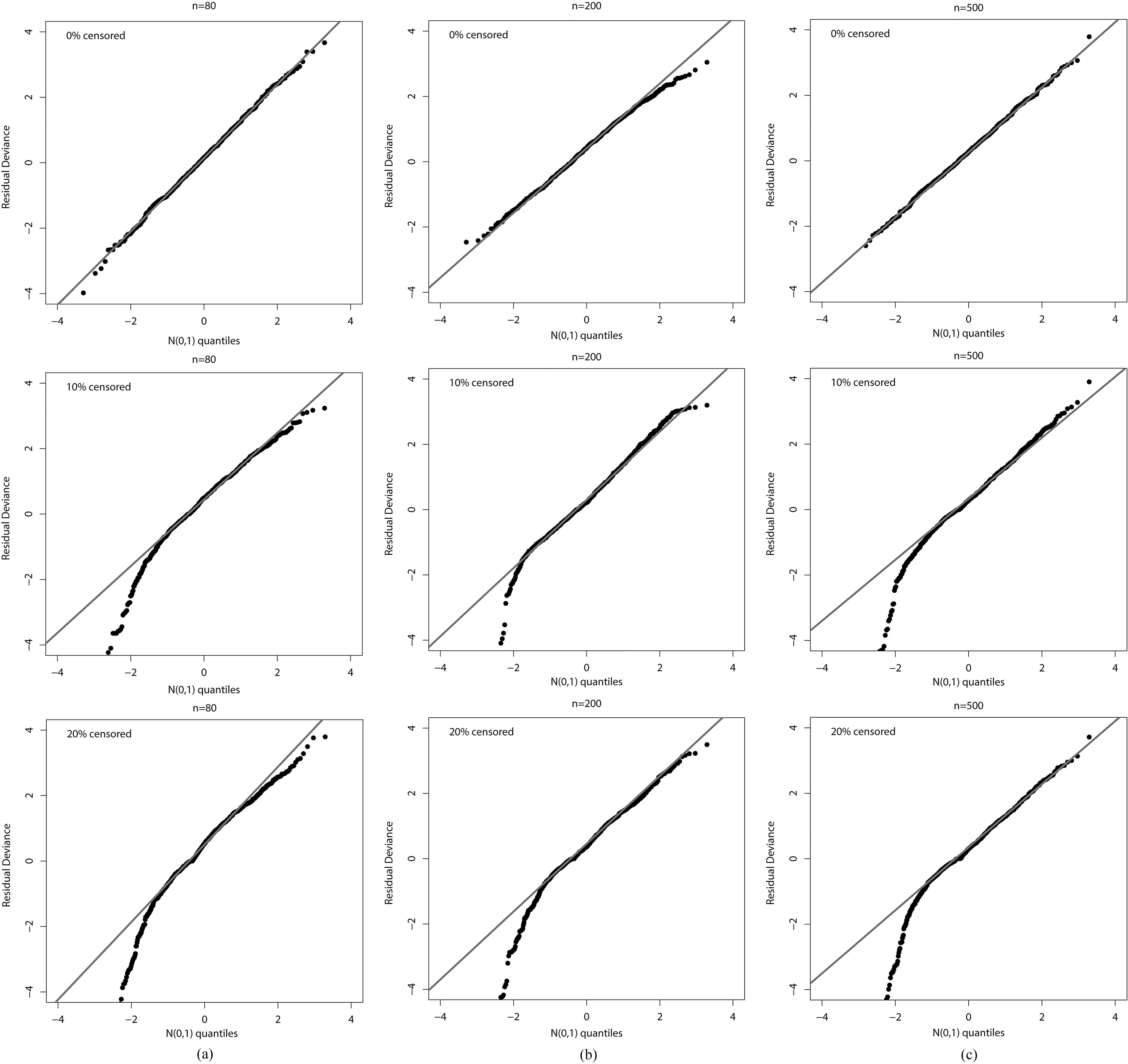
Further, we display the plots of the ordered residuals versus the expected values of the order statistics of the standard normal distribution in Fig. 5. This type of graphic is known as the Q-Q plot and serves to assess the departure from the normality assumption of residuals. Hence, the following conclusions on the empirical distribution of the deviance residuals come from the plots in Fig. 5: i) It agrees with the standard normal distribution; ii) It tends to the standard normal distribution more rapidly when the censoring percentage decreases; iii) It becomes closer to the normal distribution when the sample size increases.

Figure 5.
QQ-plots for the deviance residuals $(r_{D_{i}})$ in the MOE-FW regression model. (a) $n=$ 80 and (0%, 10% and 20%) censored. (b) $n=$ 200 and (0%, 10% and 20%) censored. (c) $n=$ 500 and (0%, 10% and 20%) censored.

7. Applications

We provide two applications of the results derived in the previous sections by means of real data sets. We calculate the MLEs and their standard errors (SEs) (given in parentheses) of the model parameters and the values of the Akaike Information Criterion (AIC), Bayesian Information Criterion (BIC), Cramér-von Mises ( $W^{*}$ ) and Anderson Darling ( $A^{*}$ ) statistics for the fitted models. The lower the values of these measures, the better the fit. For all distributions, the model parameters are estimated by maximum likelihood using the BFGS algorithm. For the first application, we adopt the AdequacyModel script, whereas for the second we use the optim function in the R software.

In the first application, we prove empirically that the MOE-FW distribution outperforms the MO-FW and FW distributions and other non-nested distributions defined in the sequel. We consider the Weibull distribution with scale $\alpha>$ 0 and shape $\tau>$ 0. The cdf of the exponentiated Flexible Weibull (EFW) distribution is given by

$\displaystyle F(t)=\Biggl{[}1-\exp\Biggl{\{}-\exp\left(\mu t-\frac{\sigma}{t}% \right)\Biggl{\}}\Biggl{]}^{\varphi},\,\,t>0,$

where $\mu>$ 0, $\sigma>$ 0 and $\varphi>$ 0 are shape parameters.

The cdf of the Kumaraswamy inverse Flexible Weibull (Kw-IFW) (Al Abbasi, 2016) is

$\displaystyle F(t)=1-\Biggl{\{}1-\Biggl{[}\exp\left(-\exp\left(\frac{\mu}{t}-% \sigma t\right)\right)\Biggl{]}^{\lambda}\Biggl{\}}^{\varphi},\,\,t>0,$

where $\mu>$ 0, $\sigma>$ 0 and $\varphi$ and $\lambda$ are positive shape parameters. The inverse Flexible Weibull extension (IFW) distribution follows by setting $\varphi=$ 1 and $\lambda=$ 1.

The cdf of the generalized Flexible Weibull extension (GFWEx) distribution (with four parameters $\mu>$ 0, $\sigma>$ 0, $\varphi>$ 0 and $\lambda>$ 0) (Ahmad & Iqba, 2017) is given by

$\displaystyle F(t)=1-\exp\Biggl{\{}-\lambda\Biggl{[}\exp\left(\mu t-\frac{% \sigma}{t}\right)\Biggl{]}^{\varphi}\Biggl{\}},\,\,t>0.$

In the second application, we compare the MOE-FW and FW regression models.

7.1 Application 1: Failure time data

The data set is reported in Murthy et al. (2004, Table 11.2). The results from some fitted distributions to these data are listed in Table 3. The four statistics are in favor of the MOE-FW distribution. The smallest values of these criteria correspond to the proposed distribution, which could be chosen as the best model in this case.

Table 3
MLEs and their SEs (in parentheses) of the model parameters and statistical measures for complete failure time data

Model	$a$	$b$	$\alpha$	$\beta$	AIC	BIC	$W^{*}$	$A^{*}$
MOE-FW	80.190	4.194	0.063	0.128	212.8	220.5	0.076	0.547
	(0.001)	(0.000)	(0.001)	(0.002)
MO-FW	2.583	1	0.157	0.196	217.7	223.5	0.171	1.077
	(0.702)	( $-$ )	(0.016)	(0.052)
FW	1	1	0.135	0.285	227.8	231.6	0.248	1.665
	( $-$ )	( $-$ )	(0.016)	(0.059)
	$\lambda$	$\varphi$	$\mu$	$\sigma$
Kw-IFW	0.957	0.104	0.033	3.264	211.8	219.4	0.114	0.635
	(0.019)	(0.014)	(0.015)	(0.003)
IFW	1	1	0.049	0.354	224.2	228.0	0.157	1.008
	( $-$ )	( $-$ )	(0.009)	(0.051)
GFWEx	0.499	0.1521	1.353	1.366	221.6	229.2	0.190	1.195
	(0.024)	(0.000)	(0.001)	(0.000)
EFW		2.343	0.156	0.089	220.9	226.6	0.197	1.196
		(0.526)	(0.016)	(0.036)
	$\alpha$	$\tau$
Weibull	2.725	0.881			209.0	212.8	0.096	0.547
	(0.460)	(0.099)

Formal tests for the extra parameters $a$ and $b$ in the proposed distribution can be based on LR statistics as given in Table 4. We reject the null hypotheses in the two tests in favor of the MOE-FW distribution. The rejection is extremely highly significant and gives clear evidence of the potentiality of the shape parameters $a$ and $b$ when modeling real data. The plots of the fitted MOE-FW, Kw-IFW and Weibull densities are displayed in Fig. 6.

Table 4

LR tests for complete failure time data

Models	Hypotheses	Statistic $w$	$p$ -value
MOE-FW vs MO-FW	$H_{0}:b=$ 1 vs $H_{1}:H_{0}\,\text{is\,false}$	6.98	0.0082
MOE-FW vs FW	$H_{0}:a=b=$ 1 vs $H_{1}:H_{0}\,\text{is\,false}$	19.0	0.00007

The TTT plot for the current data in Fig. 6a reveals a bathtub shaped hrf and, therefore, indicates the appropriateness of the MOE-FW distribution for these data. The plots of the histogram and the fitted MOE-FW, Kw-IFW and Weibull densities are displayed in Fig. 6b. The plots of the empirical cdf and estimated cdfs are displayed in Fig. 6c. We conclude from these plots that the MOE-FW distribution is very suitable to these data. The Weibull model is less efficient only in terms of the $W^{*}$ statistic, but the plots indicate that it does not provide a good fit to the current data.

Figure 6.

(a) TTT plot for the complete failure time data. (b) Estimated densities of the MOE-FW, Kw-IFW and Weibull distributions for the complete failure time data. (c) Estimated cdfs of the MOE-FW, Kw-IFW and Weibull distributions for the complete failure time data.

7.2 Application 2: Regression model for multiple-censored relay data

We present data on a production relay and on a proposed design change ( $n=$ 35) with 14% of censored data. Engineering experience suggested that the lifetime follows the Weibull distribution. Engineering sought to compare the production and proposed designs over the range of test currents. These data are also reported in Nelson (2003). We adopt the MOE-FW regression model to analyze these data. The variables involved in the study are:

•
$x_{i}$ – observed thousands of cycles;
•
$\delta_{i}$ – censoring indicator (0 $=$ censoring, 1 $=$ lifetime observed);
•
$v_{i}$ – production of levels (16 amps, 26 amps and 28 amps) is defined by dummy variables: 16 amps ( $v_{i1}=$ 1 and $v_{i2}=$ 0), 26 amps ( $v_{i1}=$ 0 and $v_{i2}=$ 1) and 28 amps ( $v_{i1}=$ 0 and $v_{i2}=$ 0).

Table 5
GD, AIC and BIC statistics for comparing the MOE-FW and FW models to the multiple-censored relay data

Model GD AIC BIC

MOE-FW 371.4 387.4 399.8

FW 397.8 409.8 419.1

Table 6
MLEs, SEs and $p$ -values for regression model fitted to the multiple-censored relay data

Parameter Estimate SE $p$ -value

$a$ 0.426 0.700 –

$b$ 0.840 1.878 –

$\gamma_{10}$ 5.160 0.832 $<$ 0.001

$\gamma_{11}$ $-$ 0.903 0.395 0.028

$\gamma_{12}$ 0.170 0.651 0.795

$\gamma_{20}$ 5.820 0.407 $<$ 0.001

$\gamma_{21}$ 0.635 0.330 0.052

$\gamma_{22}$ $-$ 0.082 0.459 0.859

Figure 7.
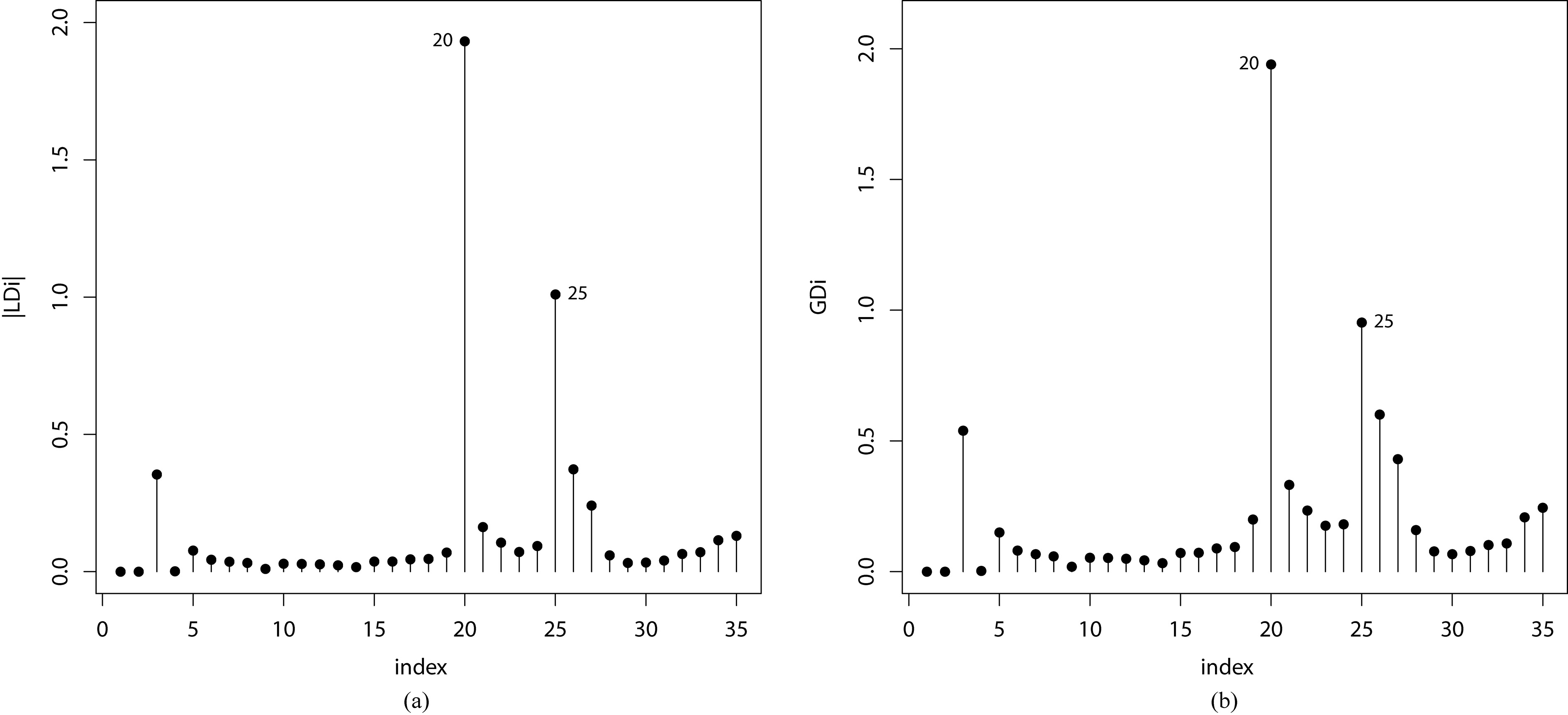
(a) Index plot of $\textit{LD}_{i}({\mbox{\boldmath$\theta$}})$ for $\theta$ on the relay data. (b) Index plot of $\textit{GD}_{i}({\mbox{\boldmath$\theta$}})$ for $\theta$ on the relay data.

We consider the following systematic structures:

$\displaystyle\alpha=\exp(\gamma_{10}+\gamma_{11}v_{i1}+\gamma_{12}v_{i2}),% \beta=\exp(\gamma_{20}+\gamma_{21}v_{i1}+\gamma_{22}v_{i2}),i=1,\ldots,35.$

We maximize the log-likelihood function Eq. (16) and obtain the MLEs of the model parameters using the R software. We take for initial values the estimates from the fitted Weibull regression model. The values of the global deviance (GD), AIC and BIC to compare the MOE-FW and FW regression models are given in Table 5. The MOE-FW regression model outperforms the FW model irrespective of the criteria and it can be used effectively in the analysis of these data.

Figure 8.
(a) Index plot of the deviance residuals for the relay data and (b) Normal probability plot for the deviance component residuals with envelope from the fitted MOE-FW regression model to relay data.

Figure 9.
(a) Estimated survival function for the MOE-FW regression model and the empirical survival. (b) The fitted hazard functions for the levels 16, 26 and 28 amps.

Further, we give the parameter estimates, SEs and significance of the MLEs in Table 6. The figures in this table indicate that there is evidence that the presence of the only covariate $v_{1}$ is significant at 5% level of significance, i.e., there is a significant difference of the level 16 amps with respect to the level 26 amps.
7.3 Checking the model

Model	GD	AIC	BIC
MOE-FW	371.4	387.4	399.8
FW	397.8	409.8	419.1

Parameter	Estimate	SE	$p$ -value
$a$	0.426	0.700	–
$b$	0.840	1.878	–
$\gamma_{10}$	5.160	0.832	$<$ 0.001
$\gamma_{11}$	$-$ 0.903	0.395	0.028
$\gamma_{12}$	0.170	0.651	0.795
$\gamma_{20}$	5.820	0.407	$<$ 0.001
$\gamma_{21}$	0.635	0.330	0.052
$\gamma_{22}$	$-$ 0.082	0.459	0.859

We use the R software to calculate the case-deletion measures $\textit{GD}_{i}({\mbox{\boldmath$\theta$}})$ and $\textit{LD}_{i}({\mbox{\boldmath$\theta$}})$ given in Section 6. The index plots of these influence measures are displayed in Fig. 7. These plots reveal that the cases $\sharp$ 20 and $\sharp$ 25 are possible influential observations.

We perform the residual analysis by plotting in Fig. 8a the deviance component residuals $r_{D_{i}}$ (see Section 6) against the index of the observations. Figure 8a shows some large residuals (observations $\sharp$ 3 and $\sharp$ 25), although Fig. 8b gives the normal probability plot with generated envelope supporting the hypothesis that the MOE-FW regression model is very suitable for these data, since there are no observations falling outside the envelope.

In order to assess if the model is appropriate, the plots comparing the empirical and estimated survival functions for the MOE-FW regression model are given in Fig. 9a. These plots indicate that the MOE-FW regression model yields a satisfactory fit to the current data. There is a significant difference of the level 16 amps with respect to the levels 26 amps and 28 amps. We also present in Fig. 9b the fitted hazard functions. From these plots, we can note a significant different between the survival curves. However, the MOE-FW regression model yields a better fit to the current data.

8. Conclusions

We define and study a new class of distributions called the Marshall-Olkin extended-G with two extra positive parameters. We provide some mathematical properties of the new class including moments and generating function. We propose a new special distribution in this class called the MOE-Flexible Weibull (MOE-FW). The maximum likelihood method is used for estimating its model parameters. We provide a simulation study to verify the performance of the maximum likelihood estimators in terms of biases and mean squared errors. We construct a new regression model with two systematic structures based on the MOE-FW distribution. We also discuss the sensitivity of these estimators from the fitted model using global influence and deviance residuals. The usefulness of the proposed models is illustrated by means of two real data sets. They provide consistently better fits than other competitive models for these data sets. Due to recent advances in computational technology, it is worthwhile to carry out Bayesian treatments via Markov chain Monte Carlo (MCMC) sampling methods in the context of the MOE-FW regression model. Bayesian influence diagnostics can be treated via the Kullback-Leibler divergence as proposed by Cancho et al. (2010). Other extensions of the current work include, for example, a generalization of MOE-FW to multivariate settings and MOE-FW regression model with random effects and censored data.

Footnotes

Acknowledgments

We would like to thank the reviewers for their constructive comments, which helped to improve this paper substantially. This research work was supported in part by grants from Conselho Nacional de Desenvolvimento Científico e Tecnológico (CNPq) and CAPES, Brazil.

References

Alizadeh,

Tahir,

M.H.

Cordeiro,

G.M.

Zubair,

, & Hamedani,

G.G.

(2015). The Kumaraswamy Marshal-Olkin family of distributions. Journal of the Egyptian Mathematical Society, 23, 546-557.

Barreto-Souza,

Lemonte,

A.J.

, & Cordeiro,

G.M.

(2013). General results for Marshall and Olkin’s family of distributions. Anais da Academia Brasileira de Ciências, 85, 3-21.

Bebbington,

Lai,

C.D.

, & Zitikis,

(2007). A flexible Weibull extension. Reliability Engineering and System Safety, 92, 719-726.

Cancho,

V.G.

Ortega,

E.M.M.

, & Paula,

G.A.

(2010). On estimation and influence diagnostics for log-Birnbaum-Saunders Student-t regression models: Full Bayesian analysis. Journal of Statistical Planning and Inference, 140, 2486-2496.

Collett,

(1994). Modelling Survival Data in Medical Research. Chapman and Hall, London.

Cook,

R.D.

(1986). Assessment of local influence (with discussion). Journal of the Royal Statistical Society B, 48, 133-169.

Cordeiro,

G.M.

Lemonte,

A.J.

, & Ortega,

E.E.M.

(2014). The Marshall-Olkin family of distributions: Mathematical properties and new models. Journal of Statistical Theory and Practice, 8, 343-366.

Krishna,

Jose,

K.K.

, & Ristic,

(2013). Applications of Marshal-Olkin Fréchet distribution. Communications in Statistics – Simulation and Computation, 42, 76-89.

Marshall,

A.W.

, & Olkin,

(1997). A new method for adding a parameter to a family of distributions with application to the exponential and Weibull families. Biometrika, 84, 641-652.

10.

Murthy,

D.N.P.

Xie,

, & Jiang,

(2004). Weibull models, John Wiley and Sons, New Jersey.

11.

Nelson,

W.B.

(2004). Accelerated testing statistical models, test, plans and data analysis, Wiley, Hoboken, New Jersey.

12.

Nadarajah,

, & Kotz,

(2006). The exponentiated type distributions. Acta Applicandae Mathematicae, 92, 97-111.

13.

Silva,

G.O.

Ortega,

E.M.M.

, & Paula,

G.A.

(2011). Residuals for log-Burr XII regression models in survival analysis. Journal of Applied Statistics, 38, 1435-1445.

The Marshall-Olkin extended flexible Weibull regression model for censored lifetime data

Abstract

Keywords

1. Introduction

2. Marshall-Olkin extended family

.

.

.

.

3.3 Generating function

.

4. Maximum likelihood

Table 1 Simulations for the MOE-FW model

7.1 Application 1: Failure time data

Table 3 MLEs and their SEs (in parentheses) of the model parameters and statistical measures for complete failure time data

8. Conclusions

Footnotes

Acknowledgments

References

Table 1
Simulations for the MOE-FW model

Table 3
MLEs and their SEs (in parentheses) of the model parameters and statistical measures for complete failure time data