Offline fitting Markov switching model

Abstract

Markov regime switching models remain enormously popular in speech recognition, economics, finance, etc. Nonparametric segmentation in switching models without probability assignment of jump moments is in many papers by Brodsky and Darkhovsky. We model all regimes as long SCOT strings. Stochastic COntext Tree (abbreviated as SCOT) is $m$ -Markov Chain ( $m$ -MC) with every state of a string independent of the symbols in its more remote past than the context of length determined by the preceding symbols of this state. A parallel super-fast fitting and asymptotically optimal inference in a sparse SCOT model including the nonparametric homogeneity test are described in our previous papers. Our segmentation method is a combination of preliminary online change point detection with its subsequent offline Maximal Likelihood update.

Keywords

Strong mixing SCOT emissions Markov switching model change point detection maximum likelihood HMM

1. Introduction

Approximability of mixing stationary sequences by $m$ -MC with large $m$ belongs to the mathematical folklore and is widely used without rigorous definitions in the Information Theory, see Cover (2006). In view of exponential complexity of general $m$ -MC, ARMA-models were their popular surrogates until sparse memory $m$ -MC named VLMC was introduced in Rissanen (1983) for compression aims. We discuss conditions for sparse $m$ -MC approximation of strong mixing stationary sequences called Stochastic Context Trees (SCOT) in Section 2. Parameter $A$ in sparse SCOT introduced in Section 2 depends in general on accuracy of the approximation and can be arbitrarily large, even infinite, making this process not Markov. Thus, this alternative name is appropriate to VLMC (which is much wider used for a video editor). An alternative apparently less powerful and flexible model is Markov Chain of Conditional Order, see Kharin and Maltsau (2014).

The ergodicity of Markov Chains (MC) and Asymptotic Normality (AN) of additive functions of their paths has been subject of numerous studies starting from the pioneering works of Markov and Bernstein in the beginning of 20th century. Among many popular surveys – Borovkov (1998); Meyn (1993); Tutubalin (1992); Veretennikov (2000). Statistical inference for MC has become popular after Billingsley (1961); Roussas (1972). The second of these references introduced the MC Local Asymptotic Normality (LAN) following the Le Cam-Hajek asymptotic locally minimax inference theory. An elementary exposition of this theory is in Veretennikov (2000). Our Section 5 outlines a simpler straightforward LAN derivation for finite MC following (with some revisions) Tutubalin (1992); Veretennikov (2000) rather than the popular much longer CLT reduction to the more general Martingale CLT. The latter approach involves a cumbersome Poisson-like inverse problem solution which is not straightforward (Meyn (1993); Veretennikov (2000)).

Ryabko (2016) and finally Zhang (2017) established the equivalence of a perfect memory sparse SCOT to 1-MC with state space consisting of the $m$ -MC contexts which we call new alphabet $\mathcal{A}$ of cardinality $A$ . For not perfect memory sparse SCOT, its perfect memory sparse envelope also studied in Zhang (2017) plays this role, see an outline in Appendix 3. The perfect memory condition does not depend on prediction probabilities assigned to the leaves of SCOT.

A substantial part of the present paper deals with statistical properties of 1-MC. The statistical theory of SCOT cumbersome calculations requiring a sophisticated software is covered miraculously by the classical 1-MC theory with somewhat larger alphabet size $A$ under perfect memory.

Thus, by first applying UA- $m$ -MC and $\mathcal{M}$ conditions, we reduce a stationary sequence to an $m$ -MC with sparse memory structure, and reduce it further to a 1-MC with alphabet $\mathcal{A}$ .

Our statistical SCOT modeling (Ryabko, 2016; Malyutov et al., 2013) of financial data discovered a small size of the context tree, while literary texts showed the adequate number of SCOT contexts $A$ around 2000.

This application suggests a modified asymptotics for deriving AN of additive SCOT functions for moderate sample sizes. An example in Appendix 1 illustrates this phenomenon by the spectral decomposition of cyclic random walks derived in Feller (1967), pp. 377–378 and 434–435.

The large $A$ asymptotics can be studied in future by the first order Edgeworth-type expansion for the additive functions developed for IID $X_{i},i=1,\ldots,N$ , observations. The principal multiplier $(\mu_{3}/\sigma^{3})/\sqrt{N}$ of the residual term may grow with $m$ which worsens the precision of approximation. Here $\mu_{3},\sigma$ are the stationary third moment and standard deviation of $X_{i}$ respectively.

Section 8.1 justifies SCOT homogeneity testing (HT) results of Ryabko (2016) and Malyutov et al. (2013) and Section 9 HT applications in the framework of local (contiguous) alternatives theory under LAN. Testing very distant alternatives was exposed earlier in Ryabko (2016) and Malyutov et al. (2013) for an example of screening out active inputs of a multivariate regression model with colored noise using the large deviations probability results. Estimation and testing in Section 9 of transition probabilities in sliding windows is aimed at distinguishing abrupt changes in SCOT model from its small deviations.

The speed up of SCOT training of the sparse $m$ -MC with a large alphabet size or for multichannel online SCOT training prompted our novel development of a parallel implementation Malyutov and Grosu (2017) of the algorithms developed earlier in Rissanen (1983) and Mächler and Bühlmann (2004) et al., see a brief outline in Section 12.

1.1 HMM model for speech recognition

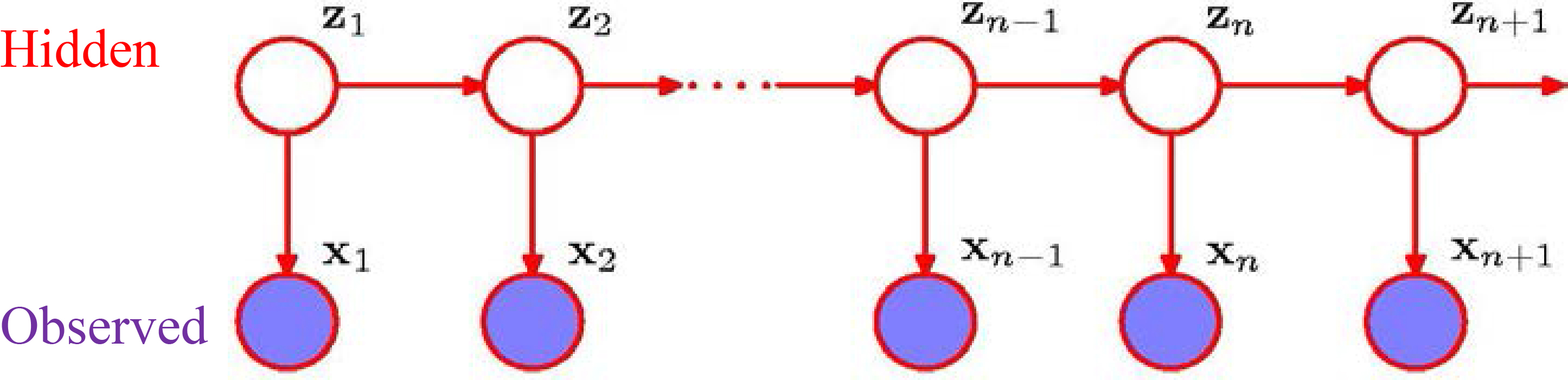
The Hidden Markov Model (HMM) is the simplest regime switching model with all regimes consisting of random strings called emissions. Emissions are INDEPENDENT (mutually and of HMM) with distribution depending on the current HMM state.

Speech is modeled (Baum et al.) as a sequence of emissions – phonems – random variables $x_{i}$ . Observed state $x_{i}$ depend only on current hidden letter of text $z_{i}$ which sequence is modeled as a Markov Chain.

We refer to $z_{i}$ as hidden states, see the Plot 1 below. Inference about the parameters of the model and hidden MC uses only the observed $x_{i},i=1,\ldots$

The fast Baum-Welsh fitting HMM parameters has been successfully applied to speech recognition Rabiner (1989). Its application to Genome modeling Durbin (1998); Yoon (2009) by assigning IID emissions to the same part of Genome seems not justified. Markov switching models generalize HMM by considering parametric regimes (Hamilton, 2008; Cappe, 2005). Nonparametric segmentation in switching models without probability assignment of jump moments is in many works by Brodsky and Darkhovsky, see Brodsky (1993). We develop a model of slow HMM with SCOT emissions (SCOT-HMM) which seems a more realistic model for Genome, economics, analysis of combined authorship of literary works, or financial time series with piecewise volatility. We discuss in Malyutov (2017, 2012) approaches to SCOT-approximation of mixing sequences enabling consideration of mixing emissions.

1.2 Slow HMM-SCOT emissions model

We call HMM $z_{i}$ SLOW, if mean time that HMM keeps staying in the same state is proportional to a large parameter $l$ in all states, while the sample size is $kl,k\to\infty$ . Emissions shown in dark in the following Fig. are modeled as STRINGS of MC over the space of contexts with transition matrix depending on the current HMM state.

.

Our HMM-SCOT model has nothing in common with VLMCHMM which analyzes independent emissions under a SCOT model for HMM Dumont (2014).

The emissions MC $x_{i}$ over the alphabet of SCOT contexts are assumed ergodic, different for all states of HMM, expectations are taken everywhere under their stationary distributions.

Our segmentation method is a superposition of preliminary online change point detection with its subsequent offline Maximal Likelihood update. The online and offline parts are nontrivial modifications of IID case in Korostelev (2011) using alternative risk function to that in Shiryaev (1978).

Figure 1.

HMM-SCOT scheme.

Appendices 2–4 outline respectively a parallel SCOT training algorithm Malyutov (2012), perfect memory and statistical simulation of the first Change Point (CP) detection.

2. Approximation by SCOT

Approximation of strong mixing sequences by $m$ -MC with large $m$ belongs to the mathematical folklore and is widely used without rigorous definitions in the Information Theory, see Cover (2006). We consider a strictly stationary process $X(t)$ over an alphabet $\cal{X}$ and discrete time: $X_{t},-\infty<t<\infty$ , with potentially infinite memory which can be approximated uniformly by an $m$ -Markov chain (UA- $m$ -MC condition).

By this we mean that for any $\varepsilon>$ 0 there exists a positive integer $m(\varepsilon)>$ 0 such that

$\displaystyle|P(X_{0}|X_{-\infty}^{-1})-P(X_{0}|X_{-m}^{-1})|<\varepsilon$

for almost every $X_{0}$ and past sequences $X_{-\infty}^{-1}$ .

.

Apparently, a uniform version of exponential memory decay absolute mixing (attributed to A.N. Kolmogorov in Volkonskii (1959)) can guarantee a uniform approximation by an $m$ -MC.

Numerous conditions of strong mixing sequences are reviewed in Bradley (2005). Assume now the UA- $m$ -MC condition of a stationary sequence $x_{-\infty}^{\infty}$ and fix $m(\varepsilon)$ of the approximating $m$ -MC which is assumed ergodic. Sequences $x_{1}^{m}$ are called $m$ -grams. Let us introduce contexts for each of $A^{m}$ different realizations $a_{1}^{m}$ of $m$ -gram.

The context to $a_{1}^{m}$ is its final part of minimal length $l(a_{1}^{m})$ such that the conditional distributions $P(X_{m+1}|x$ , $a_{m-l}^{m})$ do not depend on prefix $x$ up to joint error probability $<\varepsilon$ . This statement is described by simultaneous validity of obvious $A\times(A-1)$ double inequalities. Not occurring $m$ -grams are ignored.

To streamline introduction, we assume that there are no such $m$ -grams. Such a twice approximated stationary sequence will be called $\varepsilon$ -SCOT with small abuse of notation.

Finally, the memory spectrum $\mathcal{M}$ is the $2^{m}$ -vector of context lengths along all $2^{m}$ paths from the root to the past.

We combine all preceding developments into the following:

.

If a UA- $m$ -MC has a memory spectrum $\mathcal{M}$ , then $X_{-\infty}^{\infty}$ is an $\varepsilon$ -SCOT with the corresponding context length distribution.

We say that $X_{-\infty}^{\infty}$ has a sparse $m$ -MC representation, if the average over steady state distribution of context lengths satisfies:

$\displaystyle 2^{-m}\sum_{i=1}^{2^{m}}Em_{i}=o(2^{m}).$

Widespread sparse processes in nature phenomenon are explained by the ‘Occam razor’ or ‘Bottleneck’ popular philosophical principles.

The median, or a quantile collection, or other functions of $\mathcal{M}$ over the stationary distribution can be also used for defining sparsity.

Many examples of stationary distribution evaluation in various SCOT models are in Ryabko (2016).

We develop further asymptotic theory for fixed $A$ and large sample size and, therefore, for a finite ergodic MC assuming $\varepsilon=$ 0 in previously outlined more general approximations.

Thus, by first applying UA- $m$ -MC and $\mathcal{M}$ conditions, we have reduced a stationary sequence to an $m$ -MC with sparse memory structure, and finally reduce it further to a 1-MC with a larger alphabet $\mathcal{A}$ .

An ergodic Hidden Markov Model (HMM) is the simplest regime switching model with all B regimes consisting of sequences of random variables called emissions. We call it SLOW, if all transition probabilities to stay in the same state $b$ are $1-l^{-1}C_{b}$ , where $l$ is a large parameter and the sample size is $kl,k\to\infty$ . Emissions are modeled as independent of HMM MC over the space of contexts with transition matrix depending on the current HMM state $b,1\leqslant b\leqslant B$ .

Introduce stationary log-likelihoods $l_{i}=l(x(i-1),x(i))=\log P(x_{i}|x_{i-1})$ and entropy of SCOT( $b$ ):

$\displaystyle h(b)=\lim_{M\to\infty}M^{-1}E\left(\sum_{1}^{M}l_{i}\right).$

The emissions MC $x_{i}$ over the alphabet of SCOT contexts are assumed ergodic for every state of HMM, expectations are taken under their stationary distributions which are assumed strictly different for all $b$ .

Given a long string with a vast collection of $m$ -grams, the probability distributions can be approximated with their corresponding consistent frequencies. This allows the sparse MC consistent training dealt with in Galves (2008); Bühlmann (2004); Rissanen (1983). A version of SCOT training on a cluster of computers valid for a large alphabet $A$ , is described in our Section 8. A fitting algorithm has been proved to be consistent for mixing sequences in Rissanen (1983) and used for compression. A somewhat confusing abbreviation VLMC (which is more widely used for a video editor) has been initially chosen for SCOT. For completeness, we display in Section 2 a sketch of the Context algorithm consistency from Galves (2008) admitting horizon $O(\log N)$ and the sample size $N\to\infty$ . A popular software Bühlmann (2004) implementing the Context algorithm of Rissanen (1983) assumes a fixed horizon as $N\to\infty$ . We sketch simplifications in proving consistency under this assumption.

3. Consistency of SCOT training

$P(y,x_{M},\ldots,x_{1})$ is the joint empirical distribution of $(y=x_{0},x_{M},\ldots,x_{1})$ .

For a node $A=x_{i},\ldots,x_{1},P(y|zA)=P(y|A)/P(y|zA)=P(y,zA)/\sum_{b\in A}P(b,zA)$ is the conditional empirical distribution of $z A$ given $A$ , where $z A$ denotes the string $(z,x_{i},\ldots,x_{1})$ .

The Empirical Shannon Information (ESI)

$\displaystyle\mathcal{I}_{A}=\sum_{y,z}P(y|zA)\log[P(y|zA)/P(y|A)],$ (1) $\displaystyle T(A)=N(A)\mathcal{I}_{A},$ (2)

where $N(A)=\sharp$ of node $A$ in the string.

Test $\mathcal{T}_{\varepsilon}$ of Rissanen (1983) chooses as contexts such nodes $A$ that $T(A)<\varepsilon$ .

Consistency proofs of SCOT contexts estimation of Rissanen (1983) and his followers has admitted possibly growing as $\log N$ maximal context size (horizon) for sample size $N\to\infty$ .

To prove that the estimate $\hat{l}$ of the length of context $l(A)=l(C(x_{0}^{-}))$ is the true one, they upper bound the probability of the opposite event by

$\displaystyle\!\!\!\!\!\!\!\!P(\hat{l})\neq l(A)|P\left(N(A)>C_{1}N/\sqrt{\log N% }\right)P\left(N(A)>C_{1}N/\sqrt{\log N}\right)+P\left(\cup_{\alpha\in A}N(% \alpha\leqslant C_{1}N/\sqrt{\log N})\right).$

Rissanen proves that the first term is bounded by $C_{2}\log N\exp\left(-C_{3}\sqrt{N}\right)$ .

The second term goes to 0 due to the ergodicity of the time series concluding the proof.

3.1 Consistency under fixed horizon

To simplify the proof and sketch the rate of consistency and conditional accuracy of prediction distributions assignment in the contexts, we use more practical assumption of fixed maximal context size $M=$ const as $N\to\infty$ . We assume that the minimal cross entropy between the prediction distributions at nodes of the memory tree immediately preceding the context $A$ or following context $A$ exceed $\varepsilon+\delta,\delta>$ 0. Then, fulfilling inequality $T(A)<\varepsilon$ is a large deviation with exponentially small in $N$ probability. The Bonferroni bound means multiplication by a fixed under $N\to\infty$ multiplier and does not affect the exponential decay of the error probability. Conditional to the correct decision about a context, the prediction distribution in the root given the context has a degenerate multivariate normal distribution estimated by $P(y,A)/\sum_{b\in A}P(b,A)$ .

.

Assuming a finite horizon $M$ can be interpreted as follows: we replace the original $m$ -MC with another one. Its conditional probabilities are replaced with averages of the original ones over their stationary distributions with respect to the tails of length exceeding $M$ . Due to exponential memory loss of regular stationary processes, this approximation seems appropriate.

4. Auxiliary material

4.1 Ergodic theorems for finite homogeneous MC

The Ergodic Theorem (ET) for finite homogeneous MC formulated below as Definition 1 is first proved in Markov (1906).

.

An MC $X_{n}$ over state space $\mathcal{B}$ of cardinality $B$ is called ergodic if either of three equivalent sets of conditions hold:

1.
Existence of $n\in\mathcal{N}$ such that all entries of $P^{n}$ are strictly positive (where $P,P\bm{1}_{B}=\bm{1}_{B}$ , is MC transition matrix, $\bm{1}_{B}$ -B-column of ones), or
2.
MC is irreducible and aperiodic, see Feller (1967), or
3.
The transition measures $P^{n}_{x}(\cdot))$ in $n$ jumps have a limit in total variation, which is a probability measure and this limiting measure $\lim_{n\to\infty}P^{n}_{x}(\cdot)=\pi(\cdot)$ does not depend on initial state $x$ .

Recall that the total variation distance between two probability measures is $2\sup_{A\in\mathcal{B}}(\mu(A)-\nu(A))$ .

The following is apparently the shortest ET proof via the contraction principle:

i.
The hyperplane $Q:=\{q\in\mathcal{R}^{B}:q^{T}\bm{1}=1\}$ is invariant w.r.t. multiplication by $P$ from the right: $qP=\bm{1}\forall q\in Q$ .
ii.
$\|(q^{1}-q^{2})P\|\leqslant(1-B\alpha)\|(q^{1}-q^{2})\|\forall q^{i}\in Q,i=1,% 2,(\|q\|:=\sum|q_{i}|$ , and $\alpha=\min_{i,j}P_{i,j},1-B\alpha>$ 0 due to item 1 of ET.

Namely: $\|(q^{1}-q^{2})P\|=\sum_{j}\sum_{i}|q^{1}-q^{2})P_{i,j}|=\sum_{j}\sum_{i}|(q^{% 1}-q^{2})(P_{i,j}-\alpha)|\leqslant\sum_{j}(\sum_{i})|(q^{1}-q^{2})|(P_{i,j}-% \alpha)=(1-B\alpha)^{n}\|(q^{1}-q^{2})\|\forall q^{i}\in Q,i=1,2$ .
iii.
Taking first $N=nB$ , we get $\|(q^{1}-q^{2})P^{N}\|\leqslant(1-B\alpha)^{n}\|(q^{1}-q^{2})\|\forall q^{i}% \in Q,i=1,2$ .

This inequality holds for $N=nB+k,0<k<B$ due to $i$ . Thus, exponential bound holds $\forall N$ and proof is complete.

A better exponential inequality was derived by Doeblin.
4.2 Large Numbers Law (LLN) for additive state functions (Markov, 1906)

Under the assumptions of ET, for any $x$ and function $f(\cdot)$ on $\mathcal{B}$ , LLN holds: $N^{-1}\sum f(X_{i})$ converges $P_{x}$ -weakly to $E_{\pi}f(X(\cdot))$ , see elementary proof e.g. in Veretennikov (2000).

$E_{\pi}(\cdot)$ stands for the expectation of $f(X(\cdot))$ with respect to the stationary measure, while $P_{x}$ denotes the measure, which refers to the initial value $x$ or distribution of $X_{0}$ .

The MGF derivation of exponential convergence rate in LLN for more general additive transition functions (ATF) and their asymptotic Normality (AN) use the powerful classical Theorem of Perron (PT). Any quadratic matrix with all entries positive has a positive simple eigenvalue $R$ called its spectral radius, which is strictly greater than the moduli of the rest of the spectrum, $R$ ’s corresponding eigenvector has all positive coordinates.

5. Exponential rate in LLN and asymptotic normality of ATF

5.1 MGF of ATF

Let $\bm{1}_{B}$ be B-column consisting of ones. For a real number $t$ , introduce a new matrix $P(t)$ with entries $p_{jk}(t)=p_{jk}\exp(tf(j,k))$ and start with an elegant expression of $S_{n}$ ’ moment generating function (MGF):

$\displaystyle F_{n}(t)=E_{{\bf\pi}}\exp(tS_{n})={\bf\pi}P^{n}(t)\bm{1}.$ (3)

The proof with small gaps of insufficient for our aims particular case of $f(\cdot,\cdot)$ depending only on its second argument (additive state function (ASF)) is displayed in Tutubalin (1992), pp. 230–232, and erroneously attributed there to Markov. The origin of this formula remains unclear to us. Markov actually used a cumbersome method of moments for deducing AN of $S_{n}$ . We omit the detailed derivation of this formula. It is straightforward via sequential conditioning: At first $E(E(F_{t}|X_{0}^{n-1}))=F_{n-1}(\cdot)P(t)\bm{1}$ , then similar conditioning on $X_{0}^{n-2}$ , etc.

.

Another proof of Eq. (3) generalizes Veretennikov (2017) for ATF. Introduce operator family mapping real functions $h(\cdot)$ on $\mathcal{B}$ into similar ones:

$\displaystyle T(t)h(x)=E_{x}(\exp[tf(x,X_{1})]h(X_{1})).$ (4)

We have

$\displaystyle\textit{MGF}^{(2)}_{x}=E_{X_{1},X_{2}}\exp[t(f(X_{1})+f(X_{2}))]h% (X_{2})=E_{X_{1}}\exp[tf(X,X_{1})](E_{X_{2}})h(X_{2})\exp[tf(X_{1},X_{2})]=E_{% X_{1}}\exp[tf(X,X_{1})]T(t)_{X_{1}}=T^{2}(t)h(\cdot).$

Putting $h(\cdot)\equiv$ 1, we get Eq. (3) for $n=$ 2 and arbitrary initial $x$ . Extension to arbitrary $n$ is by induction.

The Perron theorem implies that $\textit{MGF}_{x}\to\textit{MGF}_{\pi}$ as $n\to\infty$ .

$\textit{MGF}_{x}^{(n)}$ is a convex function of $t$ as a linear combination of exponentials with nonnegative coefficients.

To simplify further exposition, we assume that all entries of $P=P(0)$ (and therefore also of $P(t)$ ) are positive. In view of ergodicity of $P=P(0)$ , this is certainly valid for some power of $P=P(0)$ , (see Feller, 1967), which is sufficient for proving our asymptotic results. Thus, $p_{jk}(t)=p_{jk}\exp(tf(j,k))$ is also strictly positive. The PT implies isolated maximal eigenvalue-spectral radius $R(t)$ of $P(t),0\leqslant t<\infty$ existence. Due to analicity of $P(t)$ and the theorem of implicit functions, this unique root $R(t)$ of the equation

$\displaystyle\det(P(t)-RI)=0,$ (5)

is an analytic function of $t$ in a neighborhood of $R(0)=$ 1. Attached to eigenvalue $R(t)$ are row eigenvector $q_{t}$ and column eigenvector $e(t)\to\bm{1}$ as $t\to$ 0 infinitely smoothly depending on $t$ , with unit scalar product. This follows from the fact that each of $e(t)\to\bm{1}$ and $q_{t}$ are the solutions of non-degenerate linear system of equations with the same non-degenerate minor of $P(t)$ . Then $P_{1}(t)=R(t)e(t)q_{t}$ is such that $R(t)^{-n}[P^{n}(t)-P_{1}^{n}(t)]:=R(t)^{-n}P_{2}^{n}(t)$ is strictly smaller in matrix norm than $\exp(-an)$ for some $a>$ 0 due to PT. Similarly, $F_{n}(\cdot)=\sum F_{n}^{(i)}(\cdot)$ .

.

A standard Linear Algebra result implies existence of an invertible transformation $Q=Q(t)$ such that $Q^{-1}P(t)Q=\Lambda(t)$ admits the Jordan form decomposition with diagonal element $R(t)$ and an additional term $\tilde{\Lambda}(t)$ . Thus $Q^{-1}P^{n}Q=Q^{-1}PQQ^{-1}PQ\times\ldots Q^{-1}PQ$ admits the Jordan form representation with diagonal $R^{n}(t)$ and additional term $\tilde{\Lambda}^{n}(t)$ . As a result, $P^{n}(t)=P_{1}^{n}(t)+P_{2}^{n}(t)$ .

$F_{n}^{(2)}(t)$ is shown to be negligible in our asymptotics derivation of $F(t)_{n},n\to\infty$ .

Introduce $H_{n}(t)=n^{-1}\log E_{\pi}\exp tS_{n}=[n^{-1}\log F^{1}(t)]+o(1)$ .

Due to analycity of $r(t)$ , $H^{\prime}_{n}(0)/n=\mu_{n}\to\mu$ which is the limiting mean of ATF. Indeed, it equals

$\displaystyle R^{\prime}(0)+d/dt([q(t)\bm{1}][\pi e(t)])|_{t=0}+d/dt[\pi P_{2}% ^{n}(t)\bm{1}]|_{t=0}.$ (6)

The second summand is obviously bounded, while the third one is bounded from above by

$\displaystyle\textit{const }n\sum_{k=1}^{n-1}\exp(-ka)\exp(n-k)a\leqslant% \textit{ const }\exp(-a[n]).$

5.2 Asymptotic normality

A normalized ATF shifted with time is obviously a stationary process converging to $\mu=\lim ES_{n}/n$ as $n\to\infty$ . Tutubalin (1992, p. 234) , shows for ASF that $\mu=E_{\pi}f(X_{1})=F_{1}^{\prime}(t)$ at $t=$ 0.

A similar result holds for a general ATF.

To prove the weak convergence to the limiting Normal approximation (possibly singular) under usual $\sqrt{n}$ normalization for centered ATF, we evaluate the first and second derivative of its normalized ‘reduced’ MGF $F_{1}^{0}(t)$ at $t=$ 0.

The latter boils down to

$\displaystyle d^{2}/dt^{2}[R^{n}(t)q(t)\bm{1}[\pi e(t)])]|_{t=0}+o(1).$ (7)

Terms involving the first derivative $R^{\prime}(0)$ of the centered normalized $P_{1}^{0}(t)$ vanish at $t=$ 0 due to centering, say, $F^{\prime}(0)=$ 0, $F^{\prime\prime}(0)=\sigma^{2}$ , we assume that $\sigma>$ 0, see details in Tutubalin (1992). Only one term remains after neglecting as in the preceding proof exponentially small terms involving $P_{2}(t)$ :

$\displaystyle\left[\left(\pi\left(t/\sqrt{n}\right)e\right)\left(\pi^{*}e\left% (t/\sqrt{n}\right)\right)+o(1)\right][1+(t\sigma)^{2}/2n]^{n}\to\exp((t\sigma)% ^{2}/2)$

as $n\to\infty$ . This finishes the proof according to the classical Probability approximation theorems since the limiting MGF is that of the centered Normal distribution with variance $\sigma^{2}$ .

.

We use further a multivariate version of the above AN theorem which proof generalizes naturally the above univariate case. The principal multivariate example is the log-likelihood ratio vs. the vector of alternatives. The covariance matrix $J$ of the limiting Normal distribution replaces $\sigma^{2}$ in the above statements.

.

The most popular derivation of the CLT for MC nowadays is based on a reduction to the more general Martingale CLT which requires rather cumbersome approximations to the Poisson inverse-problem-like solution which is not straightforward (see e.g. Meyn, 1993; Veretennikov, 2017). The proof (see Tutubalin, 1992, pp. 236–237) of the AN of normalized additive ASF functions via applying twice the L’hospital’s rule to its MGF is pretty standard given our representation of its MGF and rather similar to that in the IID case, see e.g. Snell (2006). Our proof for ATF based on Eq. (3) is essentially the same.

Of some interest is that the limiting distribution under standard normalization can be singular due to the null limiting variance.

As a consequence, in this case there is no need for $\sqrt{n}$ normalization, and the residual distribution is bounded.

A simple example of such anomaly for additive state function is the symmetric cyclic RW with four states and equally likely transitions to each of two neighbors, and alternating $\pm$ function between neighboring states. Values $\pm$ 1 necessarily alternate also in time killing each other. Thus $S_{2n}=$ 0, while $S_{2n+1}=\pm$ 1 for all $n$ and the standard $1/\sqrt{n}$ normalization provides the limiting null variance.

5.3 Martingale lemmas for log-likelihood

Likelihoods $\Pi_{n}=\Pi_{i=1}^{n}P(X_{i}|X_{i-1}),i=1$ , are martingales with respect to $\sigma$ -algebras $\mathcal{F}_{n}$ generated by MC observations $X_{i},i=0,\ldots,n$ , see Shiryaev (1978). Log-likelihoods $L_{n}=\sum_{i=1}^{n}l_{i,i-1},l(X_{i},X_{i-1})=\log P(X_{i}|X_{i-1})$ are super-martingales as concave functions of martingales (see Shiryaev, 1978) and thus admit the Doob-Meyer decomposition $L_{n}=S_{n}+r_{n}$ with martingale $m_{n}=l_{n}-\sum_{i=1}^{n}\sum_{k}P_{X_{i-1},k}l(k,X_{i-1})$ , while compensators $r_{n}=\sum_{i=1}^{n}\sum_{k=1}^{A}kP_{X_{i-1},k}l(k,X_{i-1})$ are $\mathcal{F}_{n-1}$ -measurable (‘predictable’).

Further, $\exp tS_{n}$ as a convex function of $S_{n}$ is a submartingale for $t\in\mathbf{R}$ .

5.4 Exponential rate of ergodicity

Here we derive functional exponential bounds for both martingale and compensator parts of the log-likelihoods for application in Change Point detection.

1. The functional version of the ergodic theorem for the compensator $r(X_{k})$ is the following:

If we consider its latest $k$ of $j=n+k$ summands $Q_{j}$ , then due to a long past of length $n$ the underlying distribution of $X_{1}$ can be taken as $\pi$ .

.

If $k=O(\log n)$ , then absolute deviations of compensator $Q_{j}$ from its mean $j H$ exceed an arbitrarily chosen $\varepsilon>$ 0 only a finite number of times.

Proof..

$E_{\pi}r_{j}=H$ . Thus, due to Eq. (3) and Taylor decomposition of the exponential function, MGF of $(Q_{j}-jH)/j$ is $(1+O(j^{-2}))^{j}=\exp(-j)$ .

The exponential Markov inequality applied twice for $(Q_{j}-jH)/j-\pm\varepsilon$ and the Bonferroni bound yield that the maximal absolute deviation on the interval $[\pm O(\log n)]$ has exponentially small probability.

It remains to apply the Borel-Cantelli lemma to finish the proof. ∎

2. $S^{\prime}_{n}=\sum_{i=1}^{n}m_{i,i-1}$ is a martingale. The Doob’s maximal inequality for submartingale $\exp(tS_{n})$ implies:

$\displaystyle P_{\pi}\left(\max_{0<k\leqslant n}S_{k}\geqslant\varepsilon% \right)\leqslant E_{\pi}\exp(tS^{\prime}_{n})/\exp(t\varepsilon)$

for every $t$ . Now we find the appropriate $t$ and $\varepsilon$ .

By the MGF formula, Section 5.1, $E_{\pi}\exp tS^{\prime}_{n}=\pi^{T}G^{n}\bm{1}$ , where $G_{ij}=P_{ij}\exp t\left[l_{ij}-\sum_{j=1}^{B}P_{ij}l_{ij}\right],1\leqslant i% ,j\leqslant B$ .

The mean $E_{\pi}m_{i,i-1}\equiv 0=E_{\pi}S^{\prime}_{n}$ . Let us optimize an exponential bound for the maximal deviations of $\max_{0<k\leqslant n}S^{\prime}_{k}$ from its mean.

We have: $H_{n}(t)=n^{-1}\log E_{\pi}\exp tS^{\prime}_{n}:=\log R_{n}(t)\to\log R(t):=H(t)$ .

Bound optimization over parameter $t$ .

Introduce $\sup(st-H(t))$ , $\bar{L}(t)=\lim\sup_{\delta\to 0}[(L(t-\delta))(\mathbf{I}_{t>0})+(L(t+\delta)% )(\mathbf{I}_{t<0})]$ . Then under ET, it holds:

$\displaystyle\lim\sup_{n\to\infty}n^{-1}\log P_{\pi}\left(\max_{0<k\leqslant n% }S^{\prime}_{k}\geqslant\varepsilon\right)\leqslant-{\bar{L}}(\varepsilon).$

The convex smooth Legendre transform of function $H(\cdot)$ is semi-continuous and positive for sufficiently small $\varepsilon$ if $\sigma>$ 0.

The above inequality and the same inequality for $-m_{n}$ imply inequality for the absolute deviation.

Proof is obtained via the Doob maximal martingale deviations and standard optimization in exponential Markov inequality, see e.g. Veretennikov (2017) or Gallage (2013), p. 410.

We choose $\varepsilon=k\log n$ in application to the online Change Point detection in Sections 9.2 and 9.3. It follows from the preceding development that the maximal absolute deviation of $m(\cdot)$ on an interval of length $k\log n$ is $O(n^{-q}),q=\bar{L}/k,k$ is chosen to guarantee only finite number of violations of the absolute deviation bound according to the Borel-Cantelli lemma.

The functional CLT (see e.g. Biscup, 2011, Theorem 2.11) states: if the conditional mean squared increments of square-integrable martingale satisfying Lindeberg condition converge to a const, then $m(\cdot)$ weakly converges to a Brownian motion under appropriate normalization. Conditions above are easily verifiable,

6. The local asymptotic normality of SCOT

Given the context tree, denote the set of SCOT root-prediction probabilities satisfying natural normalization conditions by $\{\theta\}$ . Their cardinality is $B\times B\leqslant B^{2}$ with $B$ normalization conditions. We prove that the corresponding family of probability distributions id regular in the LAN-sense.

The principal role in the LAN proof is played by the multivariate AN of log-likelihood ratio as an example of multivariate ATF function (see Section 4). For simplicity we assume that all entries of $P_{\theta}$ are positive.

The Local Asymptotic Normality (or simply LAN) introduced in Le Cam (1960) is the following decomposition of the local log-likelihood ratio

$\displaystyle r_{n}(\mathbf{u})=\ln[P_{\theta+n^{-1/2}\mathbf{u}}((X_{0}^{n}))% /P_{\theta}((X_{0}^{n}))],\quad\mathbf{u}\in\mathbf{R}^{B}=r(\mathbf{u})+\psi_% {n}(\mathbf{u}),\quad r(\mathbf{u})=u^{T}\lambda-(1/2)\mathbf{u}^{T}J\mathbf{u},$

where $\lambda\sim N(0,J)$ , $J=E_{\pi}\partial r(\theta)\partial r(\theta)^{T}$ is the limiting covariance matrix of $r_{n}(\cdot)$ ’s AN approximation assumed invertible, $J\bm{1}=\bm{0}_{B},J^{-1}$ is called the Fisher information matrix. And $\psi_{n}(\mathbf{u})$ converges in $P_{\pi}{(X_{0}^{n})}$ - probability to zero.

Proof..

Applying the Taylor expansion of the second order

$\displaystyle r_{n}(\mathbf{u})=\ln[P_{\theta+n^{-1/2}\mathbf{u}}((X_{0}^{n}))% /P_{\theta}((X_{0}^{n}))],\quad\mathbf{u}\in\mathbf{R}^{B}=In^{-1/2}+(1/2)IIn{% -1}+o(1/n),$

where

$\displaystyle\textit{I}=\mathbf{u}^{T}\partial r(\theta),$ $\displaystyle\textit{II}=-\partial^{2}r_{n}(\theta)\mathbf{u}^{T}J\mathbf{u}^{% T},$ $\displaystyle\textit{III}=-\mathbf{u}^{T}J\mathbf{u}^{T}\partial r(\theta)^{T}% J\partial r(\theta).$

Now, $In^{-1/2}\to u^{T}\lambda$ weakly by CLT, Section 5.2, $\textit{II}/n\to 0$ by LLN, Section 5.3, since $E\partial^{2}r_{n}(\theta)=0$ and $(1/2)\textit{II}/n\to-(1/2)\mathbf{u}^{T}J\mathbf{u}$ again by LLN, Section 5.3. ∎

This expansion for a univariate parameter $\theta$ is proved in Veretennikov (2000) referring to a much more involved exposition in Roussas (1972) for the AN proof of the log-likelihood ratio in general case under standard regularity conditions.

The uniformity of the residual $\psi_{n}(\mathbf{u})$ convergence in $P^{(n)}_{\theta}$ - probability to zero can be proved by the more elegant Lagrange-type integral representation of the second order residual in the Taylor expansion as in Malyutov (2002). Namely, for all $K>$ 0, $a>$ 0

$\displaystyle\lim_{n\to\infty}P_{\theta+n^{-1/2}\mathbf{u},\sup\|\mathbf{u}\|<% K}(|\psi_{n}(\mathbf{u})|>a)=0.$

7. The local asymptotic minimaxity of the likelihood-ratio-like tests

We introduce the Local Asymptotic Minimaxity (LAM) and the Locally Asymptotically Most Power (LAMP) of the likelihood based inference and of its certain approximations. It is implied by the LAN condition outlined in Section 6. Informally, the LAM in parameter estimation means that the deviation of the estimate from the true parameter value $\theta^{*}$ is asymptotically as minimal as possible in the local minimax sense.

Let the distribution family $P_{\theta}$ satisfy LAN condition in $\theta=\theta^{*}$ with the identity Fisher information matrix, $\|\cdot\|$ be the Euclidean norm. A function $w(\cdot):\mathbf{R}^{p}\to\mathbf{R^{+}}$ is called bowl-shaped if $\{\mathbf{u}|w(\mathbf{u})\leqslant a\}$ are closed bounded symmetric convex sets for any $a\geqslant 0$ . An increasing continuous bowl-shaped function $w(\cdot):\mathbf{R}^{+}\to\mathbf{R^{+}}$ , $w(0)=$ 0, is called a loss function.

The fundamental Hajek’s lower bound for the LAM-risk of any estimate $T_{n}$ for any loss function $w(\cdot)$ and $\delta>$ 0:

$\displaystyle\liminf_{n\to\infty}\sup_{\|\theta-\theta^{*}\|<\delta}E_{\theta}% w(n^{1/2}\|T^{n}-\theta\|)\geqslant\int w(\mathbf{u})(2\pi)^{-1/2}e^{-|\mathbf% {u}|^{2}/2}d\mathbf{u},$

holds. In general, the positively definite Fisher information $J$ determines the norm in the risk function definition.

The LAM property of the Maximum Likelihood (ML) estimate and of the Fisher score update to ML given a qualified consistent prior estimate for $\theta$ are exposed in Veretennikov (2000); Roussas (1972). Malyutov (2002) shows sufficiency of a usual consistent estimate for $\theta$ for LAM of the Fisher score update given the uniform LAN property.

The third Le Cam’s lemma (Chibisov, 2009; Roussas, 1972) proves that the AN of a statistic under the null hypothesis implies its AN under the alternative distribution provided contiguity and the LAN condition.

8. Locally asymptotically optimal tests

The most transparent overview of the Locally Asymptotically Most Powerful (LAMP) tests under LAN condition for I.I.D samples is in Chibisov (2009). Given LAN property, it differs insignificantly from the one for MC in Roussas (1972).

The main distinction of the LAMP approach originated in Le Cam’s works from the traditional one, is that the ‘close’ alternatives $\mathbf{u}(n^{-1/2})$ are considered for the sample size $n\to\infty$ . This enables limiting positive significance level and power asymptotically and a transparent application of the familiar testing shift theory for multivariate Normal. We now give schematic simplified overview of this theory following Chibisov (2009) and shortening our notation for transparency in an obvious way.

The Neyman-Pearson lemma gives the most powerful test of significance level $\alpha$ against alternative $\mathbf{u}(n^{-1/2})$ as

$\displaystyle r_{n}(\mathbf{u})=\ln[P_{\theta+n^{-1/2}\mathbf{u}}((X_{0}^{n}))% /P_{\theta}((X_{0}^{n}))]>C_{n,\alpha},$

with parameter $C_{n,\alpha}$ determined from equation $P_{n,0}(r_{n}>C_{n,\alpha})=\alpha$ .

The LAN condition converts this into the asymptotic equality $C_{n,\alpha}=z_{\alpha}\sqrt{J}\mathbf{u}-\mathbf{u}^{T}{J}\mathbf{u}/2$ which is equivalent to

$\displaystyle P_{n,0}(r_{n}<x)\to\Phi\left((x+\mathbf{u}^{T}{J}\mathbf{u}/2)/% \sqrt{\mathbf{u}^{T}{J}\mathbf{u}}\right)$

The power of the test satisfies $\beta_{n,\mathbf{u}}=P_{n,\mathbf{u}}(r_{n,\mathbf{u}}>C_{n,\alpha})$ as $n\to\infty$ implying

$\displaystyle P_{n,\mathbf{u}}(r_{n}<x)\to\Phi\left((x-\mathbf{u}^{T}{J}% \mathbf{u}/2)/\sqrt{\mathbf{u}^{T}{J}\mathbf{u}}\right)$

Thus, $\beta_{n,\mathbf{u}}=P_{n,\mathbf{u}}\left(r_{n}>z_{\alpha}\sqrt{J}\mathbf{u}% \right)\to 1-\Phi\left(z_{\alpha}-\sqrt{J}\mathbf{u}\right)=\Phi\left(\sqrt{J}% \mathbf{u}-z_{\alpha}\right)$ which means (see e.g. Chibisov, 2009, (8.1.19)) that the limiting asymptotic power of our test is asymptotically maximal for every given alternative $\mathbf{u}$ in view of the Neyman-Pearson lemma. Thus, our test is LAMP.

8.1 Homogeneity testing

Let us apply the preceding theory to the homogeneity of multivariate distributions of the large strongly stationary ergodic training string $T$ and a query string $Q$ . We use the nonparametric test of Malyutov (2013).

The first stage is estimation of the SCOT model of the string $T$ following the algorithm in Bühlmann (2004). We refer to this publications for the details.

We assume

1.
The $T$ ’s and $Q$ ’s are well-approximated by a sparse SCOT with Perfect Memory and
2.
the LAN condition is fulfilled for the equivalent 1-MC over the space of contexts.

$W$ cut the query string into $K$ slices of the same length. Then, using the SCOT model of $T$ we find the log-likelihoods $L_{Q}(k)$ of query slices $Q_{k}$ and of strings $S_{k}$ simulated from the training distribution of the same size as $Q_{k},k=1,\ldots,K$ (for constructing simulated strings, see e.g. algorithm in Bühlmann, 2004).

We then find log-likelihoods $L_{Q}(k)$ of $Q_{k}$ , $L_{S}(k)$ of $S_{k}$ using the derived probability model of the training string and the average $\bar{D}$ of their difference $D$ which approximates the likelihood ratio statistic discussed above. The averaging over slices is used for empirical evaluation of the log-likelihood variances since our testing homogeneity problem is completely nonparametric.

We assume though that the multivariate distributions of the training and the query strings are contiguous. In particular, for literary applications this assumption means that both texts are written in the same language, and admissibility of texts is the same for $T$ and $Q$ .

Next, due to the asymptotic normality of log-likelihood increments both for the null hypothesis and alternative (third LeCam’s lemma), we can compute the usual empirical variance $V$ of $\bar{D}$ and the t-statistic $t$ as the ratio $\bar{D}/\sqrt{V}$ with $K-1$ degrees of freedom (DF). We find $K^{}$ from the empirical condition that $t(K^{})$ is maximal. Then, the $p$ -value of homogeneity is evaluated for the $t$ -distribution with $K^{*}-1$ DF.
8.2 Comparison with GARCH on Apple log-returns

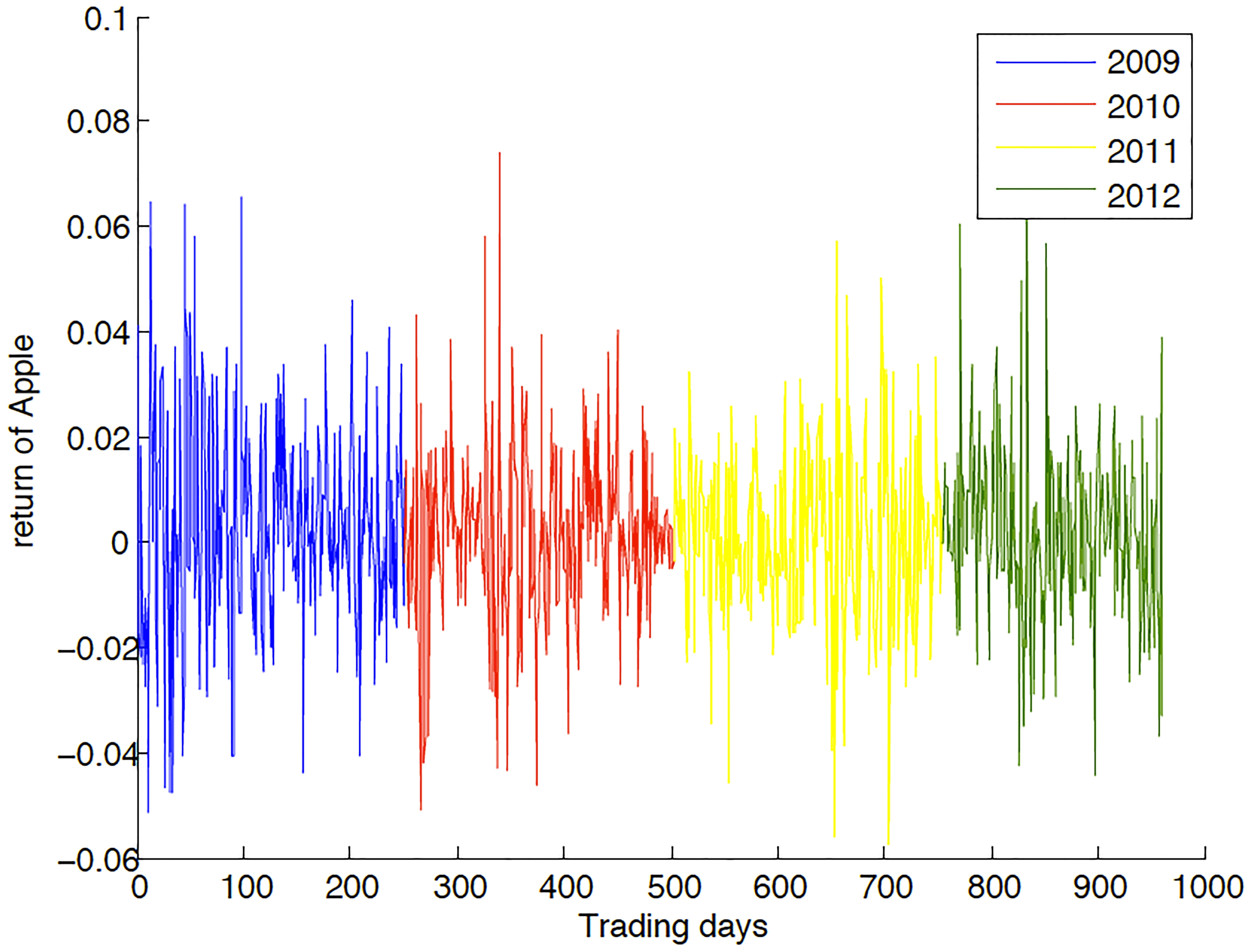
The first data set we use is the discretized in 27 bins daily log-return data of Apple Inc. starting from January 2, 2009.

Figure 2.

Apple log-returns.

By observation, we pick the volatile region (the first 450 days returns) and the quiet region (the 500th to 600th days returns) to make a comparison. We first fit the data with the GARCH(1,1) modeled using the MATLAB(R2011a) GARCH toolbox. The $P$ -values obtained are $P_{1}=$ 0.0311 and $P_{2}=$ 0.0897.

We apply SCOTlr to the same data. The homogeneity $t$ -test between 1–450 and 500–600 (quiet and volatile regions) trained on 1–450 shows that the $t$ -value is $-$ 16.02058. Thus, the $P$ -value $P<$ 0.00001. This $P$ -value by SCOT is dramatically smaller than the $Z$ -score by GARCH.

9. Offline fitting Markov switching model

9.1 HMM model for speech recognition

Speech is modeled (Baum et al) as a sequence of emissions – phonems – random variables $x_{i}$ . Elements of observed sequence $x_{i}$ depend only on current hidden letters of text $z_{i}$ modeled as a Markov Chain. We refer to $z_{i}$ as hidden states, see the Figure above. Inference about the parameters of the model and hidden MC uses only the observed $x_{i},i=1,\ldots$ .

9.2 Slow HMM-SCOT emissions model

We call HMM $z_{i}$ SLOW, if HMM stays mean time proportional to a large parameter $l$ in all states, while the sample size is $kl,k\to\infty$ . Emissions shown in dark in the previous Fig. are modeled as STRINGS of MC over the space of contexts with transition matrix depending on the current HMM state.

Remark. Our HMM-SCOT model has nothing in common with VLMCHMM which analyzes independent emissions under a SCOT model for HMM Dumont (2014).

The emissions MC $x_{i}$ over the alphabet of SCOT contexts are assumed ergodic, different for all states of HMM, expectations are taken under their stationary distributions.

For notation simplicity we start with two-state ( $\pm$ 1) HMM.

Introduce stationary log-likelihoods $l_{i}=\log P(x_{i}|x_{i-1})$ and entropy of SCOT(( $\pm$ 1)): $h$ (( $\pm$ 1)) $=\lim_{M\to\infty}$ $M^{-1}E(\sum_{1}^{M}l_{i})$ .

9.3 HMM-SCOT model fitting

As explained before, the SCOT emissions can be reduced to a MC on the alphabet $\mathcal{B}$ of SCOT contexts.

We assume that diagonal elements of all $Q$ hidden HMM $X_{n}$ transition probability matrices are $a_{i}(l)=(1-(c_{i}l)^{-1})>0,i=1,\ldots,Q,l\to\infty$ and emission distributions are all different. Emission SCOT sequences are assumed transformable to ergodic MC $y_{i},\tau_{j}<i<\tau_{j+1}$ over the same alphabet $\mathcal{B}$ switching from a regime to alternative one at random CP time moments $\tau_{j},j=1,\ldots,Q$ ; $\tau_{0}=$ 0.

We estimate both emission regimes, all CPs and HMM parameters. Thus, the HMM jumps to an alternative state after spending asymptotically exponentially distributed time with mean $c_{i}l$ in each state.

We modify the two settings of Change Point (CP) detection of IID sequences $m_{i}+\mu_{j}$ with changing mean $\mu_{j},j=\pm$ 1 in Korostelev (2011). In their offline method, the quadratic risk of ML as a CP estimate does not exceed $O(1)$ as the sample size $n\to\infty$ due to certain exponential bounds. Their online method uses CP detection which is a point in the first $N$ -interval, $N=O(\log n)$ such that the maximal absolute deviation of $m_{i}$ deviation in this interval becomes comparable with the absolute change of mean $\mu$ .

Our plan for online CP detection is to replace their IID-based inequalities with the Doob-Meyer decomposition-based bounds for the maximal absolute deviation of both the martingale and compensator parts separately. We use the exponential bounds obtained in Section 5.4. By implementing this program, we get the same order of quadratic risk as derived in Korostelev (2011) for IID case with changing mean.

.

A rougher estimates of the quadratic risk in online preliminary CP-detection can be obtained by a simpler quadratic maximum martingale deviation bound guarantying a larger window of order $O(\sqrt{n})$ . It would require much larger risk and sample size, thus it is omitted.

Our algorithm uses repeatedly training (Section 12) the SCOT emissions in all regimes and homogeneity testing of Section 8.1.

To simplify notation, we first present our HMM-MC model with the two-state HMM ( $Q=$ 2).

9.4 Algorithm road map, two-state HMM

For notation simplicity we start with the two-state HMM ( $A=$ 2, $b=\pm$ 1). Our algorithm includes:

1.
Online estimation of the $B\times B$ -transition matrix $P_{-1}$ of 1-MC equivalent to SCOT-emission-regime, see Appendices 1 and 2.
2.
After some initial period of online continuous improving the $P_{-1}$ estimate, start online detection of the first CP $\tau_{1}$ in sequences of windows of size $O(\log l)$ and find a preliminary first CP estimate. We show that its StD is $O(\log l)$ .
3.
The emissions from the time interval exceeding the CP estimate in $(l\varepsilon)^{a}$ , $a>$ 0 are used for online continuous estimation of the alternative regime $P_{1}$ and next CP $\tau_{2}$ .
4.
Using $P_{j},j=0,1$ , estimates we update preliminary CP online estimates with the offline MLE. The offline MLE has StD $=O(1)$ .

Using the approach from the preceding item, we recurrently find estimates of all subsequent CPs and improve estimates of regimes $P_{j},j=\pm$ 1.
5.
Using all CP estimates, we get MLE of the HMM parameters.

9.5 Online CP detection

Given a 1-MC transition matrix in region 1, we carry on the CP online detection between regimes 1 and $-$ 1.

We choose such a window size that within window

$\displaystyle P\left(\max|m(k)|>0.1(\Delta h)\sum c(k)\right)<l^{-3},$ (8)

where $\Delta h$ is the entropy difference between the current and alternative regime. A lower bound for $\Delta h$ is used if $\Delta h$ is unknown. This window size is evaluated using the maximal inequality for absolute value of martingale $|m(\cdot)|$ , Section 4.2. Our CP-detector is the first window when Eq. (5) occurs.

The Borel-Cantelli lemma implies that only finite number of events Eq. (5) occur under $l\to\infty$ . As follows from section , the window size is $O(|\log l|)$ which implies the same order of the standard deviation of our CP detector.

9.6 Offline CP detection

Our offline segmentation stage estimates time regions with constant HMM states using homogeneity test for SCOT emission strings and a preliminary online segmentation. This is made fast recurrently in parallel on a cluster of computers.

The offline CP detection follows after the online CP estimate is obtained. It starts with the SCOT training of the string after small delay of length $O(\log n)$ . The homogeneity test verifies significance of new regime distinction from the previous one. The offline CP update of the preliminary online CP estimate is the location of the maximum of the log-likelihood function.

For simplicity of notation assume that the initial regime is $P_{-1}$ and the time of the first CP is 0. Introduce a surrogate ‘log-likelihood function’ $L_{z}$ under ‘possibly false CP’ at time $z$ and show that $\max L_{z}$ is attained ata point $z_{*}:E(z_{*})^{2}=O(1)$ .

Family $L_{z}=I+\textit{II}+\textit{III}$ is irregular and methods of Section 6 are inapplicable. First suppose $z<$ 0 and $[\pm n]$ is included into exactly two regimes $\pm$ 1; 0 belongs to the online CP interval estimate.

We have

$\displaystyle\textit{I}=\sum_{-n}^{z}l(X(k),X(k-1)),$ $\displaystyle\textit{II}=\sum_{z}^{0}\lambda(X(k),X(k-1)),$ $\displaystyle\textit{III}=\sum_{0}^{n}\lambda(X(k),X(k-1)),$

where $Q_{X(k),X(k-1)},\lambda(X(k),X(k-1))$ are regime $(+1)$ transition probabilities and their logarithm.

Every summand in II has mean $E_{P}\lambda=E_{P}(l)-\delta_{-1}$ . Thus $E_{P}(L_{0}-L_{z})\geqslant z\delta_{-1}$ .

The case $z>$ 0 is dealt with quite similarly resulting in equality $E_{Q}(L_{0}-L_{z})\geqslant z\delta_{+1}$ . Both cross-entropies $\delta_{\pm 1}$ are positive.

The offline interval CP estimate can be updated in many ways including bification for iterative numerical finding $z_{*}$ .

It remains to bound its quadratic risk from above. The lower bound of the same order of magnitude follows from the IID case with changing mean in Korostelev (2011).

Lemma 1 implies that the compensators for $L_{z}$ are maximal at a point $O(1)$ . Convergence of the normalized maximal absolute difference between the compensator and its mean $H_{n}$ to 0 follows from Lemma 1.

The functional CLT for the martingale component of log-likelihood Biscup (2011), Theorem 2.11, states that the normalized martingale sequence converges weakly to the Brownian motion. Our exponential bounds show that the maximal deviation converges to 0 also in $L^{2}$ .

The normalized left log-likelihood over negative times $[-n,0]$ was proved in Section 5.2 to be asymptotically Normal with positive left slope and variance $\sigma_{-}^{2}$ . Similarly, the normalized right log-likelihood of the reverted MC (which is also ergodic) over positive times has negative slope at 0 and variance $\sigma_{+}^{2}$ . Thus, the quadratic risk of $z_{*}$ is $O(1)$ in the weak convergence sense. The mean square convergence can be justified in a standard way.

The SCOT is proved to be LAN which implies that the same orders of quadratic risk remain valid when using the estimated SCOT parameters during search for CP.

9.7 HMM with finite number of states

Training SCOT for the general $m$ states slow HMM model such that all time means spent in states before jump are proportional to large parameter $n$ . Main steps of training are similar to the two HMM state case. Online change point detection is used before every jump to unknown state.

Main steps of training are similar to the two-states HMM case. Online change point detection is used before every jump to unknown state. It is followed by the SCOT training of the string using some delay after jump, where homogeneity is verified by homogeneity test and by the subsequent maximum likelihood offline change point update of the preliminary CP online estimate as above.

After all change points are safely estimated, parameters of HMM are ML-estimated based on their multivariate statistics.

9.8 HMM parameters estimation

If it is only known that all mean times spent in every state before jump are proportional to large parameter $l$ , we can estimate all HMM transition probabilities after detecting all jump times. The marginal HMM distribution is estimated via maximum likelihood applied to the joint CP estimates using obvious frequencies. Namely, denoting $n_{ij}=$ number of times $i$ is followed by $j,j=\pm$ 1, under the stationary initial distribution, the log-likelihood is (see e.g. Billingsley, 1961)

$\displaystyle l(p)=\sum_{ij}n_{ij}\log p_{ij},\sum_{j}p_{ij}\equiv 1,$

which yields the ML estimates

$\displaystyle\hat{p}_{ij}=n_{ij}/\sum_{j}n_{ij}.$

Thus, the average of empirical mean times before estimated jump from $i$ to any $j\neq i$ , serves as an estimate of mean time spent in $i$ , while transition probability from $i$ to any $j\neq i$ is estimated via the last formula or simply as the frequency of jumps from $i$ to $j$ out of all visits to $i$ .

9.9 Confidence band for HMM parameters

The above estimation of the HMM parameters $p_{ij}$ is a regular statistical problem with non-degenerate Fisher Information matrix $I(p)=E_{\pi}\partial l\partial l^{T}/n$ , the offline CP estimates are independent ‘observations’ with square risks of order $O(1)$ not affecting asymptotics of the quadratic risk of ML-estimates. Thus asymptotically,

$\displaystyle\textit{Cov}(\hat{p})=[I(p)n]^{-1}.$

For large state space, iterative methods via Fisher scores are available.

10. Discussion and acknowledgments

Our display of modeling and asymptotic inference of strongly mixing stationary sequences differs drastically from the material presented in traditional courses on stationary processes and connects this discipline with the classical MC-theory. Our AN derivation for ATF, exponential bound for the martingale part of log-likelihood and its application for the online and offline CP detection seem new.

A challenging open problem is to prove accurate asymptotic results for MC alphabet rising simultaneously with the sample size.

Appendix 3 reviews results of Zhang (2017), several revised parts of Malyutov (2012) are used elsewhere in the text including a simulation prepared by Grosu. The author is deeply grateful to them for the long collaboration and help.

Footnotes

Appendix 1: Asymmetric cyclic RW

To illustrate what happens when both $A$ and sample size $N$ grow to infinity, let us consider the asymmetric cyclic random walk (RW).

The alphabet consists of equidistant circumference points $\exp(2ik\pi/A),k=0,1,\ldots,A-1$ , $i$ is the imaginary unit. The asymmetric cyclic random walk stays in the same state and jumps to the nearest left state with probabilities 1/2. Introduce $\theta=\exp(2i\pi/A),s_{r}=((1/2)(1+\theta^{r})$ . Equation (2.11) of Feller (1967) establishes the power $n$ of transition matrix spectral decomposition

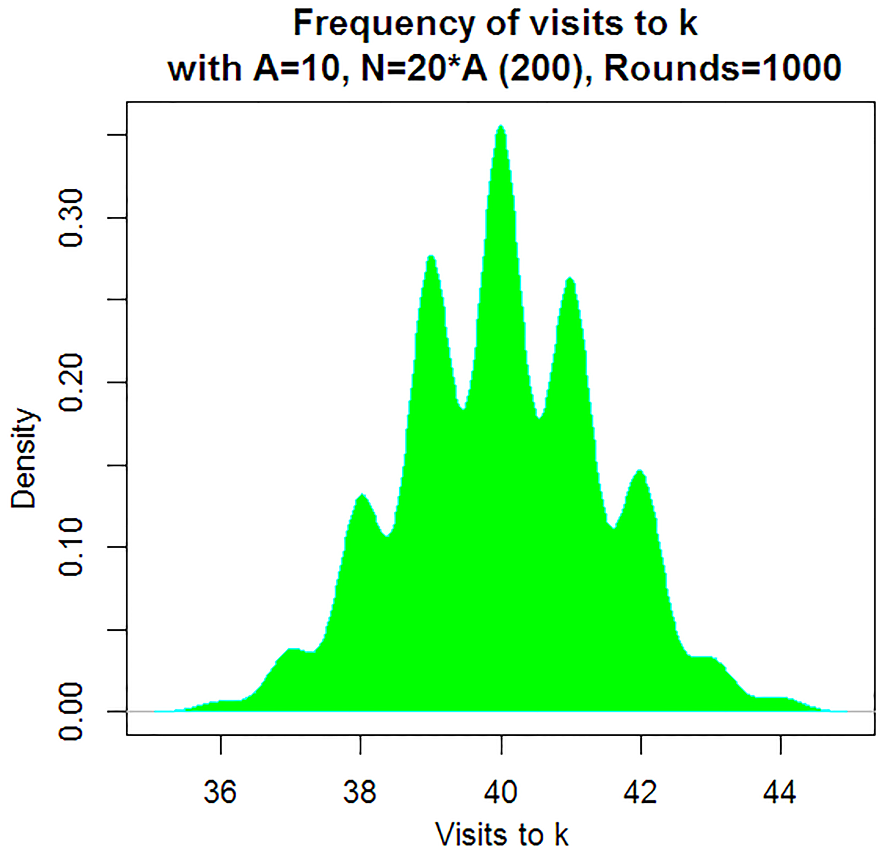
(9) $\displaystyle p_{jk}^{(n)}=(A^{-1})\sum_{r=0}^{A-1}\theta^{r(j-k)}s_{r}^{n}.$

We see from Eq. (1) that eigenvalues of the transition matrix are $O(A^{-1})$ apart as $A\to\infty$ which means that we cannot separate the maximal of them from the rest and restrict spectral expansion to just one ‘maximal summand’. The term $p_{jk=0}^{(A/2)}$ corresponds to the additive state function for the indicator function of state $A/2$ . Obviously, this function takes the value 0, if the initial state is 1 and number of summands less than $A/2$ . Distribution of the sum is far from Normal, if few more summands are involved.

This fact is displayed in empirical histogram of visits to the state $A/2$ (Fig. 1), where the sample size $N$ is 20 times more than $A$ prepared by Grosu as a result of 1000 simulations. It shows several slightly intersected clusters far from the overall Normal histogram.

A similar picture holds for symmetric cyclic RW starting from 0 since it takes at least $A/2$ steps to reach $A/2$ .

Figure 3.

Histogram.

Appendix 2: Parallel SCOT training

This section outlines a novel parallel implementation of the algorithm similar to ‘Context’ which is created for fast processing more complex data sets including those with larger alphabet sizes.

The ESI-based criterion usually stops back-processing of the training string long before the chosen horizon. All directions backwards from the root are processed in parallel making the algorithm much faster. written using the Python programming language – builds the stochastic trees starting from stage 1 and proceeding to the horizon stage of interest. Potential contexts having an ESI value smaller than $\epsilon>$ 0 become contexts, and would be omitted from processing in the following stages. Another improvement in parallelism is processing of a potential context by hashing, and determining if it should be processed on one node of many by taking the modulo of the hash with the total number of compute nodes. The assumption here is that there we have many (hundreds) of compute nodes available to process a corpus into a SCOT.

Appendix 3: Outline of the perfect memory theory,Zhang (2017)

Theory of perfect memory SCOT plays an important role in our constructions. It enables application of abundant theory for 1-MC justifying statistical properties of cumbersome calculations performed by a sophisticated software over SCOT. For completeness, we outline results of Zhang (2017) enabling this reduction.

If each node of a context tree is either a leaf or has exactly $A$ children then it is called complete

For two strings $u,v\in S$ , denote the concatenation of $u$ and $v$ in the natural ordering by $\overline{uv}$ . We say that a string $v\in S$ is a postfix of a string $s\in S$ , denoted by $v\prec s$ , if there exists a string $w\in S$ such that $s=\overline{wv}$ .

For a context tree $\mathcal{T}$ let us denote by $\mathcal{T}_{1},\mathcal{T}_{2},\ldots,\mathcal{T}_{n}$ the sub-trees rooted at the children of $\mathcal{T}$ ’s root. For two context trees $\mathcal{T},\mathcal{T}^{\prime}$ let us write $\mathcal{T}^{\prime}\subseteq\mathcal{T}$ if $\mathcal{T}^{\prime}$ is contained in $\mathcal{T}$ such that they have the same root. The main result is the following.

The statement of the theorem can be reformulated as follows: $\mathcal{T}$ has perfect-memory if and only if $\forall i\in\{1,\ldots,n\}$ , either $\mathcal{T}_{i}=\emptyset$ or $\forall c^{\prime}\in\mathcal{T}^{*},\exists c\in\mathcal{T}_{i}^{*}$ , s.t. $c\prec c^{\prime}$ .

The partially ordered set of perfect-memory context trees is a lattice (namely, intersections and unions preserve perfect-memory), which in turn allows to talk about the perfect-memory closure of a context tree.

Since perfect-memory is closed under intersection, we can define the following.

Perfect-memory is preserved under intersection, so the perfect-memory closure $\overline{\mathcal{T}}$ of a context tree $\mathcal{T}$ has perfect-memory. Thus, $\overline{\mathcal{T}}$ is the minimal context tree that contains $\mathcal{T}$ and has perfect-memory.

Let $C(\mathcal{T})$ denote the minimal complete context tree that contains $\mathcal{T}$ .

An additional goal is to give a simple construction algorithm of the perfect-memory closure of an arbitrary context tree.

Appendix 4: Simulation of CP detection (Feng)

We simulate the first state transfer in HMM $s_{t}$ with states 0 and 1, starting from HMM state 0. The transition probability of this Hidden Markov Model is: $P(s_{1}=0)=$ 1, $P(s_{t}=1|s_{t-1}=0)=$ 0.001, $P(s_{t}=1|s_{t-1}=1)=$ 1, $s_{0}=$ 0. Introduce CP as the least $t$ such that $s_{t}=$ 1.

Then

$\displaystyle P(CP=i)=0.999^{i-1}*0.001\text{ for }i>1.$

In our simulation $s_{t}$ never goes back to state 0 again.

Emissions follow the SCOT model 2.ii from Ryabko (2016); Malyutov (2014).

ii) Define SCOT under state 0: Let

$\displaystyle z_{0}=-1,z_{1}=0$

If $z_{t-1}=-l$ where $-l$ is the left boundary, then:

$\displaystyle z_{t}=-l+1$

If $z_{t-1}=l$ where $l$ is the right boundary (we assume $l$ is large enough such that we will not reach the right boundary in simulation), then:

$\displaystyle z_{t}=l-1$

If for the greatest $k<t$ such that $z_{k}\neq z_{k-1}$ , we have $z_{k}=z_{k-1}+1$ and $z_{t-1}\neq 0$ , then:

$\displaystyle z_{n}=\left\{\begin{array}[]{ll}z_{t-1}+1&\text{with probability% 0.8}\\ z_{t-1}&\text{with probability 0.1}\\ z_{t-1}-1&\text{with probability 0.1}\end{array}\right.$

If for the greatest $k<t$ such that $z_{k}\neq z_{k-1}$ , we have $z_{k}=z_{k-1}-1$ and $z_{t-1}\neq 0$ , then:

$\displaystyle z_{n}=\left\{\begin{array}[]{ll}z_{t-1}-1&\text{with probability% 0.8}\\ z_{t-1}&\text{with probability 0.1}\\ z_{t-1}+1&\text{with probability 0.1}\end{array}\right.$

iii) Under state 1 we use model 2(ii) with probabilities 0.6, 0.2, 0.2 (the previous model is represented by 0.8,0.2,0.2)

Simulating HMM and SCOT models we generate data. Then the CP detection algorithm of Section 7 detects the CP in generated data $z_{1},\ldots,z_{1000}$ . In our simulation displayed in Fig. 1 the sample size is 1000 (i.e. $t=1,\ldots,1000$ ) and the actual single change point is 662.

References

Aminikhanghahi

, & Cook

D.A.

(2017). Survey of methods for time series change point detection. Knowl Inf Syst, 51(2), 339-367.

Billingsley

(1961). Statistical Inference for Markov Chains. University of Chicago Press.

Biscup

(2011). Recent progress on the random conductance model. Probability Surveys, 8, 294-373.

Borovkov

A.A.

(1998). Ergodicity and Stability Of Stochastic Processes. Wiley.

Bradley

R.C.

(2005). Basic properties of strong mixing conditions. A survey and some open questions. Probability Surveys, 2, 107-144.

Brodsky

B.E.

, & Darkhovsky

B.S.

(1993). Nonparametric Methods in Change-Point Problems. Kluwer, Dodrecht.

Chibisov

D.M.

(2009). Lectures on the asymptotic theory of rank tests. Lecture Notes NOTs 14. M: Matematicheskiy Institut im. V. A. Steklova, RAN, In Russian.

Cover

T.M.

, & Thomas

J.A.

(2006). Elements of Information Theory, Second Edition. Wiley, Hoboken.

Cappe

Moulines

, & Rydyen

(2005). Inference in Hidden Markov Models, Springer.

10.

Dumont

(2014). Context tree estimation in variable length hidden markov models. IEEE Trans Inform Theory.

11.

Durbin

Eddy

Krogh

, & Mitchison

(1998). Biological Sequence Analysis. Cambridge University Press.

12.

Feller

(1967). An Introduction to Probability Theory and its Applications, Volume 1, Third edition, Wiley, NY.

13.

Gallager

(2013). Stochastic Processes: Theory for Applications, Cambridge Uni.

14.

Galves, A. & Loecherbach

(2008). Stochastic chains with memory of variable length. Festschrift in Honor of Jorma Rissanen on the Occasion of his 75th Birthday, Tampere, TICSP series No. 38, Tampere Tech Uni, 117-134.

15.

Grinstead

, & Snell

(2006). Introduction to Probability, AMS.

16.

Hamiltons

(2008). Regime switching models. The New Palgrave Dictionary of Economics. Second Edition Durlauf

S.N.

, & Blume

L.E.

, Palgrave Macmillan.

17.

Kharin

, & Maltsau

(2014). Markov chain of conditional order: Properties and statistical analysis. Austrian Journal of Statistics, 4(3-4), 205-216.

18.

Korostelev

, & Korosteleva

(2011). Mathematical Statistics: Asymptotic Minimax Theory, AMS, Providence, RI.

19.

Mächler

, & Bühlmann

(2004). Variable length Markov Chains: Methodology, computing, and software. Journal of Computational and Graphical Statistics, 13(2), 435-455.

20.

Malyutov

, & Protassov

(2002). LAN and LAM, convergence of iterative estimates and optimal design in Gaussian one-way mixed model. Journal of Statistical Planning and Inference, 100(2), 249-279.

21.

Malyutov

, & Grosu

(2017). SCOT approximation, modeling and training. Proceedings of Machine Learning Research, 60, 241-265.

22.

Malyutov

M.B.

Zhang

, & Li

(2013). Time series homogeneity tests via VLMC training. Information Processes, 13(4), 401-414.

23.

Malyutov

M.B.

Zhang

, & Grosu

(2014). SCOT stationary distribution evaluation for some examples. Information Processes, 14(3), 275-283.

24.

Markov

A.A.

(1906). Extension of the limit theorems of probability theory to a sum of variables connected in a chain (in Russian). Appendix B of: Howard R (1971) Dynamic Probabilistic Systems, Volume 1: Markov Chains. John Wiley and Sons.

25.

Malyutov

(2017). Retrospective training slow HMM-SCOT emissions model. Information Processes, 17(3), 199-205.

26.

Meyn

S.P.

, & Tweedy

R.L.

(1993). Markov Chains and Stochastic Stability. Springer.

27.

Rabiner

(1989). A tutorial on hidden Markov models and selected applications in speech recognition. Proceedings of IEEE, 77(2), 257-286.

28.

Rissanen

(1983). A universal data compression system. IEEE Trans Inform Theory, 29(5), 656-664.

29.

Roussas

(1972). Contiguity of Probability Measures: Some Applications in Statistics. Cambridge University Press.

30.

Ryabko

Astola

, & Malyutov

(2016). Compression-Based Methods of Prediction and Statistical Analysis of Time Series: Theory and Appllications. Springer International.

31.

Shiryaev

A.N.

(1978). Optimal stopping rules. Applications of Mathematics, 8, Springer, New York.

32.

Tutubalin

V.N.

(1992). Probability and Random Processes Theory. Mathematical Foundations and Applications. Moscow State University Press (In Russian).

33.

Veretennikov

A.Yu.

(2000). Parametric and Nonparametric Estimation for Markov Chains. Moscow State University Press (In Russian).

34.

Veretennikov

A.Yu.

(2017). Ergodic Markov Chains and Poisson equations (lecture notes). Arxiv:1610.09661v3 [math PR].

35.

Volkonskii

V.A.

, & Rozanov

Yu.A.

(1959). Some limit theorems for random functions I. Theor Probab Appl, 4, 178-197.

36.

Yoon

B.J.

(2009). Hidden Markov models and their applications in biological sequence analysis. Current Genomics, 10(9), 402-415.

37.

Zhang

(2017). Perfect memory context trees in time series modeling. Information Processes, 17(1), 70-81.