Continuous time nonstationary correlation models for sparse longitudinal data

Abstract

In this paper, we present a new continuous time model for nonstationary correlation structures for longitudinal data. This model, which provides a continuous time analogue to the antedependence model and is thus referred to as the continuous antedependence (CAD) model, is intended to provide more refined correlation models for longitudinal data and to better accommodate sparse (or highly unbalanced) data. A key component of this model is the ‘nonstationarity function’ which describes nonstationarity as a unidimensional function of time and has an interesting time expansion/contraction interpretation. Focusing on a Markovian version of the model, we develop a novel nonlinear regression model providing nonlinear least square estimators of model parameters. Both unstructured (for nonparametric estimation) and structured versions of the model are presented. We apply the proposed approach to data from the Multicenter AIDS Clinical Study (MACS), with a focus on inference for the nonstationarity function. In simulation studies, we show good properties (low finite sample bias, and high convergence rates and efficiency) of the proposed unstructured model estimator, which compare favorably to those of an alternative maximum likelihood estimator, particularly in sparse data situations.

Keywords

Antedependence covariance structures Markovian maximum likelihood estimation missing data nonlinear least squares repeated measures

1. Introduction

The analysis of longitudinal, or repeated measures, data often gives much attention to the modeling of the within-subject correlation structure. This task is important for valid and efficient inference for mean structure parameters, as well as for its own scientific interest. Knowledge about the correlation structure can provide insights into the disease/health process. Furthermore, information about correlations is important for future study design. Numerous correlation models have been proposed, some of which, such as the first-order autoregression model (AR(1)), have had wide use and implementation in standard statistical software packages. A ‘spatial’ version of AR(1) (SAR(1)), which involves the actual measurement times rather than just the time index, is useful when measurements are unequally spaced or are at irregular times across subjects.

Many commonly used models, including AR(1) and SAR(1), have the property of stationarity. Stationarity, in the present context, implies that the correlations depend only the time gap between measurements, and not further on the measurement times. Unfortunately, actual biological data seldom follow simple stationary models. In light of this reality, nonstationary models have also been proposed for longitudinal data. One such model that has become increasingly popular is the antedependence model (Gabriel, 1961, 1962; Zimmerman & Núñez-Antón, 2009). Antedependence, like autoregression, can be of varying dependence order with a low (first or second) order antedependence structure often found to be adequate for fitting repeated measures data. A more parsimonious special case of the antedependence model, referred to as the structured antedependence (SAD) model has also been proposed (Zimmerman & Núñez-Antón, 1997; Núñez-Antón & Zimmerman 2000).

A further challenge in many longitudinal studies is the presence of sparse data, that is, data for which the number of measurement times is large relative to the total number of measurements, so that very few measurements may be available at each time point. Maximum likelihood estimation algorithms, while typically accommodating missing data (usually making a missing at random assumption (Rubin, 1976)), often have convergence problems with very sparse data.

This paper presents a new continuous time version of the first-order antedependence model, which we refer to as the continuous antedependence model (CAD). This new model is particularly suited to handling sparse longitudinal data, as may be expected from observational designs or even randomized studies with irregular measurement times. The proposed model features a newly defined nonstationarity function which we highlight as an object of interest in its own right. Further, a novel nonlinear least squares (NLLS) approach to parameter estimation for the CAD model is presented. We illustrate the new approach with an application to data from an AIDS observational study and demonstrate favorable properties of the proposed estimators in a simulation study. We conclude with a discussion of limitations and some future directions.

2. Background: Discrete antedependence

The classical formulation of antedependence (Gabriel, 1961, 1962) states that a sequence of random variables, $Y_{1},Y_{2},\ldots,Y_{m}$ , has an antedependence structure of order $s$ if $Y_{j}$ and $Y_{j+k+1}$ are independent given $Y_{j+1},Y_{j+2},\ldots,Y_{j+k}$ , for $j=1,2,\ldots,m-k-1$ and for all $k\geqslant s$ , $s=0,1,\ldots,m-1$ . Typically, the index $j$ ( $j=1,\ldots,m$ ) refers to a time order with corresponding fixed times, $t_{1}<t_{2}<\ldots<t_{m}$ . The 0th order model is equivalent to independence among the $m$ responses, while the ( $m-1$ )th order case corresponds to an unstructured covariance matrix. A parametric version of this model (Gabriel, 1962; Núñez-Antón & Zimmerman, 2000), equivalent to the above definition when $\bm{Y}\equiv(Y_{1},\ldots,Y_{m})^{\prime}$ is $m$ -variable normally distributed, can be written as, $Y_{1}=\mu_{1}+\varepsilon_{1}$ , $Y_{j}=\mu_{j}+\sum_{k=1}^{s_{j}}\rho_{j-k,j}(Y_{j-k}-\mu_{j-k})+\varepsilon_{j}$ , $j=2,\ldots,m$ , where $s_{j}=\min(s,j-1)$ ; $\bm{\mu}\equiv(\mu_{1},\ldots,\mu_{m})^{\prime}$ is the mean vector of $\bm{Y}$ ; the $\varepsilon_{j}$ ’s are independent unobserved error terms with zero means and variances $\sigma_{j}^{2}>$ 0; and the $\rho_{jk}$ ’s (with $\rho_{jk}$ representing the correlation between $Y_{j}$ and $Y_{k}$ ) are such that the covariance matrix of $Y$ is positive definite. The resulting covariance model will be referred to as AD( $s$ ). The first-order AD model, AD(1), satisfies the multiplicity property, $\rho_{jl}=\rho_{jk}\rho_{kl}$ , equivalently, $\rho_{jl}=\prod_{i=j}^{l-1}\rho_{i,i+1}$ , for all $j<k<l$ , and the covariance for measurements at the $j$ th and $l$ th time points is $\sigma_{jl}=\sigma_{j}^{2}\sigma_{l}^{2}\prod_{k=j}^{l-1}\rho_{k,k+1}$ . In this first-order case, we write for brevity, $\rho_{j}\equiv\rho_{j,j+1},j=1,\ldots,m-1$ .

Inference for the AD model was discussed by Gabriel (1962) and further studied by Byrne and Arnold (1983), Albert (1992), Macchiavelli and Arnold (1994), Macchiavelli and Moser (1997), Zimmerman and Núñez-Antón (1997), Núñez-Antón (1998), Zimmerman et al. (1998), Al-Ibrahim (1999), Krzanowski (1999), Núñez-Antón and Zimmerman (2000), and Zhang (2005). Typically, multivariate normality is assumed for $\bm{Y}$ and maximum likelihood methods used for inference. In the case of a common set of measurement times for the $n$ subjects, and a common AD covariance matrix, $\bm{\Sigma}$ , an explicit expression can be written for the maximum likelihood estimator of $\bm{\Sigma}$ (see Byrne & Arnold 1983; Albert 1992).

In the common situation in which subjects have missing data, let $\bm{\Sigma}_{i}$ denote the $m_{i}\times m_{i}$ covariance matrix (a submatrix of the $m\times m$ complete data covariance matrix, $\bm{\Sigma}$ ) for individual $i$ with $m_{i}$ measurements. In the case of missing data, explicit estimators generally are not available, and numerical methods must be used to maximize the likelihood (or restricted likelihood) function. Zimmerman et al. (1998) further discussed computational issues for maximum likelihood estimation for the AD(1) model in the context of missing data (an issue also addressed earlier by Patel (1991)). In particular, they suggested an approach to reduce computation by using simplified expressions for elements of the inverse of the AD(1) covariance matrix. More general algorithms are also available; for example the MIXED procedure in SAS implements Newton Raphson algorithms for fitting the general linear model with flexible covariance structures, including AD(1), while also allowing for general patterns of missing data, including both monotone (dropouts) and non-monotone (or intermittent) missingness.

A structured version of AD(1), proposed by Zimmerman and Núñez-Antón (1997) is given by

$\displaystyle\rho_{j}=\rho^{f(t_{j+1};\bm{\lambda})-f(t_{j};\bm{\lambda})},% \quad\sigma_{j}^{2}=\sigma^{2}g(t_{j};\psi)$ (1)

for $j=1,\ldots,m$ , where 0 $<\rho<$ 1, $\sigma^{2}>$ 0, $\lambda$ and $\psi$ are parameter vectors (typically of low dimension), and $f$ and $g$ are known functions. A single-parameter version (given by Zimmerman and Núñez-Antón (1997), and applied earlier by Núñez-Antón and Woodworth (1994)) uses the function $f(t;\lambda)=(t^{\lambda}-1)/\lambda$ if $\lambda\neq$ 0; otherwise, $f(t;\lambda)=\log(t)$ , with 0 $\leqslant\lambda<\infty$ . This special case of the SAD model thus uses the Box-Cox family of power transformations to specify $f(t;\lambda$ ). In this family of models, $\lambda>$ 1 ( $\lambda<$ 1) provide correlations that are increasing (decreasing) with time for a given time gap. For example, repeated responses may be subject to participant ‘learning’ (as was hypothesized in the cochlear implant study analyzed by Núñez-Antón and Woodworth (1994)) thus leading to higher correlations for responses equidistant in time as the study progresses. Note that the SAR(1) model (a stationary model), is obtained as a special case with $\lambda=$ 1.

Although formulated as a reduction of the AD model, and thus based on a fixed set of time points, the SAD model would appear to be applicable to the continuous time case. However, a limitation of this model for continuous time is that it does not provide a function that describes the nonstationarity over continuous time, as the function $f$ does not play this role. Note that the correlations themselves cannot be written as a single-dimensional function of time, or of the time gap as in the stationary case.

3. Proposed method: Continuous time antedependence

3.1 Model

This section introduces the proposed continuous version of the first-order antedependence model, considering the response variable to follow an underlying continuous process. Specifically, $Y^{C}$ , denoting the response variable function, will represent a stochastic process; that is, $Y^{C}=[Y_{t}:t\in[0,T]]$ , a collection of random variables on a probability space ( $\Omega$ , $\mathcal{F}$ , $P$ ). The stochastic process $Y^{C}$ is assumed to have mean function $\mu$ , and variance function $\sigma^{2}$ (both over [0, $T$ ]); its distribution is not further specified.

The proposed model, referred to as the Markovian continuous antedependence (MCAD) model, then describes the correlation between values of $Y^{C}$ at any two time points in the specified range, say $t_{j}$ , $t_{k}$ , 0 $\leqslant t_{j}<t_{k}\leqslant T$ , as

$\displaystyle\phi(t_{j},t_{k})=\rho^{\int_{t_{j}}^{t_{k}}W(t)dt}$ (2)

where $W(t)$ is a specified positive and integrable function for $t\in[0,T]$ . Note that $W(t)$ together with $\rho$ can only be identified within a constant of proportionality, so that some further constraint on $W(t)$ (for example, $W(0)=$ 1) is necessary. The relatively simpler problem of estimation of the variance function (as given in Eq. (1)) is left aside to maintain focus on the correlation structure. A key goal is the estimation of the function $W(t)$ , referred to as the nonstationarity function.

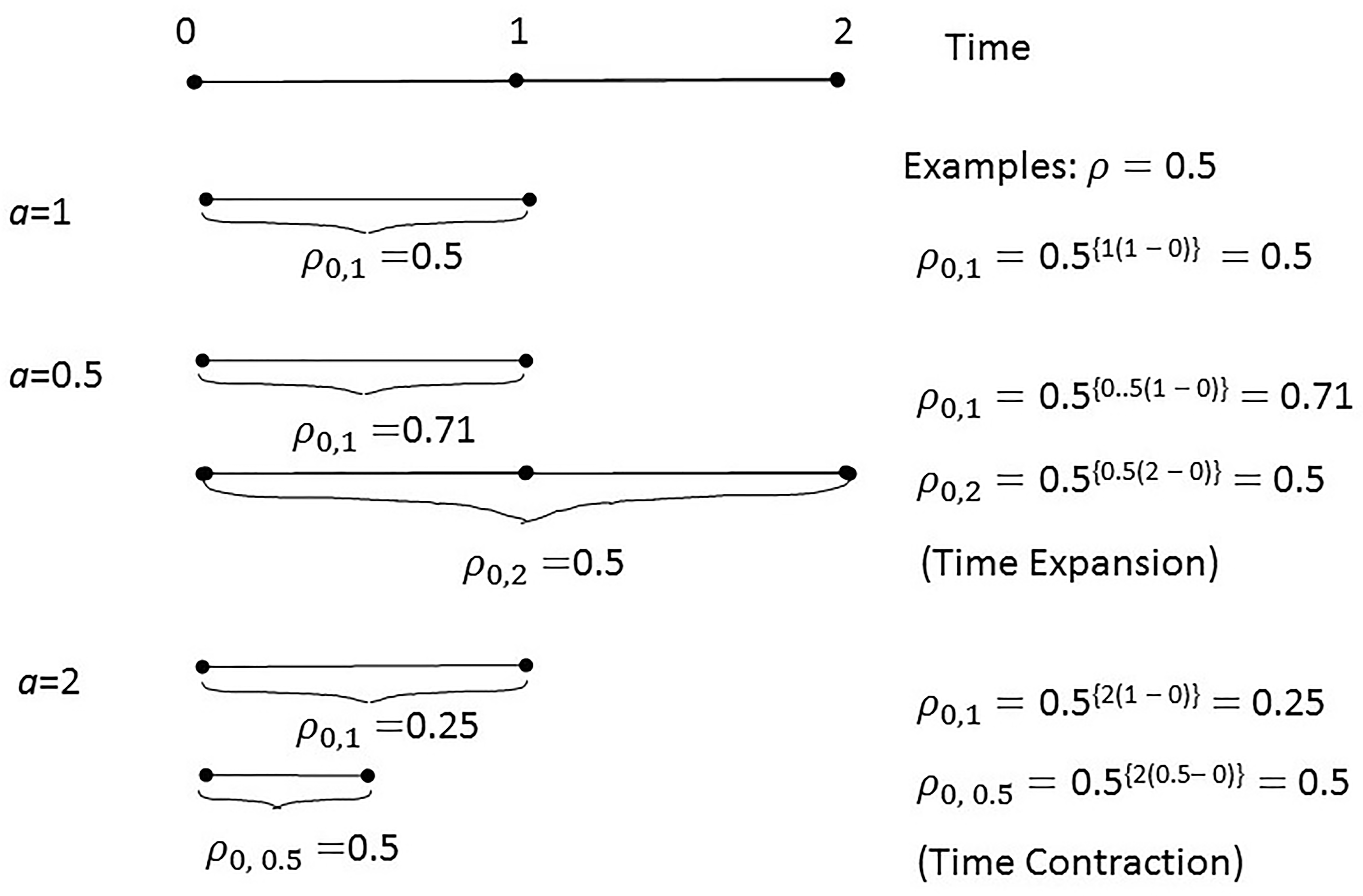
One implication of the MCAD model is that for any (possibly arbitrarily small) interval $[t,t+\Delta]\subset[0,T]$ , within which $W(t)$ is constant, say $W(t)=a$ , the correlations for any two measurements, say $Y_{j}$ and $Y_{k}$ , measured at times $t_{j},t_{k}\in[t,t+\Delta]$ with $t_{j}<t_{k}$ , is given by $\rho^{a(t_{k}-t_{j})}$ . This means that within an interval for which $W(t)=a$ , time is essentially expanded (for $a<$ 1) or contracted (for $a>$ 1) by the factor $a$ relative to a reference interval with $W(t)=$ 1. In other words, measurements that are one unit of time apart in an interval with $W(t)=$ 1 have the same correlation as measurements $1/a$ time units apart in an interval in which $W(t)=a$ . Thus, smaller $a$ implies a higher correlation (and ‘expanded’ time) for a given time interval, while larger $a$ implies a lower correlation (and ‘contracted’ time). This concept is illustrated in Fig. 1 with a numerical example. More generally, $W(t)$ describes the change in local correlations over time. Note that in the special case where $W(t)=$ 1 (or any constant) over [0, $T$ ], implying stationarity, the continuous-time analogue of the first-order autoregressive model (essentially, SAR(1) defined over [0, $T$ ]) is obtained. A second implication of the MCAD model, as implied by the name, is that the response variable, $Y$ , has the Markov property, whereby correlations satisfy the multiplicative property; that is, for ordered times $0\leqslant t_{j}<t_{k}<t_{l}\leqslant T$ , we have $\phi(t_{j},t_{l})=\phi(t_{j},t_{k})\phi(t_{k},t_{l})$ . It follows that the correlation can more generally be written as a product of correlations corresponding to any partition of the interval $[t_{j},t_{l}]$ .

Figure 1.

Time expansion/contraction in the CAD model.

A structured MCAD (SMCAD) model is obtained from Eq. (2) by considering $W(t)$ as a parametric function, written as $W(t;\bm{\lambda})$ . The function, $W(t;\lambda)=t^{\lambda-1}$ , for example, provides a continuous version of the (first-order) SAD model Eq. (1). The connection between the SMCAD and the SAD, where the latter is considered as a continuous model with an arbitrary differentiable function $f(t)$ , is given more generally by the relationship, $W(t)=\frac{df(t)}{dt}$ . If $f(t)$ is non-differentiable at some points (for example, has discontinuities), $W(t)$ may still be defined (e.g., as a step-function). A related note is that, in contrast to previous models, the form of model Eq. (2) essentially unifies unstructured and structured antedependence models.

3.2 Inference

3.2.1 Setup

Suppose a random sample is taken from a stochastic process $\xi$ (with mean function equal to 0 and variance function $\sigma^{2}$ ) satisfying the MCAD model Eq. (2), providing independent random functions $Y_{1}^{C},\ldots,Y_{n}^{C}$ , where $Y_{i}^{C}=\mu_{i}+\xi_{i}$ , $\mu_{i}$ is the fixed mean function and $\xi_{i}$ is the realization of $\xi$ (interpretable as an error function) for individual $i$ . The (latent) random function $Y_{i}^{C}$ is interpreted as the underlying response function for subject $i$ , values of which are observed at a finite (usually relatively small) number of times, possibly arbitrarily chosen, in the range [0, $T$ ]. The observed data thus consist of a response vector $\bm{Y_{i}}=(Y_{i1},\ldots,Y_{im_{i}})$ with measurements at times $t_{i1},\ldots,t_{im_{i}}$ for subject $i,i=1,\ldots,n$ . A common correlation structure for all subjects is assumed, and thus the subscript $i$ will be dropped when not needed for clarity.

In addition, let $r_{ij}$ denote the residual (given a fitted regression model) for the $i$ th subject at this subject’s $j$ th measurement time (namely, $t_{ij}$ ); specifically, $r_{ij}=(Y_{ij}-\hat{\mu}_{ij})/\hat{\sigma}_{ij}$ where $\hat{\mu}_{ij}$ is a suitable estimate of the mean, $\mu_{ij}\equiv\mu_{i}(t_{ij})$ , and $\hat{\sigma}_{ij}$ is an estimate of the square root of the variance, $\sigma_{ij}^{2}\equiv\sigma^{2}(t_{ij})$ . The outcome variable, providing information about the correlation between the successive measurements, may be defined as $R_{ij}\equiv r_{ij}\cdot r_{i,j+1}$ , for $j=1,\ldots,m_{i}-1$ . Note that if $\hat{\mu}_{ij}$ and $\hat{\sigma}_{j}$ are equal to the corresponding population values, then, by definition, $E(R_{ij})=\phi(t_{ij},t_{i,j+1})$ ; that is, the expected value of the outcome is equal to the corresponding population correlation. If $\hat{\mu}_{ij}$ and $\hat{\sigma}_{j}$ are consistent estimates of $\mu_{ij}$ and $\sigma_{j}^{2}$ , respectively, then, $R_{ij}$ is asymptotically unbiased for $\phi(t_{j},t_{k})$ . An alternative construction for the outcome is $R_{ij}\equiv 1-\{0.5(r_{i,j+1}-r_{ij})^{2}\}$ , $j=1,\ldots,m_{i}-1$ . Here, $R_{ij}$ may be seen as a single-observation version of the sample variogram, which is widely used for exploring stationary correlation structures (Diggle et al., 2002).

3.2.2 Nonparametric estimation for the MCAD

A nonparametric approach to inference for the MCAD, providing a step-function estimator of $W(t)$ , will next be presented. Let $\bm{t}\equiv(t_{1},t_{2},\ldots,t_{Q})$ denote the ordered vector containing the distinct measurement times over the whole sample, and let $\rho_{k}$ denote the correlation between measurements (possibly latent for any given subject) at times $t_{k}$ and $t_{k+1}$ for $k=1,\ldots,Q-1$ . Though dependent on the possibly random or arbitrary measurement times, these quantities will be referred to as ‘parameters’ for convenience; the implied correlation model will be referred to as the unstructured MCAD (UMCAD) model.

A regression approach is motivated by considering a pair of adjacent measurements $Y_{ij}$ and $Y_{i,j+1}$ measured at times $t_{ij}$ and $t_{i,j+1}$ for subject $i$ , corresponding, without loss of generality, to (whole sample) times $t_{k}$ and $t_{k+d}$ , for positive integers $k$ and $d$ such that $k<Q$ and $d\leqslant Q-k$ . This pair of measurements provides information regarding $\rho_{k,k+d}\equiv\phi(t_{k},t_{k+d})$ , which will be referred to a ‘gap correlation’. Due to the multiplicative property, this correlation can be written as the following function of the UMCAD correlation parameters:

$\displaystyle\rho_{k,k+d}=\prod_{j=k}^{k+d-1}\rho_{j}=\exp\left\{\sum_{j=k}^{k% +d-1}\log(\rho_{j})\right\}.$ (3)

The identity Eq. (3), and the fact that it holds, at least approximately, after substituting $E(R_{ij})$ for $\rho_{k,k+d}$ , suggest a regression relationship that can be applied to the observed variates, $R_{ij}$ , $i=1,\ldots,n$ , $j=1,\ldots,m_{i}-1$ (defined in the preceding section). Specifically, consider the nonlinear regression model,

$\displaystyle\bm{R}_{i}=\exp(\bm{Z}_{i}\bm{\psi})+\bm{\varepsilon}_{i}$ (4)

where $\bm{R}_{i}\equiv(R_{i1},\ldots,R_{im_{i}-1})^{\prime}$ is the $(m_{i}-1)\times 1$ vector of constructed response variables for subject $i$ , $\bm{Z}_{i}\equiv(\bm{Z}_{i1},\ldots,\bm{Z}_{i,m_{i}-1})^{\prime}$ is the $(m_{i}-1)\times(Q-1)$ design matrix with $\bm{Z}_{ij}\equiv(Z_{ij1},\ldots,Z_{ij,Q-1})^{\prime}$ , $Z_{ijq}=I(t_{i,j}\leqslant t_{q})\cdot I(t_{i,j+1}\geqslant t_{q+1})$ , $\bm{\psi}\equiv(\psi_{1},\ldots,\psi_{Q-1})^{\prime}$ , $\psi_{k}=\log(\rho_{k})$ , $\bm{\varepsilon}_{\bm{i}}$ is an $(m_{i}-1)\times 1$ vector of error terms, and let $\exp(\bm{A})$ denote the matrix with ( $i, j$ ) element equal to $\exp(A_{ij})$ , where $A_{ij}$ is the ( $i, j$ ) element of $\bm{A}$ . It is assumed that $E(\bm{\varepsilon}_{i})=\bm{0}$ , and that the $\bm{\varepsilon}_{\bm{i}}$ are independent, for $i=1,\ldots,n$ . It is further assumed that the $\rho_{k}$ ’s are positive, and since they are bounded by 1, the $\psi_{k}$ ’s are constrained to be negative.

The $\psi_{k}$ ’s in model Eq. (4) may be estimated by minimizing the nonlinear least squares (NLLS) criterion

$\displaystyle S(\bm{\psi})=\sum_{i=1}^{n}\sum_{j=1}^{m_{i}}\left\{R_{ij}-\exp(% \bm{Z_{ij}\psi})\right\}^{2}$ (5)

under the constraints, $\psi_{k}<$ 0, $k=1,\ldots,Q-1$ . The particular numerical approach to this estimation used in this paper is the Levenberg-Marquardt algorithm provided in the SAS subroutine NLPLM and in the SAS NLP Procedure. The resulting regression (log-transformed correlation) parameter estimates are exponentiated to obtain estimates of the UMCAD correlation parameters. Standard errors of the regression parameter estimates are obtained by using the SAS NLPFDD subroutine or SAS PROC NLP; the delta method is then employed to obtain approximate standard errors of the estimated correlations. PROC NLP also provides Wald confidence intervals.

For $W(t)$ considered as a step function, let $a_{k}$ denote the constant value for $W(t)$ in the time interval $[t_{k},t_{k+1})$ , $k=1,\ldots,Q-1$ (setting $a_{1}=$ 1 for identifiability). From the MCAD model Eq. (2) it follows that $\rho_{1}=\rho^{(t_{1}-t_{0})}$ and $\rho=\rho_{1}^{1/(t_{1}-t_{0})}$ . Then, it is easy to show that $a_{k}=\{(t_{2}-t_{1})/(t_{k+1}-t_{k})\}\{\ln(\rho_{k})/\ln(\rho_{1})\}$ , for $k=2,\ldots,Q-1$ . By plugging in the NLLS estimates of the $\rho_{k}$ ’s into the latter expression, estimates of the $a_{k}$ ’s, and thus of $W(t)$ , are obtained. The resulting estimated function is denoted as $\tilde{W}(t)$ .

It is possible with rounded measurement times that there may be replicates (multiple measurements for an individual) at a given putative time. This situation can be handled in the above approach by allowing replicates to provide multiple $R_{ij}$ ’s at some pairs of adjacent times. For example, if a subject has three distinct measurement times with two replicates at his second time point, and one each at his first and third time point, then four (rather than two) $R_{ij}$ ’s will be created, as each replicate provides an $R_{ij}$ with each of its neighboring measurements.

Finally, note that the ‘unweighted’ estimation approach described above assumes that the $R_{ij}$ ’s are independent within individuals. In reality, given the manner of construction of the $R_{ij}$ ’s (using adjacent residuals), this assumption is unlikely to hold exactly (even in the absence of replicates as discussed above). A generalized least squares approach based on derived expressions for the correlations among the $R_{ij}$ (defined as products) is possible. However, the focus of this paper is on the unweighted estimator, an approach that will be justified through the results of a simulation study presented below.

3.2.3 Confidence bands for

W(t)

To do inference regarding $W(t)$ in the MCAD model, a method of obtaining confidence bands for $W(t)$ will be of interest. Our goals for such confidence bands, are: 1) the bounds are nonparametric, and 2) the true $W(t)$ would be entirely contained in ( $1-\alpha$ )% of the confidence bands (obtained under repeated sampling) for selected type I error level $\alpha$ . These characteristics would allow the bounds to be used to test for nonstationarity; specifically, it may be concluded that there is some nonstationarity if the constant function $W(t)=$ 1 (representing the null hypothesis of stationarity when $W(0)$ is fixed at 1) is not fully contained within the bounds.

A bootstrap sampling approach is proposed in which $\tilde{W}(t)$ , the nonparametric estimate of $W(t)$ , is recomputed for each of $N$ (a pre-selected large number of) bootstrap samples. Each bootstrap sample (of the same size as the original data set) is obtained by drawing individuals with replacement. The values of $\tilde{W}(t)$ for all the samples are then ranked at each point in $\bm{t}$ . Let $\tilde{W}_{p}(t_{j})$ denote the rank- $p$ value of $\tilde{W}(t)$ from the bootstrap samples at time $t_{j}$ , and let $\tilde{W}_{p}(t)$ represent the step function connecting the values for $\tilde{W}_{p}(t_{j})$ over all the $t_{j}$ (in order) in $\bm{t}$ . Then the ranks $p=\textit{pmin}$ and $p=\textit{pmax}$ are found such that no more than $(\alpha/2)N$ of the bootstrap estimates of $\tilde{W}(t)$ are lower (higher) than $\tilde{W}_{\textit{pmin}}(t)$ ( $\tilde{W}_{\textit{pmax}}(t)$ ) at any $t_{j}\in[0,T]$ for ‘symmetric’ 100( $1-\alpha$ )% level confidence bands. This procedure assures that the confidence bands contain at least at least 100( $1-\alpha$ )% of the $\tilde{W}(t)$ ’s from the $N$ bootstrap samples. If even the extreme ranks ( $p=$ 1 and $p=N$ ) do not satisfy the above criteria for a given $\alpha$ , then one may need to settle for a larger $\alpha$ level; alternatively, asymmetric confidence bands may be considered. Although this approach satisfies the present objectives, it is possible that a modified approach (e.g, using values of the bootstrap $\tilde{W}(t)$ ’s from varying ranks over the time points) would be more efficient (that is, provide overall narrower confidence regions).

3.2.4 Structured MCAD (SMCAD) model estimation

To do estimation for a SMCAD model, the same setup as described above for the MCAD model can be used. For the SMCAD, we suppose the specification of some structured nonstationarity function $W(t;\bm{\lambda})$ , with $\bm{\lambda}$ denoting a (usually low-dimensional) parameter vector. The nonlinear least squares criterion Eq. (5) can then be modified as,

$\displaystyle S(\bm{\lambda})=\sum_{i=1}^{n}\sum_{j=1}^{m_{i}}\left(R_{ij}-% \phi(t_{j},t_{k};\bm{\lambda})\right)^{2}$ (6)

where $\phi$ represents a parametric correlation function (with parameters given by $\bm{\lambda}$ ); namely, it is a structured version of the MCAD written in terms of the structured nonstationarity function as

$\displaystyle\phi(t_{j},t_{k};\bm{\lambda})\equiv\rho^{\int_{t_{j}}^{t_{k}}W(t% ;\bm{\lambda})dt}.$

Similarly to the approach for the MCAD, an appropriate optimization algorithm (e.g., Levenberg-Marquardt) can be used to estimate $\bm{\lambda}$ , and the delta method may be used to obtain approximate standard errors and confidence intervals. The estimate of $W(t;\bm{\lambda})$ is then obtained by plugging in the estimate for $\bm{\lambda}$ .

4. Data example

In this section, the proposed method is applied to data obtained from the Multicenter AIDS Cohort Study (MACS) public data set (US Department of Commerce, release P16, October 29, 2007). MACS (Kaslow et al., 1987) is an ongoing prospective study of natural and treated histories of HIV-1 infection in homosexual and bisexual men conducted at multiple sites in the U.S. The original cohort, which began in 1984, consisted of 4,954 subjects, while an additional cohort was recruited between 1987 and 1991. The combined cohort was assessed at semiannual follow-up visits for HIV infection status, behavioral outcomes (obtained from questionnaires), and serum levels of a panel of biomarkers.

An important biomarker, considered to be highly predictive of the progression from seroconversion to AIDS, is the CD4+ T-cell count (or CD4 count, for short). A research question of longstanding interest is regarding the pattern of change in CD4 counts over time from seroconversion. Numerous methodological papers have been concerned with the change in mean CD4 over time (Boscardin et al., 1998; Jacqmin-Gadda et al., 2002; Struthers & McLeish, 2011). However, the change in within-person correlations in CD4 over time, which has received less attention, is also of interest (Diggle & Verbyla, 1998; Taylor & Law, 1998). Knowledge of such correlation patterns, particularly considering possible nonstationarity, could shed light on dynamics of AIDS, and help in the design of future studies by indicating times at which measurements would be most informative.

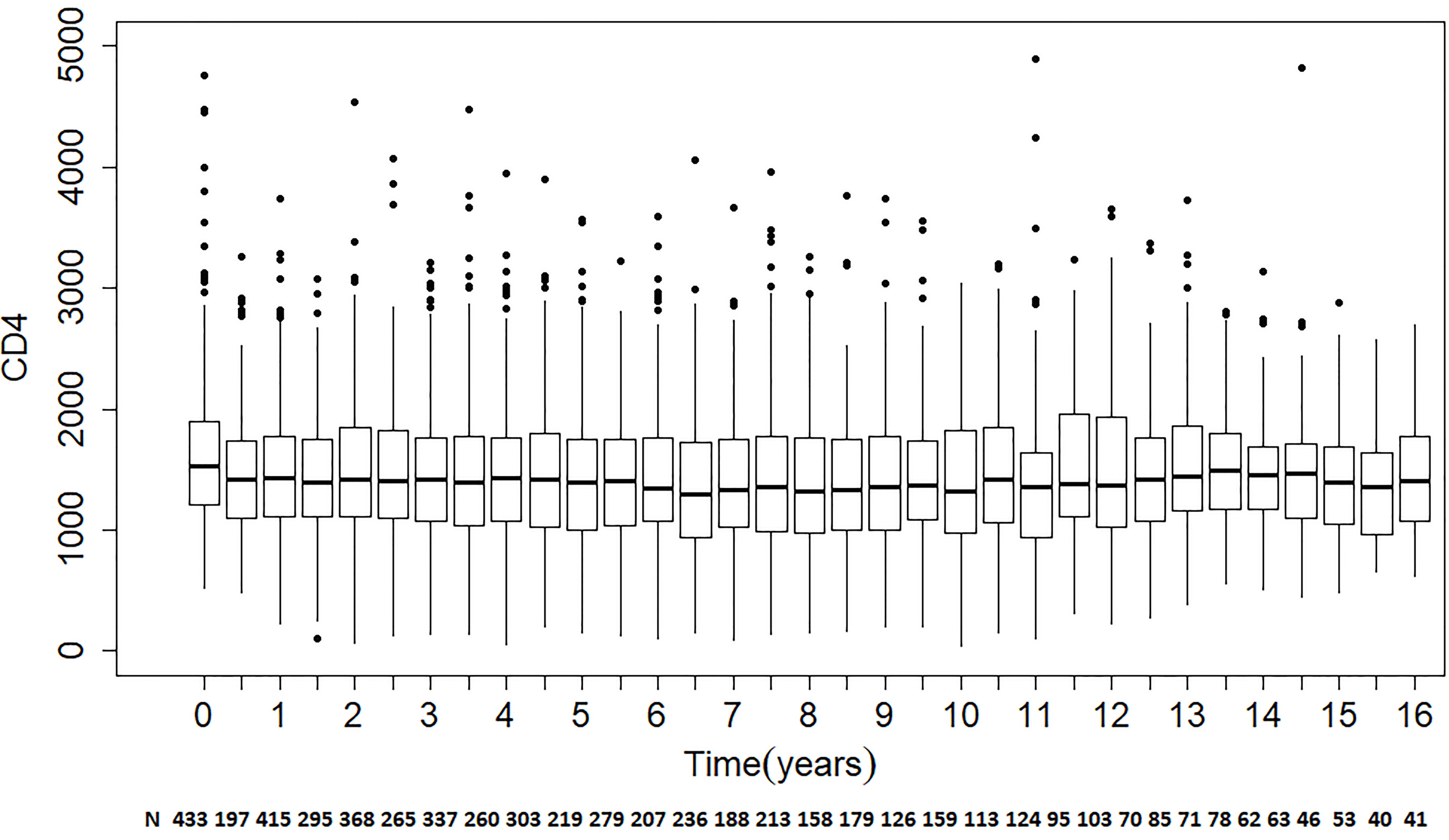
The present analysis used data from 1984 through 1999, including 433 seroconverters. The median follow-up time for this group was five years with a minimum of six months and a maximum of 19 years. For practicality, while retaining relevance to the scientific question of interest, attention was restricted to a follow-up of 16 years, and the data slightly coarsened by taking the time for each measurement to be the closest six-month time point to the recorded date. The median number of CD4 count measurements for the included subjects was 12, with a minimum of one measurement and a maximum of 34 measurements. The number of distinct times over the whole sample for the coarsened data was 33. Note that some subject had ‘replicates’, that is, more than one measurement at the same nominal time point (as is obviously the case for the subject who had 34 measurements). Figure 2 provides box plots of the CD4 counts at each time, revealing sparseness of the resulting longitudinal data.

Figure 2.

Box plots of CD4 counts over time for MACS data

Figure 3.

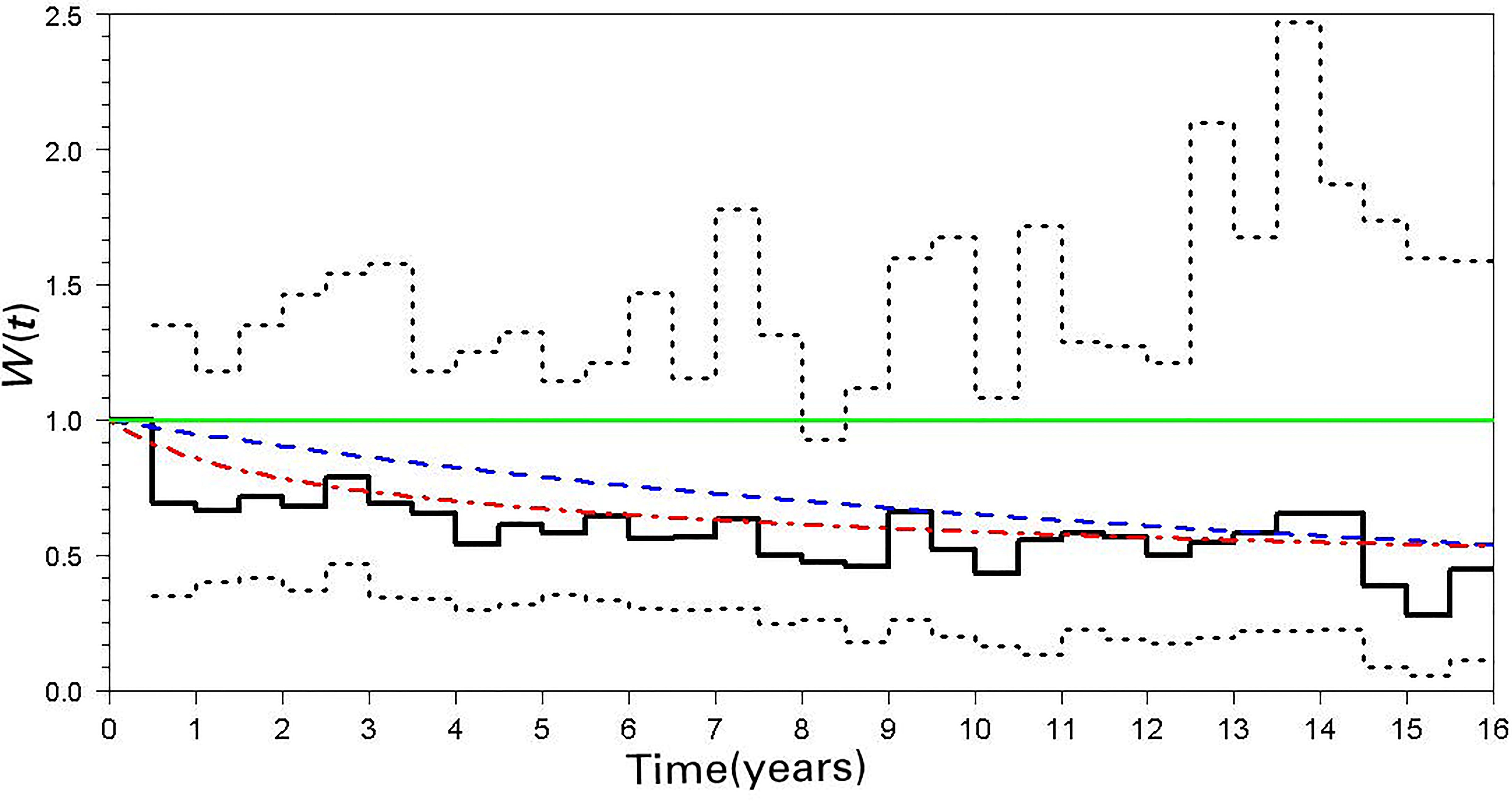
Estimates of the nonstationarity function ( $W(t)$ ) versus time for MACS data. Solid line: UMCAD (step function); dotted lines: lower and upper 95% confidence bounds; dashed line: SMCAD-alternative function; line with alternating dashes and dots: SMCAD-Zimmerman and Núñez-Antón function.

The within-person correlation structure of the CD4 count over time, with a focus on the pattern of nonstationarity, was studied by fitting UMCAD and SMCAD models to the data. Residuals were obtained by correcting for the sample mean and standard deviation for measurements at each time point; the $R_{ij}$ outcomes were then computed using the ‘variogram’ definition mentioned above. As there are 33 distinct time points over the sample, the UMCAD model involves 32 correlations. The NLLS method was used to estimate the UMCAD correlations and the step-function for $W(t)$ . The estimated correlation for the first interval (0 to 6 months), which was used as the reference, was 0.63. Figure 3 provides the plot of the estimated $W(t)$ versus time from HIV seroconversion, along with nonparametric 95% confidence bounds (obtained as described in Section 3.2.3). As shown in the figure, there was a slight decrease in the estimated $W(t)$ over time, indicating increasing time expansion (and higher correlations for equally spaced intervals) over the observation period. Although, the (upper) 95% confidence interval bound crosses the line $W(t)=$ 1, it barely does so, suggesting marginal evidence for nonstationarity.

In addition, two SMCAD models were fit to the data. The first model, derived from the Zimmerman and Núñez-Antón (ZN) correlation function (given in Section 2), can be represented by the nonstationarity function $W(t;\lambda)=(t+1)^{\lambda-1}$ . The slight modification to the ZN function is the translation from $t$ to $t+1$ , the purpose of which was to obtain the constraint $W(0)=$ 1 as used in the UMCAD. An alternative model, suggested by the plot of the estimated $W(t)$ for the UMCAD, is $W(t;\lambda)=1/(1+\lambda t)$ . This nonstationarity function corresponds to the correlation function, $\phi(t_{j},t_{k};\lambda)\equiv\rho^{[\log(1+\lambda t_{k})-\log(1+\lambda t_{% j})]/\lambda}$ . This alternative function is more specialized in that it only accommodates time expansion (increasing correlations over time) but not time contraction. Consequently, this model is not useful for testing for nonstationarity. The two estimated functions are also plotted in Fig. 3. For these data, the ZN function appears to more closely fit the step-function estimate of $W(t)$ as well as providing a better fit according to the NLLS criterion Eq. (6). The estimated $\lambda$ ’s (and 95% confidence intervals) are 0.78 (0.66, 0.90) for the ZN model and 0.054 (0.016, 0.091) for the alternative model, respectively. The positive estimates for $\lambda$ in both structured models suggest time expansion with increasing time from seroconversion. Also, as the CI for $\lambda$ for the SMCAD model with the ZN function excludes 0, there is evidence for nonstationarity of the correlation structure based on this model.

5. Simulation study

5.1 Study design

Simulation studies were conducted to compare the proposed NLLS and a maximum likelihood approach to estimation of UMCAD model parameters under different scenarios, including varying sample sizes and extent of data sparseness. Data were simulated to resemble the calf data analyzed previously by Kenward (1987), as this example provided a convenient reference with a modest number of measurement times. Specifically, (11 $\times$ 1) residuals vectors for each subject were generated independently from a multivariate normal distribution with first-order antedependence covariance structure, and using a zero mean vector and variances equal to the (time-by-time) sample estimates from the calf data. (These values are in code provided by request.) The specified UMCAD model correlation values were taken as similar to those estimated from the calf data, namely, $(\rho_{1},\ldots,\rho_{10})=$ (0.82, 0.91, 0.93, 0.94, 0.94, 0.93, 0.93, 0.97, 0.96, 0.98).

Four sample sizes were used: 30, 100, 300, and 500. In addition, sparse data scenarios were created by random deletion of observations (independently for each observation with a fixed probability, denoted as $p$ ). Four deletion probabilities were used: 0 (complete data case), 0.6, 0.75, and 0.90. For each of these 16 (4 $\times$ 4) scenarios, 300 replicate data sets were generated. An alternative missing data mechanism was also considered in which missingness was produced by constrained randomization, so that the exact targeted proportion of missing observations (0. 0.6, 0.75, and 0.9 as before) was obtained at each time point. The same initial sample sizes and estimation methods were used as in the unconstrained randomization approach. For each dataset, the UMCAD model correlations were estimated using both the MLE and the proposed NLLS methods. Both approaches (correctly) assumed a null mean structure and unstructured variances over time. The MLE approach simultaneously estimated the mean (including only time as a categorical variable) and covariance parameters, while the NLLS approach used the residuals based on sample estimates of the mean and standard deviation at each time point, with outcomes constructed as products of adjacent residuals.

Table 1
Bias, MSE for maximum likelihood (MLE) and nonlinear least squares (NLLS) estimators from simulations for each correlation parameter in UMCAD model for complete data and 60% missing scenarios. Sample size $=$ 30

Par	Bias	% Bias	MSE	Bias	% Bias	MSE	Bias	% Bias	MSE	Bias	% Bias	MSE
	Complete data						60% missing
	MLE			NLLS			MLE			NLLS
$\rho_{1}$	$-$ 0.0042	$-$ 0.51	0.0043	0.0024	0.30	0.0021	$-$ 0.012	$-$ 1.42	0.0156	0.0024	0.29	0.0051
$\rho_{2}$	$-$ 0.0051	$-$ 0.56	0.0013	$-$ 0.0001	$-$ 0.008	0.0005	$-$ 0.0039	$-$ 0.42	0.0046	0.0019	0.21	0.0014
$\rho_{3}$	$-$ 0.0027	$-$ 0.29	0.0009	0.0008	0.089	0.0004	$-$ 0.0087	$-$ 0.94	0.0029	$-$ 0.0033	$-$ 0.36	0.0009
$\rho_{4}$	$-$ 0.0035	$-$ 0.37	0.0005	$-$ 0.002	$-$ 0.21	0.0002	$-$ 0.0068	$-$ 0.72	0.0038	$-$ 0.0002	$-$ 0.025	0.0006
$\rho_{5}$	$-$ 0.0025	$-$ 0.27	0.0005	$-$ 0.0013	$-$ 0.14	0.0003	$-$ 0.0063	$-$ 0.67	0.002	0.0014	0.15	0.0006
$\rho_{6}$	$-$ 0.0015	$-$ 0.16	0.0007	$-$ 0.0003	$-$ 0.03	0.0003	$-$ 0.0032	$-$ 0.35	0.0021	0.0023	0.24	0.0008
$\rho_{7}$	0.0002	0.026	0.0007	0.0015	0.16	0.0003	$-$ 0.0046	$-$ 0.50	0.0019	0.001	0.10	0.0008
$\rho_{8}$	0.0001	0.015	0.0001	0.0009	0.093	0.0001	$-$ 0.0015	$-$ 0.16	0.0004	0.0005	0.049	0.0001
$\rho_{9}$	$-$ 0.0014	$-$ 0.15	0.0003	0.0002	0.019	0.0001	$-$ 0.0027	$-$ 0.28	0.0009	0.0011	0.11	0.0003
$\rho_{10}$	$-$ 0.0001	$-$ 0.013	0.0001	0.0005	0.051	$<$ 0.0001	$-$ 0.0011	$-$ 0.11	0.0002	0.0001	0.0056	0.0001
Ave	0.0021	0.24	0.0009	0.001	0.11	0.0004	0.005	0.56	0.0034	0.0014	0.15	0.0011

Note: MLE and NLLS converged in all 300 simulation runs for complete data; MLE converged in 279 and NLLS converged in all 300 simulations for 60% missing data simulations.

Because the simulated data involved a relatively small number of distinct times points (namely 11), and thus a similarly small number of UMCAD correlations (10 $=11-1$ ), the properties of the MLE and NLLS estimators were examined for each of these correlation parameters. Denoting $\hat{\rho}_{k}$ as the mean simulation estimate (of the corresponding correlation, $\rho_{k}$ , $k=$ 1, …, 10) over the 300 replicate samples, the following statistics were computed for each estimator: bias ( $B=\hat{\rho}_{k}-\rho_{k}$ ), percent bias ( $100\cdot B/\rho_{k})$ , and mean squared error (MSE). In addition, measures of overall bias, relative bias and overall efficiency were obtained by averaging the absolute values of the biases, relative biases and MSEs, respectively, over the 10 correlations. In another set of simulations we compared estimated versus true (simulated) standard errors as well as coverage of confidence intervals. Computed statistics (for each correlation and overall) included the average estimated standard error, the simulation (‘true’) standard estimate (obtain as the empirical standard deviation over the simulations), and coverage (percent of 95% confidence intervals covering the true value). Data were generated and analyzed using SAS Version 9.2 (SAS Institute Inc., Cary, NC, USA). The MLE method was implemented using PROC MIXED and the NLLS method was implemented using SAS/IML and PROC NLP.

5.2 Simulation study results

Simulation study results for $n=$ 30 and for $p=$ 0 and 0.6 are provided in Tables 1 and 2. Results for other scenarios are summarized below and can be provided upon request. As seen in Table 1, both methods showed low relative bias (less than 1 percent in absolute value) for all correlation parameters and all sample size scenarios in the complete data ( $p=$ 0) case. For the small sample case ( $n=$ 30), the average (absolute value of the) bias is lower for the NLLS than the MLE method for all deletion probabilities where results are obtained, with the relative advantage of the NLLS method over MLE increasing with increasing $p$ . For example, for the MLE and NLLS methods, respectively, the average (absolute value of) relative biases are 0.24 and 0.11 percent for $p=$ 0, and 0.56 and 0.15 percent for $p=$ 0.6. In the case of $n=$ 30, with $p$ equal to 0.75 or 0.9, the MLE failed to converge in nearly all of the 300 simulated data sets for each scenario, while the NLLS converged in all of them. Even in these high sparseness cases, the NLLS showed less than 1% (absolute value of) relative bias for all but two correlations (which still had less than 1.2% relative bias). Table 2 indicates that standard errors for both the NLLS and MLE methods are generally under-estimated, and consequently there is often under-coverage of confidence intervals. MLE appears to perform better in the complete data case, while the NLLS method shows closer to nominal coverage in the case of irregular data (60% missing).

For the larger sample size of 100, similar trends were found, with lower average (absolute value of) relative biases for NLLS relative to MLE for all values of $p$ , and the advantage of NLLS increasing for increasing $p$ . For $n=$ 100, both methods converged in all 300 simulations up to $p=$ 0.75, while the NLLS converged for all 300 and the MLE did not converge for any when $p=$ 0.9. For sample sizes of 300 and 500 both methods showed low relative bias for all correlations for all values of $p$ , though the MLE still failed to converge in a higher proportion of simulations at $p=$ 0.9. Still, the results in all scenarios (using the simulations where the MLE converged) showed a smaller average relative bias for the NLLS than the MLE method. For estimation of standard errors and coverage of confidence intervals, similar patterns as noted above were found for larger sample sizes and higher proportions of missing.

Table 2
Standard error, coverage (percent) for maximum likelihood (MLE) and nonlinear least squares (NLLS) estimators from simulations for each correlation parameter in UMCAD model for complete data and 60% missing scenarios. Sample size $=$ 30

	Complete data						60% Missing
	MLE			NLLS			MLE			NLLS
Par	S.E.	Simulated S.E.	Cover (%)	S.E.	Simulated S.E.	Cover (%)	S.E.	Simulated S.E.	Cover (%)	S.E.	Simulated S.E.	Cover (%)
$\rho_{1}$	0.0607	0.0660	90.67	0.0448	0.0660	82.67	0.1021	0.2087	71.43	0.1274	0.1503	86.67
$\rho_{2}$	0.0322	0.0354	89.33	0.0227	0.0354	79.33	0.0533	0.1293	69.31	0.0889	0.0993	90.00
$\rho_{3}$	0.0257	0.0267	93.00	0.0180	0.0267	81.00	0.0429	0.0770	69.31	0.0730	0.0757	86.00
$\rho_{4}$	0.0217	0.0210	92.00	0.0151	0.0210	82.67	0.0373	0.0915	76.19	0.0678	0.0739	83.67
$\rho_{5}$	0.0223	0.0237	92.67	0.0155	0.0237	81.33	0.0324	0.1004	66.14	0.0658	0.0721	85.67
$\rho_{6}$	0.0258	0.0276	91.00	0.0180	0.0276	82.67	0.0383	0.0841	70.37	0.0646	0.0718	86.00
$\rho_{7}$	0.0266	0.0337	91.67	0.0185	0.0337	78.33	0.0369	0.0675	77.25	0.0639	0.0681	90.67
$\rho_{8}$	0.0115	0.0148	90.33	0.0079	0.0148	75.67	0.0192	0.0851	65.08	0.0540	0.0672	78.00
$\rho_{9}$	0.0149	0.0161	92.67	0.0102	0.0161	81.00	0.0218	0.0862	71.96	0.0578	0.0717	81.33
$\rho_{10}$	0.0076	0.0098	90.33	0.0053	0.0098	78.00	0.0146	0.0898	65.08	0.0508	0.0773	68.33
Ave	0.0249	0.0533	91.37	0.0176	0.0533	80.27	0.0399	0.1170	70.21	0.0714	0.0954	83.63

Note: MLE and NLLS converged in all 300 simulation runs for complete data; MLE converged in 189 and NLLS converged in all 300 simulations for 60% missing data simulations.

6. Conclusion

This paper presents a new continuous-time nonstationary (antedependence) covariance model for repeated measures data. This model introduces a useful nonstationarity function which describes changes in local correlations as a function of time. Both unstructured and structured versions of the model were presented. A novel approach to estimation was presented that uses a nonlinear regression model formulation leading to nonlinear least squares estimators of model parameters and nonparametric and parametric confidence intervals. Sample SAS code, implementing the proposed method for the MACS data, is available upon request.

Simulation studies show advantages of the new NLLS method over the standard MLE approach in reducing bias of correlation parameter estimates, with the advantage increasing with increasing data sparseness. Furthermore, in a number of scenarios, a standard algorithm for ML estimation failed to converge, while the NLLS method converged in all cases. A limitation of the above conclusions is that the MLE approach studied involved a particular (albeit popular) algorithm, as implemented in the SAS Mixed Procedure. The convergence problems that we observed are not connected to non-identifiability, but are due to numerical problems that tend to occur in the case of sparse and unbalanced data. It is possible that an alternative algorithm could improve on the convergence rates obtained here.

Sparseness in practice may involve different patterns and mechanisms. For example, a higher proportion of missingness may be expected at later follow-up times. The unconstrained and uniform probability mechanism used for generating missingness provided a simple first approach for the simulation study. As described above, additional simulations were conducted under an alternative mechanism involving constrained random deletions that produced a fixed proportion of missing values at each time. Not surprisingly, given the greater regularly of data patterns produced, this situation somewhat decreases the advantage of the NLLS over the MLE approach, though the former is still superior in terms of bias and convergence for very sparse scenarios. On the other hand, only multivariate normally distributed responses were considered in the present simulation studies. A comparison of the methods using non-normally distributed data may be expected to show an even greater advantage of the NLLS over the MLE method, as the former does not make any distributional assumption. Finally, an assumption of the proposed estimators is that missingness is completely at random. It would be of interest to study and possibly extend the proposed methodology for contexts where missingness may be informative.

Simulation results indicated that standard errors for both the NLLS and MLE methods were under-estimated and consequently that confidence intervals for UMCAD correlation parameters showed pronounced under-coverage, though the performance of the NLLS method improved somewhat in irregular data scenarios. For the NLLS method under-estimation of standard errors may be due to inadequately accounting for estimation of mean parameters. Further research is needed to refine the NLLS standard error estimators; alternatively, a bootstrap resampling approach for standard errors and confidence intervals may be considered.

Both the data example and simulation studies focused on an unweighted estimator, though a weighted approach is possible. The unweighted estimator is appealing given its good finite sample properties (including low bias) and greater simplicity. Nevertheless, possible improved efficiency of the weighted estimator under various scenarios could use further study. Another limitation was the restriction to a Markovian model, which also assumes an absence of measurement error. An extension to a more general non-Markovian continuous antedependence model is possible and is left for future research.

The proposed continuous antedependence model and estimation approach may be useful even where the mean structure is of primary interest (as in some previous studies using antedependence covariance models, e.g., Hou et al. (2006)). Although the present paper gave little attention to inference for the mean structure, a joint consideration of the mean and covariance structures in the continuous time and sparse data context will be of interest.

The present exposition of the nonstationarity function in terms of an expansion or contraction of time provides the function with an elegant and scientifically interesting interpretation. The nonstationarity function may also be viewed as describing informativeness of additional measurements over time. Thus, the CAD analysis, and resulting estimate of the nonstationarity function, may be useful for designing – in particular, choosing measurement times for – repeated measures studies. Optimal design based on the nonstationarity function is a topic for future research.

Footnotes

Acknowledgments

This work was supported by the National Institute of Dental and Craniofacial Research, National Institutes of Health [grant number: R01DE025835 (J. Albert)].

References

Albert

J.M.

(1992). A corrected likelihood ratio statistic for the multivariate regression model with antedependent errors. Communications in Statistics – Theory and Methods, 21, 1823-1843.

Al- Ibrahim

A.H.

(1999). A variance components model for analyzing repeated measures designs with non-stationary error structure. Biometrical Journal, 41, 573-582.

Boscardin

W.J.

Taylor

J.M.G.

, & Law

(1998). Longitudinal models for AIDS marker data. Statistical Methods in Medical Research, 7, 13-27.

Byrne

P.J.

, & Arnold

S.F.

(1983). Inference about multivariate means for a nonstationary autoregressive model. Journal of the American Statistical Association, 78, 850-855.

Diggle

P.J.

Heagerty

Liang

K.-Y.

, & Zeger

S.L.

(2002). Analysis of Longitudinal Data (2nd ed). New York: Oxford University Press.

Diggle

P.J.

, & Verbyla

A.P.

(1998). Nonparametric estimation of covariance structure in longitudinal data. Biometrics, 54, 401-415.

Gabriel

K.R.

(1961). The model of ante-dependence for data of biological growth. Bulletin de l’Institut International Statistique (Paris), 39, 253-264.

Gabriel

K.R.

(1962). Ante-dependence analysis of an ordered set of variables. Annals of Mathematical Statistics, 33, 201-212.

Hou

Garvan

C.W.

, & Zhao

(2006). A general likelihood model for characterizing cocaine-induced genetic determinants for developmental trajectories in early childhood. Statistics in Medicine, 25, 4020-4035.

10.

Jacqmin-Gadda

Joly

Commenges

Binquet

, & Chêne

(2002). Penalized likelihood approach to estimate a smooth mean curve on longitudinal data. Statistics in Medicine, 21, 2391-2402.

11.

Kaslow

R.A.

Ostrow

D.G.

Detels

Phair

J.P.

Polk

B.F.

, & Rinaldo

C.R.

, Jr. (1987). The multicenter AIDS cohort study: Rationale, organization, and selected characteristics of the participants. American Journal of Epidemiology, 126, 310-318.

12.

Kenward

M.G.

(1987). A method for comparing profiles of repeated measurements. Applied Statistics, 36, 296-308.

13.

Krzanowski

W.J.

(1999). Antedependence models in the analysis of multi-group high-dimensional data. Journal of Applied Statistics, 26, 59-67.

14.

Macchiavelli

R.E.

, & Arnold

S.F.

(1994). Variable order ante-dependence models. Communications in Statistics – Theory and Methods, 23, 2683-2699.

15.

Macchiavelli

R.E.

, & Moser

E.B.

(1997). Analysis of repeated measurements with ante-dependence covariance models. Biometrical Journal, 39, 339-350.

16.

Núñez-Antón

(1998). Longitudinal data analysis: Non-stationary error structures and antedependent models. Applied Stochastic Models and Data Analysis, 13, 279-287.

17.

Núñez-Antón

, & Woodworth

G.G.

(1994). Analysis of longitudinal data with unequally spaced observations and time-dependent correlated errors. Biometrics, 50, 445-456.

18.

Núñez-Antón

, & Zimmerman

D.L.

(2000). Modeling nonstationary longitudinal data. Biometrics, 56, 699-705.

19.

Patel

H.I.

(1991). Analysis of incomplete data from a clinical trial with repeated measurements. Biometrika, 78, 609-619.

20.

Rubin

D.B.

(1976). Inference and missing data. Biometrika, 63, 581-592.

21.

Struthers

C.A.

, & McLeish

D.L.

(2011). A particular diffusion model for incomplete longitudinal data: Application to the multicenter AIDS cohort study. Biostatistics, 12, 493-505.

22.

Taylor

J.M.G.

, & Law

(1998). Does the covariance structure matter in longitudinal modelling for the prediction of future CD4 counts? Statistics in Medicine, 17, 2381-2394.

23.

Zhang

(2005). Multiple imputation of missing data with ante-dependence covariance structure. Journal of Applied Statistics, 32, 141-155.

24.

Zimmerman

D.L.

, & Núñez-Antón

(1997). Structured antedependence models for longitudinal data. Modelling Longitudinal and Spatially Correlated Data: Methods, Applications, and Future Directions Gregoire

T.G.

Brillinger

D.R.

Diggle

P.J.

Russek-Cohen

Warren

W.G.

, & Wolfinger

(eds), New York: Springer-Verlag, 63-76.

25.

Zimmerman

D.L.

, & Núñez-Antón

V.A.

(2009). Antedependence Models for Longitudinal Data. Chapman and Hall/CRC.

26.

Zimmerman

D.L.

Núñez-Antón

, & El-Barmi

(1998). Computational aspects of likelihood-based estimation of first-order antedependence models. Journal of Statistical Computation and Simulation, 60, 67-84.

Continuous time nonstationary correlation models for sparse longitudinal data

Abstract

Keywords

1. Introduction

2. Background: Discrete antedependence

3.1 Model

3.2.1 Setup

3.2.2 Nonparametric estimation for the MCAD

3.2.4 Structured MCAD (SMCAD) model estimation

5.1 Study design

Table 1 Bias, MSE for maximum likelihood (MLE) and nonlinear least squares (NLLS) estimators from simulations for each correlation parameter in UMCAD model for complete data and 60% missing scenarios. Sample size = 30

Table 2 Standard error, coverage (percent) for maximum likelihood (MLE) and nonlinear least squares (NLLS) estimators from simulations for each correlation parameter in UMCAD model for complete data and 60% missing scenarios. Sample size = 30

Footnotes

Acknowledgments

References

Table 1
Bias, MSE for maximum likelihood (MLE) and nonlinear least squares (NLLS) estimators from simulations for each correlation parameter in UMCAD model for complete data and 60% missing scenarios. Sample size $=$ 30

Table 2
Standard error, coverage (percent) for maximum likelihood (MLE) and nonlinear least squares (NLLS) estimators from simulations for each correlation parameter in UMCAD model for complete data and 60% missing scenarios. Sample size $=$ 30