In the statistical analysis of bivariate data, it is possible to have discrete observations instead of continuous data, as observed in many studies with survival data. In this study it is introduced a new bivariate discrete distribution derived from two Rayleigh distributions using a method proposed by Marshall and Olkin (1997) where an additional parameter is is introduced to a family of distributions related to the dependence structure of two discrete random variables and . The study results show that this new bivariate distribution has good statistical properties and a simple mathematical expression for its correlation coefficient. The usual classical and Bayesian estimators for the parameters of the new distribution are also presented. A simulation study is carried out in order to evaluate some frequentist properties of the proposed model. The usefulness of the proposed model is illustrated using a real medical dataset introduced in the literature in presence of censoring and covariates.
The introduction of new survival distributions has been the objective of many studies introduced in the literature since this class of models is widely used in many areas of application, especially in medical or engineering studies where the lifetimes usually are measured in a continuous scale. However, in many applications, it is possible to have the observed responses measured in a discrete scale where it is not appropriate to assume the data as continuous data. Nevertheless, in many applications despite the discrete data, it is common to use continuous models due to model analytical tractability or facilities in obtaining parameter estimators using existing statistical software where the most popular continuous lifetime distributions usually are implemented. However, this procedure may not be appropriate in many applications as it may be impossible to measure the lifetime of a component on a continuous scale, as in the on/off switching devices, number of cycles until failure, or the number of accidents in a road (see for example, Kundu, 2014, 2017; Kundu et al., 2010; Kundu & Gupta, 2009; Kundu & Nekoukhou, 2018).
As more specific examples of lifetime applications, we could consider the times of deterioration levels, the times of infection or the times to reaction for a treatment in pairs of lungs, kidneys, eyes or ears of humans that could be given as count of the number of days, weeks or months. In this case, the use of a continuous distribution could lead to inaccurate inference results which is a great motivation to introduce new and more flexible discrete bivariate lifetime distributions together with their mathematical properties and inference results. In this direction special attention has been given on bivariate geometric distributions and bivariate Poisson distributions (see for example Kocherlakota S & Kocherlakota K, 1992; Kocherlakota, 1995; Arnold, 1975; Basu & Dhar, 1995; Kumar, 2008; Kemp, 2013; Lee & Cha, 2014; Nekoukhou & Kundu, 2017; Kundu & Nekoukhou, 2018) as alternatives to many bivariate continuous models introduced in the literature (see for example, Block & Basu, 1974; Marshall & Olkin, 1967a,b; Downton, 1970; Freund, 1961; Sarkar, 1987; Arnold & Strauss, 1988; Gumbel, 1960; Hanagal, 2006; Hanagal & Ahmadi, 2008; Hawkes, 1972; Hougaard, 1986; Balakrishnan & Lai, 2009; Popović & Genç, 2018).
In some cases, the bivariate distributions of survival data introduced in the literature may present inconvenient forms to be used in applications, as the two classes of discrete bivariate distributions introduced by Lee and Cha (2014), although the motivation for this model to be quite simple based on the minimum and maximum of two different independent random variables. In this model there are great difficulties to calculate the estimators of the unknown parameters and to determine their properties (see also, Nekoukhou & Kundu, 2017).
From these considerations, there is a great motivation to introduce new bivariate lifetime distributions with simple mathematical properties and simplifications to get the inferences of interest, the main goal of this study. In this direction, this paper introduces a new discrete bivariate Rayleigh distribution obtained by using a procedure introduced by Marshall and Olkin (1997) where the marginal distributions are discrete generalized Rayleigh distributions implying in great model flexibility for the hazard function, which could be given by bathtub, increasing and increasing-decreasing-increasing shapes depending on the parameter values. This paper also introduces a multivariate extension of the proposed bivariate model. An additional justification for the use of bivariate survival distributions is the possible simplification of the mathematical expression for the likelihood function in the presence of censored data, a common situation in lifetime data applications as in medical or engineering studies, when compared to some existing continuous bivariate lifetime distributions where the likelihood function in presence of censored data usually depends on joint survival functions given in non-analytical mathematical forms.
In the construction of bivariate probability distributions, especially for the continuous case, the literature presents many different techniques such as: the use of copula functions, mixing and compounding; the use of trivariate reduction; the specification of a conditional and a marginal distribution; the use of a conditionally method; the construction of discrete bivariate distributions with specified marginals and correlation; the use of sums and limits of Bernoulli random variables; the use of clusters; the construction of finite bivariate distributions via extreme points using convex sets; the use of generalized distributions methods; the use of canonical correlation coefficients and semi-groups; the use of bivariate distributions generated from weight functions; the use of marginal transformation methods; the use of truncation or the use of two-stage failure risks of a two-component parallel system method (see Kocherlakota S & Kocherlakota K, 1992; Lai, 2006; Balakrishnan and Lai, 2009). However, unlike their continuous analogues, discrete bivariate distributions usually are harder to be constructed. Kemp and Papageorgiou (1982) pointed out that the main problem in the construction of bivariate distributions is the impossibility to have a standard set of criteria that can always be applied to produce a unique bivariate distribution obtained from an univariate distribution which could unequivocally be called the bivariate version.
Meanwhile, Marshall and Olkin (1997) introduced a method to obtain an extended family of distributions including one additional parameter denoted as univariate Marshall-Olkin family having cumulative distribution function and survival function given, respectively, by,
where , , and . This new family of distributions has an additional parameter which generalizes the baseline distribution and is related to the dependence structure of two random variables. This family could also be extended to the multivariate case. In this way, let be a random vector with multivariate cumulative and survival functions given, respectively, by and ; the multivariate Marshall-Olkin family has cumulative distribution function and survival function given, respectively, by,
where and . Notice that the functions obtained in Eq. (2) are more flexible than the functions obtained from the product of independent distributions providing a great flexibility in the modeling of the dependence structure.
The main goal of this paper is to introduce a new bivariate discrete distribution with great flexibility for the correlation coefficient range and to avoid not very accurate inferential results usually obtained using other existing bivariate lifetime models. In this way, the Marshall and Olkin (1997) method is considered in this study in the construction of a bivariate discrete distribution due to its flexibility to introduce a new parameter related to the dependence of the two random variables and . The Rayleigh distribution is also used to compose the bivariate model due to its great applicability to reliability and survival medical data. In this way, the resulting distribution could be a good alternative to other existing bivariate discrete distributions introduced in the literature.
This paper is organized as follows: Section 2 presents the bivariate discrete generalized Rayleigh distribution and its basic properties. The structural properties including the mean, variance, the dependence structure, a formula to compute bivariate probabilities and its implementation are also presented in Section 2. Maximum likelihood and Bayesian estimators for the parameters of the proposed model are presented in Section 3. Section 4 presents the results of a simulation study; Section 5 presents two applications considering bivariate medical survival data. Finally, Section 6 closes the paper with some concluding remarks.
Bivariate discrete generalized rayleigh distribution
Model description
Let be two independent discrete random variables having Rayleigh distributions (see Roy, 2004) with parameters . Since are independent random variables, the joint survival function of the bivariate random variables and is given by,
Observe that the joint survival function in Eq. (3) is restricted to independent lifetimes and cannot be applied directly assuming dependence structures in bivariate data. In this way, using the Marshall-Olkin survival function given in Eq. (2), the new proposed joint survival function is given by,
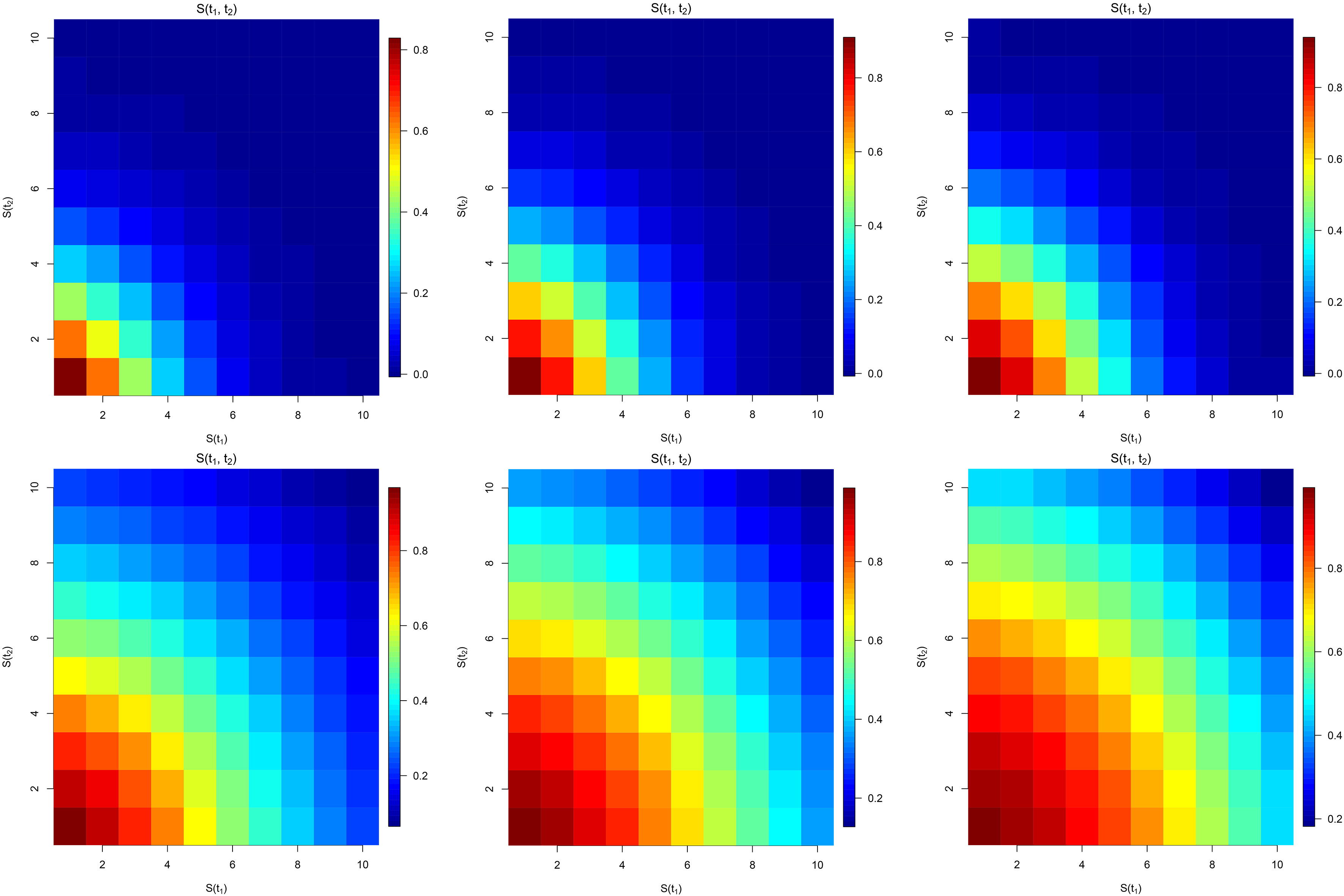
where and . Observe that Eq. (4) is more flexible than Eq. (3) and can be applied directly to model the dependence structure for correlated bivariate lifetimes. The joint survival function defined by Eq. (4) is denoted as a bivariate discrete generalized Rayleigh (BDGR) distribution and special cases of its contour plot are illustrated in Fig. 1, assuming different values for the parameters and .
Discrete contour plots of the joint survival function for the BDGR model assuming different parameter values (Upper-panels: fixed values given by 0.95, and 0.50 1.00 1.50s. Lower-panels: fixed values given by 0.99, and 0.50 1.00 1.50).
.
Let be a discrete random vector following the joint survival function given by Eq. (4) with parameters and . Defining , , the joint probability mass function (pmf) of is given by,
where ; ; ; and denotes a univariate discrete Rayleigh distribution. Observe that Eq. (5) is a proper joint pmf since the series expressed by converges to for where is the Jacobi theta function.
Marginal and conditional distributions
For the Bivariate Discrete Generalized Rayleigh Distribution, the marginal distributions of the random variables and are given by discrete generalized Rayleigh (DGR) distributions with corresponding parameters and , respectively. Many properties of the continuous generalized Rayleigh distribution were introduced by MirMostafaee et al. (2017). Since the DGR inherits most of the properties of the continuous model in the univariate case, these marginals have great flexibility for the hazard function, given by bathtub, increasing and increasing-decreasing-increasing shapes depending on the parameter values. In this way, this bivariate distribution could be very useful especially to model positive data. The marginal survival and marginal pmf functions can be expressed, respectively, by,
The mean expected value and variance for the marginal probability distributions do not have closed forms, however they could be computed using numerical methods from the mean and variance around the origin given by,
which could be approximated using the finite series given by:
Now, let us assume the transformation of the random variables and given by . In this case, the cumulative probability function of the random variable W is given by,
which implies that the distribution of is a discrete generalized Rayleigh (DGR) distribution with parameters . The mean expected value and variance could also be approximated by the finite series given in Eq. (6).
For the BDGR model, the conditional distribution of given and is given by,
Covariance and correlation coefficient
For the BDGR distribution given by Eq. (5), the cross factorial moment between and is given by,
which is a monotonic increasing function of and since,
for . However, the cross factorial also could be approximated using series representation of the logarithmic function. That is, suppose that is an integer sufficiently large and ; thus, we have,
which is a finite series and can be determined when the parameters of the distribution are estimated from a dataset.
.
(Covariance signal) Let the covariance signal be defined by the function,
thus if , if and if . That is, the covariance signal only depends on the parameter .
Proof..
Note that the function is a continuous function on and its first derivative is given by,
Note that, since and , then if . On the other hand, if then ; if then and the proof is complete. ∎
From the function given in Eq. (8), the proposed model admits a very flexible behavior for the correlation coefficient of any sign. In fact it is observed that if , and if . If the correlation coefficient is equal to zero. Although there is no closed form for the expressions of the covariance and correlation coefficient these expressions could be computed by taking a large number of terms in the series defined in Eq. (6). Table 1 presents the approximated results for the covariance and correlation coefficients for some fixed values of and from which can be seen the flexibility of the correlation coefficient .
Theoretical results under a BDGR distribution
(0.2, 0.2, 0.2)
0.0084
0.0061
0.1281
(0.8, 0.2, 0.2)
0.0327
0.0046
0.0310
(0.5, 0.5, 0.5)
0.1777
0.0433
0.0980
(1.0, 0.5, 0.5)
0.3186
0.0000
0.0000
(1.2, 0.5, 0.5)
0.3676
0.0191
0.0267
(1.5, 0.5, 0.5)
0.4348
0.0466
0.0579
(1.8, 0.8, 0.8)
2.6964
0.2225
0.0298
(2.0, 0.8, 0.8)
2.8597
0.2721
0.0342
Special cases and multivariate extension
.
(Special cases) Some especial cases of the BDGR are given by,
If , the pmf of BDGR is symmetric in its arguments, that is, for all .
If , the pmf of BDGR is also symmetric in its arguments and its reduced to a one parameter bivariate discrete distribution with probability mass function given by,
If and , the pmf of BDGR can be rewritten as an infinite mixture of the product of two Rayleigh distributions.
Proof..
(i) and (ii) are trivial. For (iii), the result is obtained by considering the series representation,
and noticing that . ∎
.
(Multivariate extension)Let be independent discrete random variables having the Rayleigh distribution with parameters . Since are independent, the multivariate survival and multivariate pmf functions are given, respectively by,
and,
For the multivariate model, the dependence among the n lifetimes is specified by the parameter , where if there is independence among the n lifetimes. The model adequacy could be checked by comparisons of the fitted marginal survival functions with the empirical estimates of the marginal survival distributions since the marginal survival functions are discrete generalized Rayleigh distributions as well. Moreover, the correlation coefficient for the multivariate case has the same properties of the correlation coefficient of the bivariate model, that is, it could be negative, positive or equal to zero. Since extensive calculations are required for the multivariate case, their properties are not derived here.
Inference methods
Maximum likelihood approach
This section introduces the maximum likelihood estimation (MLE) method in two situations: the situation assuming censored data and the situation with complete data. In both cases, the maximum likelihood estimators do not have closed forms requiring the use of numerical methods like Newton-Raphson or Nelder-Mead to get the estimators for each parameter.
Complete data
Let be a random sample of size from a BDGR distribution. The log-likelihood function is given by:
The normal equations (the partial derivatives of the log-likelihood function with respect to the parameters are equal to zero) obtained from Eq. (13), are not reproduced here as they cannot be solved explicitly. They must be solved either by numerical methods as, for example, the Newton-Raphson optimization method or by directly maximization of the log-likelihood function. Since the global maximum of the log–likelihood surface is not guaranteed, different initial values in the parameter space sould be considered as seed points. From the log-likelihood function, the first derivatives of with respect to and are given, respectively by
Under standard asymptotic maximum likelihood theory, a consistent estimator for the covariance matrix of is obtained by the inverse of the expected Fisher information matrix of , evaluated at . In this case, the Fisher information could be approximated by the observed Fisher information matrix where its elements are given by the second derivatives of the log-likelihood function with respect to and locally at the obtained MLE’s. Hypothesis testing and confidence intervals for and could be obtained by using the asymptotical normality (see Lawless, 1982) of the MLEs and , that is,
where is the observed Fisher information matrix.
Censored data
In many applications related to lifetime data there is the presence of censored data, that could be right, left or interval censoring. In this section, let us assume the presence of right censored data, that is, associated to each lifetime , there is a fixed censoring time and the data are given by and . The likelihood function for the parameters of the BDGR distribution based on a sample of size n has the dataset classified in four regions:
: Both, and , are complete observations;
: are complete and are censored;
: are censored and are complete;
: Both, and , are censored observations.
Thus, the likelihood function for and based on bivariate observations is given by,
where and . Let us also define the following indicator variables of censoring,
where are the right censoring times. From Eq. (16) are obtained the following results needed for the likelihood function:
For , we have,
For , we have,
For , we have,
For , we have,
Remark 1 The dependence between the two lifetimes is specified by the parameter , where if there is independence between the two lifetimes. The adequacy of the marginal distributions in presence of censored data could be verified by plots of the fitted survival functions and non-parametric Kaplan-Meier estimates for the survival function. In situations not considering censored data is used standard empirical estimates of the survival function.
A Bayesian approach
The Bayesian paradigm is based on specifying a probability distribution for the observed data given a vector of unknown parameters (assuming as a vector of random variables) providing a rational method for updating the new information using the Bayes’ rule given the prior distribution specifying the uncertainty about the parameter (see Ibrahim et al., 2005).
In the determination of the Bayes estimators for the unknown parameters of the BDGR model based on the squared error loss function, , suppose that the parameters and have independent Beta() and flat (improper) prior distributions given respectively, by,
The joint posterior density function for the parameters and of the proposed BDGR distribution is obtained directly from the Bayes formula, that is,
Therefore, the Bayes estimator of any function of , and , say , assuming the squared error loss function is given by,
Given the difficulties in analytically finding the Bayesian estimators of interest given by expression Eq. (19), MCMC (Markov Chain Monte Carlo) methods are used to get the posterior summaries of interest (see, for example, Gelfand & Smith, 1990; Chib & Greenberg, 1995; Achcar & Leandro, 1998). In this way, assuming the BDGR distribution for the bivariate lifetime data, Monte Carlo estimators for the parameters , and under the squared error loss function are obtained from the simulated samples for the joint posterior distribution using MCMC methods, as for example, the Gibbs sampling or the Metropolis-Hastings algorithms. The steps for the Gibbs sampling algorithm are given by,
Step 1: Choose initial values and for and , respectively. Denote the values of and at the ith step by and ;
Step 2: Generate , and from the conditional posterior distributions , and respectively; repeat this procedure N times;
Step 3: Calculate the Monte Carlo Bayesian estimate of by where is the burn-in period.
The posterior summaries of interest are computed using the package R2jags (Su & Yajima, 2012) from the R software (R Core Team, 2016) considering a “burn-in sample” of size 10,000 to eliminate the effect of the initial values and a final Gibbs sample of size 2,000 taking every 100th sample from 200,000 simulated Gibbs samples. In addition, the convergence of the Gibbs Sampling algorithm was monitored using standard graphical methods, as the trace plots of the simulated samples.
A simulation study
This section reports the results of a simulation study carried out to assess the performance of the MLEs of the BDGR model assuming complete data. The simulation study was performed using the library maxLik of the R software and considering the BFGS optimization method. To simulate observations from the BDGR model, the marginal distribution of and the conditional distribution of given were used following the steps:
Step 1: Generate and ;
Step 2: Generate a value of from the marginal distribution of using the inverse transformation method;
Step 3: Generate a value of using the inverse transformation method again based on the conditional distribution of given ;
The conditional distribution of given and is given by,
where .
Step 4: Return .
We performed the simulation study under three scenarios considering the following parameter values assumed for better computational stability: () (, 0.90, 2.00) where 0.40, 0.50, 0.70, 0.80 for the first scenario; () (0.95, , 2.50) where 0.40, 0.50, 0.70, 0.80 for the second scenario; and () (0.95, 0.97, ) where 0.50, 1.00, 1.50, 2.00 for the third scenario. We also considered the sample sizes 10, ,100, each one with 10,000 Monte Carlo replications.
For each scenario, based on the average of the 10,000 simulated parameter components of the vector of parameters (), the biases and the RMSE were computed using the expressions:
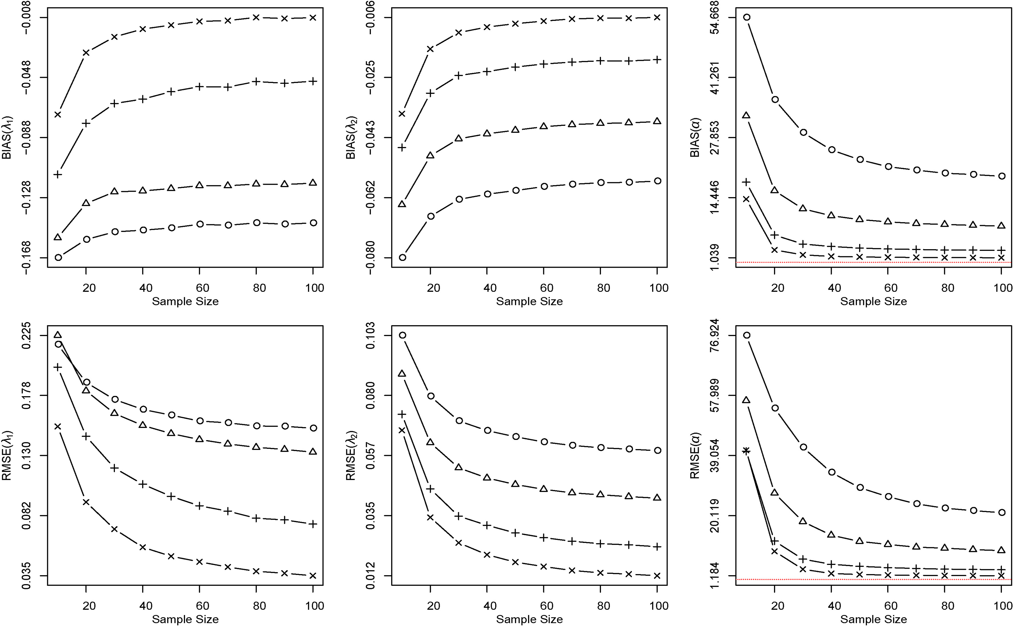
where 10,000 is the number of simulations and denotes each parameter or . The obtained simulation results for each scenario are illustrated, respectively, in Figs 2–4.
The biases (upper panels) and RMSEs (lower panels) for the BDGR distribution assuming () (, 0.90, 2.00) where 0.40; 0.50; : 0.60; 0.70.
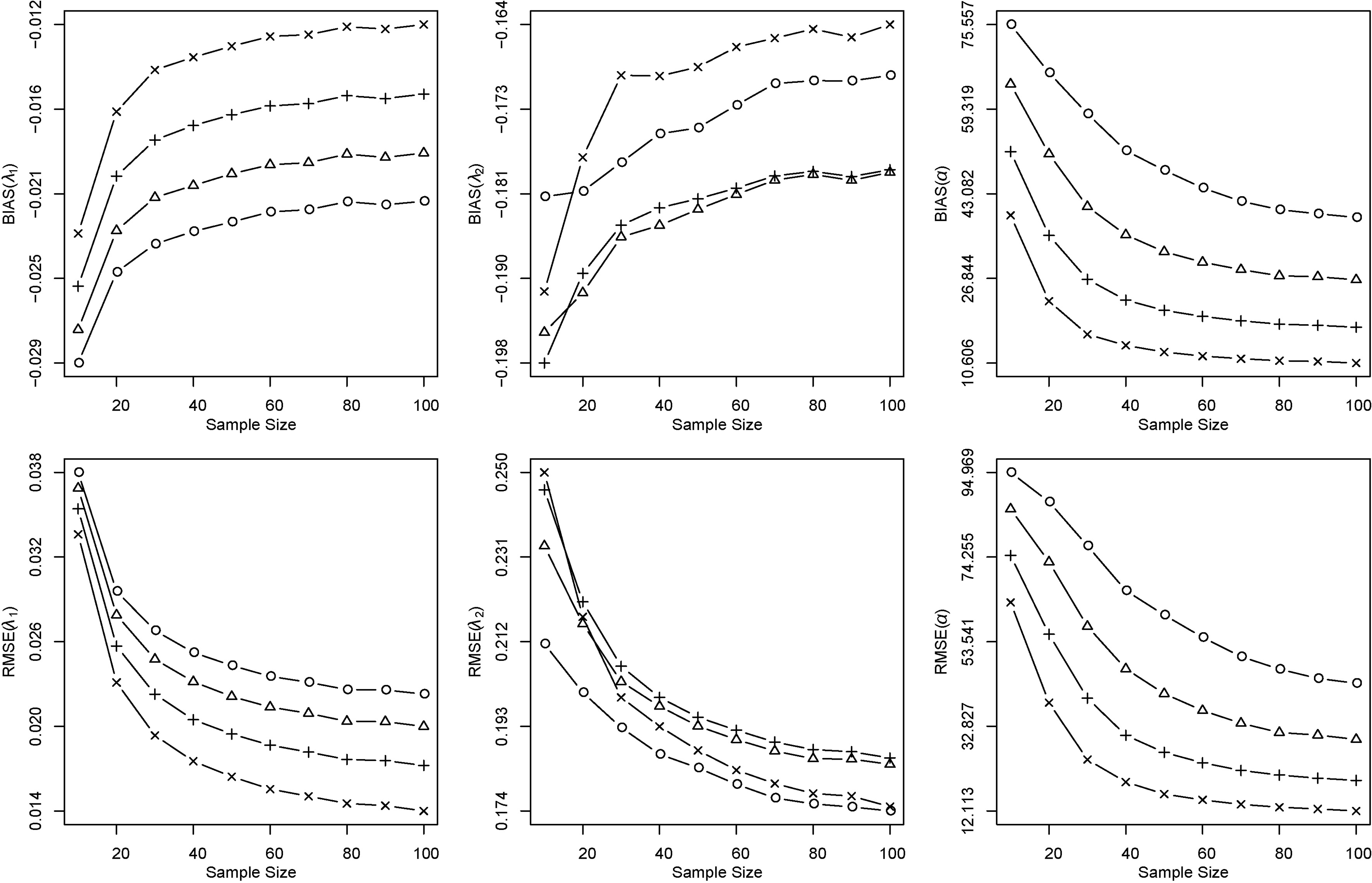
The biases (upper panels) and RMSEs (lower panels) for the BDGR distribution assuming () (0.95, , 2.50) where 0.35; 0.40; : 0.45; 0.50.
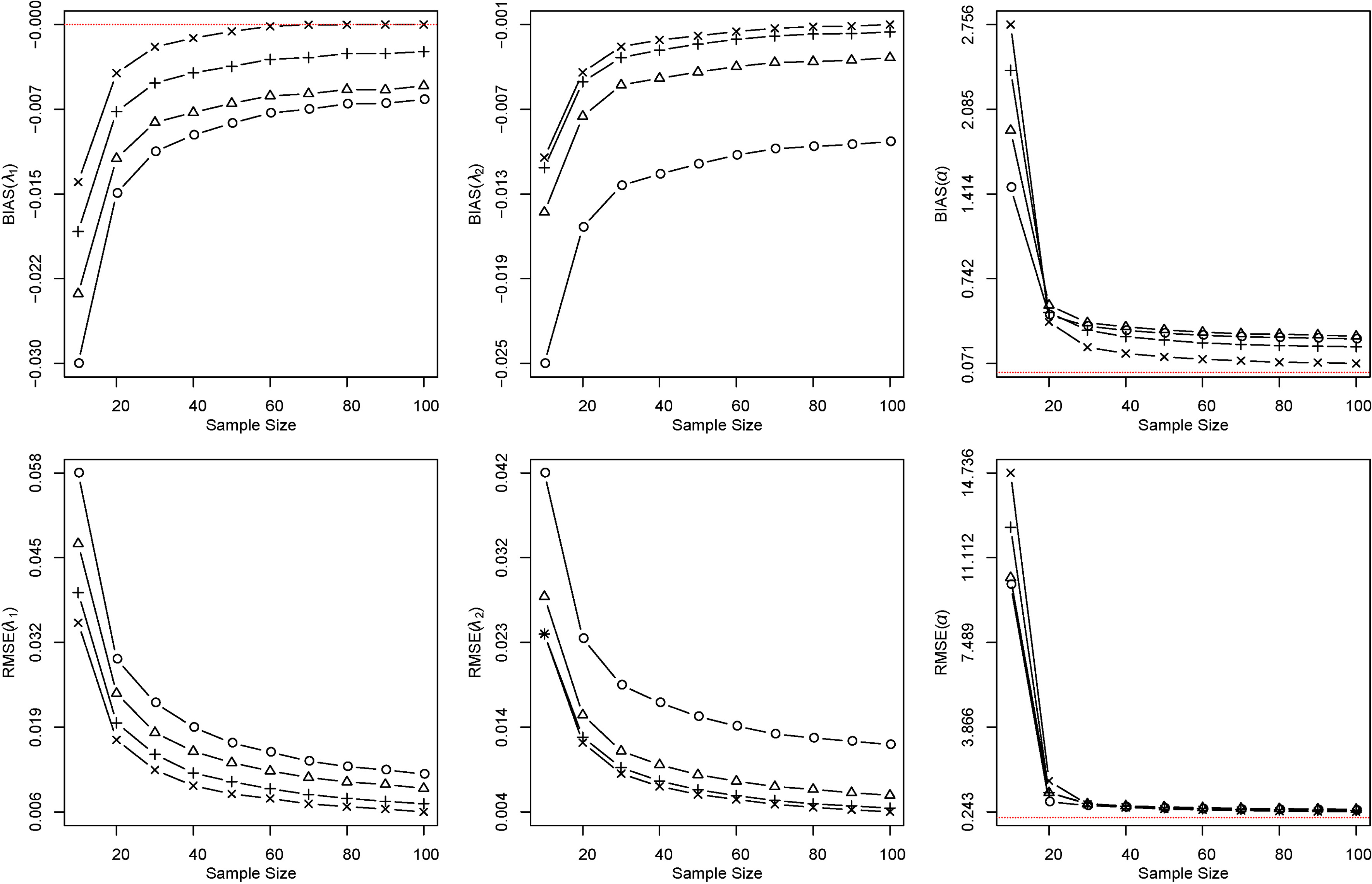
From the simulation results illustrated in Figs 2–4, it is possible to conclude that,
For all considered scenarios, the optimization method converged successful in the determination of the MLEs estimates with no instability for the determination of the biases and RMSEs for all parameters;
For all considered scenarios, the biases and RMSEs tends to zero when the sample size increases. The convergence to zero is much faster in the third scenario ( fixed);
The parameters and have negative biases for all considered scenarios. The parameter has a positive bias for all scenarios;
The parameters and have small values for the biases and RMSEs; however the parameter has high values for the biases and RMSEs;
The smallest values for the biases were obtained for the third scenario; the smallest values for the RMSE were also obtained for the third scenario;
From the simulation results, we concluded that the BDGR distribution has better asymptotically non-biased estimation in the third scenario since 1, 2 and in this scenario; for the other scenarios, we need a sample size n larger than 100 to get the results and ;
It is important to point out that the simulation study also could be made using a Bayesian approach assuming different prior distributions for the parameters of the BDGR distribution.
Based on the results of these simulation studies we conclude that the BDGR distribution could be used as an alternative to other existing discrete bivariate distributions (such as the Basu-Dhar bivariate geometric distribution introduced by Basu & Dhar, 1995) to describe bivariate lifetimes with good accuracy in applications.
A medical example with censored observations and covariates
To illustrate the usefulness of the proposed methodology, we present in this section, the analysis of a real medical dataset related to lung cancer assuming the bivariate discrete generalized Rayleigh distribution. The dataset is introduced by Ding et al. (2017) and corresponds to the lifetimes of Chinese patients with pathologically confirmed lung cancer who received EGFR, KRAS, and BARF mutation tests at the Thoracic Cancer Institute, Tongji University from January 2012 to April 2016.
For the statistical analysis, we assumed as lifetimes the overall survival times (calculated from the date of lung cancer diagnosis to death from any reason or censored at the last follow-up date), and the progression-free survival times (the times from the treatment start time until the date of systemic progression or death). The data set consists of 28 patients with not censored observations for the overall survival times and 4 censored observations for the progression-free survival times. The non-parametric estimators for the means obtained from the kaplan and Meier (1958) non-parametric estimators for the survival functions are given, respectively, by 16.57 months for the overall survival time () and 5.71 months for the progression-free survival time (). We also considered in the statistical analysis of the data, a prognostic factor (smoking status) and an oncological factor (cancer stage) as two covariates possibly affecting the survival times of the patients.
A Bayesian analysis not considering the presence covariates
As a first analysis, the presence of the prognostic and oncology factors (smoking status and cancer stage) were not considered. The fit of BDGR distribution was compared to the fit of a Basu-Dhar bivariate geometric distribution (BDBG) (Basu & Dhar, 1995); to the fit of a Arnold bivariate geometric distribution (ABG) (Arnold, 1975); and to the fit of a generalized bivariate geometric distribution (GBG) (Gómez-Déniz et al., 2017).
The parameters of the models were estimated under a Bayesian approach assuming independent prior distributions for the parameters 1, 2, 12 and a gamma prior distribution with hyperparameter values and where 5.0714, 15.3214, 10.2910 and 36.5966 for the parameter , that is, we used empirical Bayesian methods in the elicitation of the prior distribution for the dependence parameter (see Carlin & Louis, 2000). The DIC criteria was considered to discriminate the best model among all proposed models (smaller values indicate better models, see Spiegelhalter et al., 2014). From the obtained results presented in Table 2, we conclude that the BDGR distribution is the best model fitted by the dataset.
Bayesian estimates assuming bivariate discrete models for the lung cancer dataset
Model
Param.
Mean
S.D.
95% Conf. Int.
Model
Param.
Mean
S.D.
95% Cred. Int.
BDGR
0.4309
0.1139
(0.2386, 0.6909)
GBG
0.8805
0.1040
(0.8255, 0.9973)
0.9848
0.0041
(0.9756, 0.9918)
0.8606
0.0289
(0.8417, 0.9134)
0.9978
0.0006
(0.9963, 0.9988)
0.9413
0.0115
(0.9338, 0.9626)
BDBG
0.7982
0.0335
(0.7768, 0.8570)
ABG
0.1897
0.0311
(0.1675, 0.2533)
0.9697
0.0188
(0.9553, 0.9988)
0.0583
0.0114
(0.0506, 0.0817)
0.9692
0.0187
(0.9551, 0.9984)
DIC 313.75; DIC 329.70; DIC 330.20; DIC 354.60.
The biases (upper panels) and RMSEs (lower panels) for the BDGR distribution assuming () (0.95, 0.97, ) where 0.50; 0.75; : 1.00; 1.25.
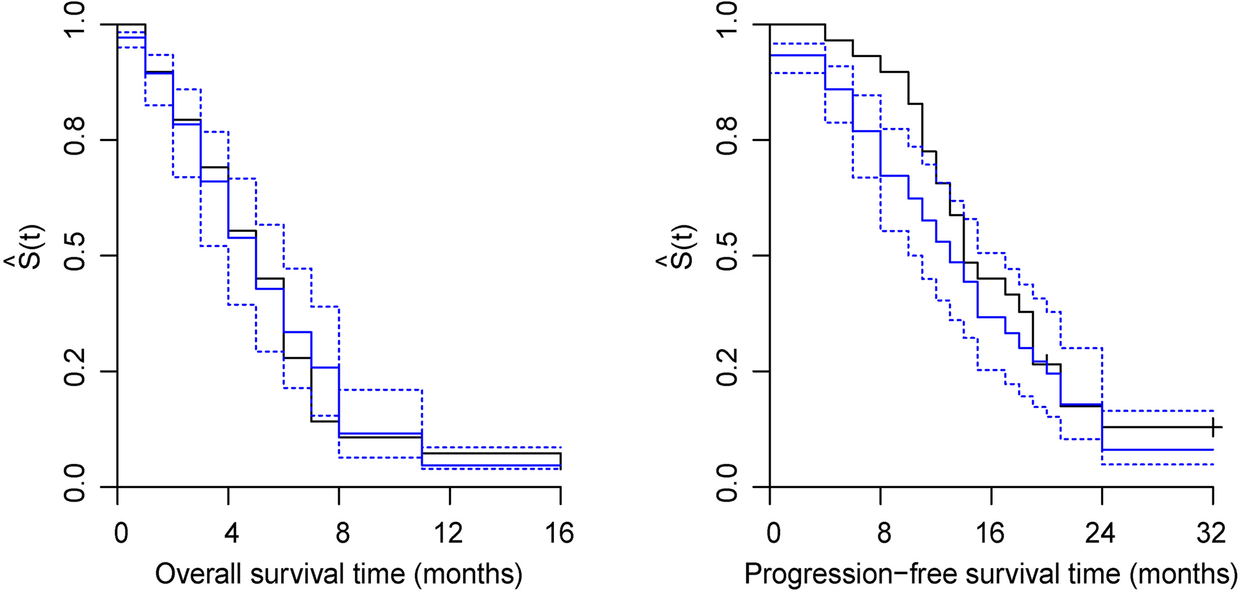
Figure 5 presents the Kaplan-Meier marginal survival plots for both lifetimes and also the estimated survival BDGR functions since this model was verified to be the best fitted model for the dataset. From the graphs of Fig. 5, we conclude that the proposed model has a good accuracy to predict both survival times.
The suitability of the BDGR distribution can also be verified from the marginal distributions which must also be generalized Rayleigh distributions (see Balakrishnan & Ristić, 2016; Ristić et al., 2018). In our application, this is observed from graphs of the Kaplan and Meier non-parametric estimators of the survival functions and the Bayesian estimators of the marginal generalized Rayleigh survival functions for both lifetime times.
In addition, the estimator of the correlation coefficient for the proposed model was compared to the empirical correlation coefficient obtained using the Iterative Multiple Imputation (IMI) method (for more details, see Schemper et al., 2013) available in the package SurvCorr from R software. The empirical correlation coefficient was computed using the function survcorr setting the argument MCMCSteps 210,000. Assuming the BDGR under a Bayesian approach, the Monte Carlo estimator for the correlation coefficient based on the simulated Gibbs samples is given by 0.8726 which is very close to the IMI correlation coefficient given by 0.9328, that is, the proposed model have a good accurate inference result for the correlation coefficient even it is based on a infinite series.
A Bayesian analysis in the presence of the covariates
In the statistical analysis in presence of the prognostic and oncology factors assuming the BDGR distribution, we assumed logistic regression models for the parameters and given by,
where 1, , 28; ; 0 (never-smoker) and 1 (former/current smoker); 0 (stage at diagnosis IIIB) and 1 (stage at diagnosis IV). For a Bayesian analysis of this regression model we assumed normal prior distributions for the regression parameters with zero mean and large variance (approximately non-informative priors) and the same gamma prior distribution considered in Section 5.1 for the parameter . The inference results are reported in Table 3.
Maximum likelihood and Bayesian estimates in presence of prognostic and oncology factors for the lung cancer data set
Param.
Classical approach
Bayesian approach
MLE
S.E.
95% Conf. Int.
Mean
S.D.
95% Cred. Int.
0.6758
0.3063
(0.0755, 1.2761)
0.4342
0.1195
(0.2285, 0.6971)
2.0580
0.7146
(0.6575, 3.4585)
0.1184
1.7907
(3.7383, 3.4465)
1.6732
0.5933
(0.5104, 2.8360)
1.6135
0.6642
(0.3050, 2.9042)
0.8725
0.5111
(0.1291, 1.8742)
0.9004
0.5579
(0.1979, 2.0299)
4.8502
0.6927
(3.4924, 6.2080)
3.8752
1.6987
(0.4833, 7.1144)
0.9195
0.5638
(0.1856, 2.0247)
0.8446
0.6434
(0.4747, 2.1223)
0.4400
0.4753
(0.4917, 1.3716)
0.4860
0.5083
(0.4628, 1.4760)
Criteria
AIC 314.20
DIC 313.18
Kaplan-Meier estimators versus Bayesian estimated survival functions (including the 95% credible interval) for the marginal survival functions and (blue line: fitted model; black line: Kaplan-Meier).
From the results of Table 3, we observed that the Bayesian estimates are very close to the MLEs. Furthermore, we concluded that only the covariate smoker has significant effect on the overall survival time, since the 95% confidence and credible intervals for the regression parameter does not contain the zero value. From the results of Table 3 it is also observed that the parameter has very different classical and Bayesian inference results possible due to the effect of a very non-informative prior for this regression parameter (large 95% credible interval for the parameter). Under the classical approach the obtained inference is obtained under asymptotical results, although there is a small sample size (inference possible not very accurate).
Concluding remarks
The use of existing bivariate discrete distributions could be a good alternative to analyze bivariate lifetime data in presence of censored data and covariates. However, there are few discrete bivariate lifetime distributions introduced in the literature. In general, bivariate lifetime datasets usually are analyzed using standard continuous bivariate lifetime distributions as the popular Block and Basu bivariate exponential distribution (see Block & Basu, 1974) or the Marshall-Olkin bivariate exponential distribution (see Marshall & Olkin, 1967a, 1967b).
In this study, we introduced a new bivariate distribution, denoted as bivariate discrete generalized Rayleigh (BDGR) distribution, obtained using the Marshall and Olkin (1997) method to add a new parameter to the survival function of the discrete Rayleigh distribution proposed by Roy (2004) in order to propose a more flexible joint survival function as an alternative to existing discrete models as the popular Arnold (see Arnold, 1975) and Basu-Dhar (see Basu & Dhar, 1995) bivariate geometric distributions to analyze bivariate discrete lifetime data in presence of censored data and covariates. Some properties of this new distribution were also discussed in this study and an extension to multivariate case was provided.
An extensive simulation study was performed to verify the effectiveness of the maximum likelihood method assuming different fixed values for the parameters of the model and different sample sizes. The results obtained from Monte Carlo studies showed that the biases and RMSEs of the BDGR distribution are asymptotically non-biased and tends to zero when the sample size increases even assuming negative values for 1, 2 in some scenarios.
In the application with real lifetime data presented in this study, we observed that, with the use of the BDGR distribution, it is possible to obtain in a simple way the inferences of interest for bivariate lifetime datasets in presence or not of covariates and censored data with small computational costs as compared to many existing bivariate parametric lifetime distributions introduced in the literature or bivariate models derived from copula functions for continuous bivariate lifetime data (see, for example, Achcar et al., 2016). The identification of important covariates was also easily obtained assuming the BDGR distribution even using non-informative priors for the parameters of the model, under a Bayesian approach. These results could be of great interest for the search of appropriate bivariate lifetime distributions especially in engineering, medical studies or other areas of interest.
Footnotes
Acknowledgments
The authors are grateful to the referees for their valuable suggestions that significantly improved the manuscript.
References
1.
AchcarJ. A., & LeandroR. A. (1998). Use of Markov Chain Monte Carlo methods in a bayesian analysis of the block and basu bivariate exponential distribution.Annals of the Institute of Statistical Mathematics, 50(3), 403-416.
2.
AchcarJ. A.MartinezE. Z., & CuevasJ. R. T. (2016). Bivariate lifetime modeling using copula functions in presence of mixture and non-mixture cure fraction models, censored data and covariates.Model Assisted Statistics and Applications, 11(4), 261-276.
3.
ArnoldB. C. (1975). A characterization of the exponential distribution by multivariate geometric compounding.Sankhyā: The Indian Journal of Statistics, Series A, pp. 164-173.
4.
ArnoldB. C., & StraussD. (1988). Bivariate distributions with exponential conditionals.Journal of the American Statistical Association, 83(402), 522-527.
5.
BalakrishnanN., & LaiC. (2009). Continuous Bivariate Distributions. Springer, New York.
6.
BalakrishnanN., & RistićM. M. (2016). Multivariate families of gamma-generated distributions with finite or infinite support above or below the diagonal.Journal of Multivariate Analysis, 143, 194-207.
BlockH. W., & BasuA. (1974). A continuous, bivariate exponential extension. Journal of the American Statistical Association, 69(348), 1031-1037.
9.
CarlinB. P., & LouisT. A. (2000). Empirical Bayes: Past, present and future. Journal of the American Statistical Association, 95(452), 1286-1289.
10.
ChibS., & GreenbergE. (1995). Understanding the Metropolis-Hastings algorithm. The american statistician, 49(4), 327-335.
11.
DingX.ZhangZ.JiangT.LiX.ZhaoC.SuB., & ZhouC. (2017). Clinicopathologic characteristics and outcomes of Chinese patients with non-small-cell lung cancer and BRAF mutation.Cancer Medicine, 6(3), 555-562.
12.
DowntonF. (1970). Bivariate exponential distributions in reliability theory.Journal of the Royal Statistical Society. Series B (Methodological), pp. 408-417.
13.
FreundJ. E. (1961). A bivariate extension of the exponential distribution. Journal of the American Statistical Association, 56(296), 971-977.
14.
GelfandA. E., & SmithA. F. (1990). Sampling-based approaches to calculating marginal densities. Journal of the American statistical association, 85(410), 398-409.
15.
Gómez-DénizE.GhitanyM., & GuptaR. C. (2017). A bivariate generalized geometric distribution with applications. Communications in Statistics-Theory and Methods, 46(11), 5453-5465.
16.
Gumbel, E. J. (1960). Bivariate exponential distributions. Journal of the American Statistical Association, 55(292), 698-707.
17.
HanagalD., & AhmadiK. (2008). Estimation of parameters by EM algorithm in bivariate exponential distribution based on censored samples. Econ. Quality Control, 23(2), 257-66.
18.
HanagalD. D. (2006). Bivariate Weibull regression model based on censored samples. Statistical Papers, 47(1), 137-147.
19.
HawkesA. G. (1972). A bivariate exponential distribution with applications to reliability. Journal of the Royal Statistical Society. Series B (Methodological), pp. 129-131.
20.
HougaardP. (1986). A class of multivariate failure time distributions. Biometrika, pp. 671-678.
KaplanE. L., & MeierP. (1958). Nonparametric estimation from incomplete observations. Journal of the American statistical association, 53(282), 457-481.
23.
KempA. W. (2013). New discrete appell and humbert distributions with relevance to bivariate accident data. Journal of Multivariate Analysis, 113, 2-6. Kemp and Papageorgiou, 1982 Kemp, C., & Papageorgiou, H. (1982). Bivariate Hermite distributions. Sankhyā: The Indian Journal of Statistics, Series A, pp. 269-280. Kocherlakota, 1995 Kocherlakota, S. (1995). Discrete bivariate weighted distributions under multiplicative weight function. Communications in statistics-theory and methods, 24(2), 533-551. Kocherlakota and Kocherlakota, 1992 Kocherlakota, S., & Kocherlakota, K. (1992).Bivariate discrete distributions. Wiley Online Library.
24.
KumarC. S. (2008). A unified approach to bivariate discrete distributions. Metrika, 67(1), 113-123.
25.
Kundu,D. (2014). Geometric skew normal distribution. Sankhya B, 76(2), 167-189.
KunduD.BalakrishnanN., & JamalizadehA. (2010). Bivariate birnbaum–saunders distribution and associated inference. Journal of Multivariate Analysis, 101(1), 113-125.
28.
KunduD., & GuptaR. D. (2009). Bivariate generalized exponential distribution. Journal of Multivariate Analysis, 100(4), 581-593.
29.
KunduD., & NekoukhouV. (2018). Univariate and bivariate geometric discrete generalized exponential distributions. Journal of Statistical Theory and Practice, 12(3), 595-614.
30.
LaiC.-D. (2006). Constructions of discrete bivariate distributions. In Advances in Distribution Theory, Order Statistics, and Inference, pp. 29-58. Springer.
31.
LawlessJ. F. (1982). Statistical models and methods for lifetime data. John Wiley & Sons.
32.
LeeH., & ChaJ. H. (2014). On construction of general classes of bivariate distributions. Journal of Multivariate Analysis, 127, 151-159.
33.
MarshallA. W., & OlkinI. (1967a). A generalized bivariate exponential distribution. Journal of Applied Probability, 4(2), 291-302.
34.
MarshallA. W., & OlkinI. (1967b). A multivariate exponential distribution. Journal of the American Statistical Association, 62(317), 30-44.
35.
MarshallA. W., & OlkinI. (1997). A new method for adding a parameter to a family of distributions with application to the exponential and Weibull families. Biometrika, 84(3), 641-652.
36.
MirMostafaeeS.MahdizadehM., & LemonteA. J. (2017). The Marshall – Olkin extended generalized Rayleigh distribution: Properties and applications.Communications in Statistics-Theory and Methods, 46(2), 653-671.
PopovićB. V., & GençA. İ. (2018). On extremes of two-dimensional Student-t distribution of the Marshall–Olkin type.Mediterranean Journal of Mathematics, 15(4), 153.
39.
R Core Team (2016). R: A Language and Environment for Statistical Computing. R Foundation for Statistical Computing, Vienna, Austria.
RoyD. (2004). Discrete Rayleigh distribution.IEEE Transactions on Reliability, 53(2), 255-260.
42.
SarkarS. K. (1987). A continuous bivariate exponential distribution. Journal of the American Statistical Association, 82(398), 667-675.
43.
SchemperM.KaiderA.WakounigS., & HeinzeG. (2013). Estimating the correlation of bivariate failure times under censoring.Statistics in medicine, 32(27), 4781-4790.
44.
SpiegelhalterD. J.BestN. G.CarlinB. P., & Van Der LindeA. (2014). The deviance information criterion: 12 years on. Journal of the Royal Statistical Society: Series B (Statistical Methodology), 76(3), 485-493.
45.
SuY.-S., & YajimaM. (2012). R2jags: A package for running jags from r. R package version 0.03-08, URL http://CRAN. R-project. org/package= R2jags.