Bayesian analysis of Birnbaum-Saunders survival model with cure fraction under a variety of activation mechanism

Abstract

In this paper we propose a new cure rate survival model. Our approach enables different underlying activation mechanisms which lead to the event of interest. The number of competing causes which may be responsible for the occurrence of the event of interest is assumed to follow a geometric distribution while the time to event is assumed to follow a Birnbaum-Saunders distribution. As an advantage our approach may scan all underlying activation mechanisms from the first to last one based on order statistics. We explore the use of Markov chain Monte Carlo methods to develop a Bayesian analysis for the proposed model. Moreover, some discussions on the model selection to compare the fitted models are given. In particular, case deletion influence diagnostics are developed for the joint posterior distribution based on the $\psi$ -divergence, which includes the Kullback-Leibler (K-L), $J$ -distance, $L_{1}$ norm and $\chi^{2}$ -square divergence measures as particular cases. Simulation studies are performed for study frequentist properties of the Bayesian estimates. The methodology is illustrated on a real malignant melanoma data.

Keywords

Birnbaum-Saunders distribution Cure fraction models Geometric distribution o lifetime data sensitivity analysis

1. Introduction

In many medical problems, such as chronic cardiac diseases and various different types of cancer, a cumulative individual damage may be caused by various unknown causes or risk factors. This degradation leads to a fatigue process, whose propagation lifetimes can be suitably modeled by a Birnbaum-Saunders (BS) distribution. The BS distribution was originated from a physical problem related to material fatigue, describing the total time that passes until the development and growth of a dominant crack, producing a type of cumulative damage that surpasses a threshold and causes a failure (Birnbaum & Saunders, 1969). Leiva et al. (2007) applied the classical version of the BS distribution (BS model generated from the normal law) for modeling lifetimes of patients with multiple myeloma.

A review of all developments on BS distribution and related distributions can be found in Balakrishnan and Kundu (2019).

The survival function of BS model is given by

$\displaystyle S_{\textit{BS}}(t)=\Phi\left[-\frac{1}{\alpha}\left(\sqrt{\frac{% t}{\lambda}}-\sqrt{\frac{\lambda}{t}}\right)\right],\;t>0,$ (1)

where $\Phi(.)$ is the standard normal cumulative distribution function, $\alpha>0$ and $\lambda>0$ are respectively, shape and scale parameters. The corresponding probability density function (pdf) of the BS distribution is obtained from Eq. (1) as

$\displaystyle f_{\textit{BS}}(t)=\frac{t^{-3/2}\,(t+\lambda)}{2\alpha\,\sqrt{2% \pi\lambda}}\,\,\exp\left[-\frac{1}{2\alpha^{2}}\left(\frac{t}{\lambda}+\frac{% \lambda}{t}-2\right)\right].$ (2)

The parameter $\lambda$ is the median of the distribution: $F_{\textit{BS}}(\lambda)=1-S_{\textit{BS}}(\lambda)=\Phi(0)=1/2$ . The mean and the variance of the BS distribution are respectively $\text{E}(T)=\lambda\,(1+({\alpha^{2}}/{2}))$ and $\text{Var}(T)=\alpha^{2}\,\lambda^{2}\,(({5}/{4})\alpha^{2}+1).$

Some proposals have been made in the literature by replacing the relationship between the BS and normal distributions by more general classes of distributions. For example, Díaz-García and Leiva-Sánchez (2005) introduce the generalized BS distribution by considering the elliptical family of distributions. The main motivation for considering the generalized BS distribution is to make the kurtosis flexible compared to the BS model. Sanhueza et al. (2008) presented a complete compilation of the results related to the generalized BS distribution and Gómez et al. (2009) proposed an extension of the generalized BS model based on the slash-elliptical distributions.

Moreover, from the practical point of view, due to significant progress and advancements in treatment therapies, it is common that we observe survival data where part of the population is not susceptible to the event of interest. For instance, in clinical studies a population can respond favorably to a treatment, being considered cured. The proportion of such fraction of the population which is not susceptible to the event of interest is usually termed as the cured fraction. In this context, in order to address such conceptual problem, cure rate models (also called survival models with a surviving fraction or long-term survival models) that incorporate a cure fraction have been proposed and are nowadays widely developed. Perhaps the most popular type of cure rate model is the mixture distribution introduced by Boag (1949) and Berkson and Gage (1952), where it is assumed that a certain proportion of the patients are cured, in the sense that they do not present the event of interest during a long period of time and can be seen as to be immune or cured to the cause of death under study. A key reference on mixture distributions is Maller and Zhou (1996).

Mixture models are based on the assumption that only a cause is responsible for the occurrence of the event of interest. However, in clinical studies, the patient’s death or recurrence of tumor, which is the event of interest, may happen due to different latent competing causes, in the sense that there is no information about which cause was responsible for disease manifestation through the occurrence of the event of interest. A tumor recurrence can be attributed to metastasis-component tumor cells left active after initial treatment. A metastasis-component tumor cell is a tumor cell with potential to metastasize (Yakovlev & Tsodikov, 1996). In the above context, the literature on distributions which accommodates different latent competing causes is rich and growing rapidly. The book by Ibrahim et al. (2001), the review paper by Tsodikov et al. (2003) and the works by Cooner et al. (2007), Rodrigues et al. (2009), Cancho et al. (2009) and Cancho et al. (2012a) can be regarded as key references. Another approach, by Cooner et al. (2006) and Cooner et al. (2007), forms an arranged stochastic sequence of latent causes, which induce the occurrence of the event of interest via an underlying activation mechanisms that lead to the event of interest. The cure rate models have been successfully applied to many real word problems. For example, Cancho et al. (2013), Suzuki et al. (2016) and Suzuki et al. (2017) assumed that unobservable number of causes of an event of interest follows the Negative Binomial, Poisson and Logarithmic distributions, respectively.

The main goal of this paper is to present a new distribution family, hereafter called the GBS cure rate (GBScr) model, conceived inside a scenario of latent competing causes with the presence of a cure fraction, where the occurrence of the event of interest may be activated by different kinds of mechanisms (Cooner et al., 2007).

The GBScr model includes a particular case of the model introduced by Cancho et al. (2012b) in presence of a first activation mechanism.

Bayesian analysis for the BS model has appeared in the literature. For instance we cite Tsionas (2001) and Xu and Tang (2011). In this paper, we propose a Bayesian approach for drawing inferences in GBScr models in the presence of covariates on the cure fraction. Also, we develop case deletion influence diagnostics for the joint posterior distributions of the parameters of the GBScr model based on the $\psi$ -divergence measure (Peng & Dey, 1995; Weiss, 1996). The $\psi$ -divergence measure includes several divergence measures as particular cases, such as the Kullback-Leibler (K–L), $J$ -distance, $L_{1}$ norm and $\chi^{2}$ -square divergence measures.

The paper is organized as follows. In Section 2 we formulate the model, providing its particular cases as well as a comparison among the activation mechanisms. The development of a Bayesian analysis is presented in Section 3, involving inference, Model comparison and case influence diagnostics. A simulation study with the different models is presented in Section 4, where we discuss the results of the evaluation of the frequentist properties as well as the influence of outlying observations. An application to a real data set is developed in Section 5. Finally, Section 6 ends up the paper with some general remarks.

2. Model formulation

The GBScr distribution is derived as follows. For an individual in the population, let $M$ denote the unobservable number of causes of the event of interest for this individual. Assume that $M$ follows a geometric distribution with parameter $\theta$ and probability mass function,

$\displaystyle P(M=m)=\theta(1-\theta)^{m},\;\;m=0,1,\ldots.$ (3)

The time for the $j^{\text{th}}$ cause to produce the event of interest is denoted by $Z_{j}$ , $j=1,\ldots,M$ . We assume that, conditional on $M$ , the $Z_{j}$ are independent identically distributed accordion to a BS distribution given in Eq. (1). Also, we assume that $Z_{1}$ , $Z_{2},\ldots$ are independent of $M$ . The observable time to event is defined by the random variable $Y=Z_{(R)}$ , where $R$ depends on $M$ , $Z_{(1)}\leqslant Z_{(2)}\leqslant\ldots\leqslant Z_{(R)}\leqslant\ldots% \leqslant Z_{(M)}$ are the order statistics and $Y=\infty$ if $M=0$ . In many biological processes $R$ can be interpreted as a resistance factor of the immune system of the individual. If the event of interest occurs (e.g., cancer relapse), then the random variable $Y$ takes the value of the $R^{\text{th}}$ order statistics $Z_{(R)}$ . In other words, as in Cooner et al. (2006) and Cooner et al. (2007), $R$ out of $M$ causes are required to produce the event of interest. Moreover, the activation mechanism may be seem as a system of hits generated by independent times to hit $Y$ , where $R$ is the number of hits required to make the system fail. The resistance factor can be a fixed constant, a function of $M$ or a random variable specified through a conditional distribution on $M$ .

In this paper, using the terminology borrowed from Cooner et al. (2006) and Cooner et al. (2007), we deal with three specifications for $R$ , $R=1$ directing to a first activation mechanism, random $R$ directing to a random activation mechanism and $R=M$ directing to a last activation mechanism. Thus we scan all possible mechanisms of activation.

Although, one may have information beforehand about activation mechanism which should be considered for a particular application. For example, focusing in reliability, if a series system is considered to be analyzed than the first activation mechanism is the natural one, while the last activation mechanism is the natural one in presence of a parallel system. However, as in many situations we may have difficulties to view, in a simplistic way, which activation mechanism is the most adequate, our approach is, at least in principle, more intuitive, with ability to scan all the possibilities between the first and the last activation mechanisms. For instance, focusing in the medical area, it may be difficult to decide for a particular activation mechanism acting on the occurrence of a disease. Although a tumor recurrence can be attributed to metastasis-component tumor cells left active after initial treatment, which activation mechanism may represent the phenomenon? In this context, the GBScr with a scan type activation mechanism may be considered as its different particular cases. We then may decide for the best fitting in the light of the dataset via a model comparison criteria as it will be pointed out further in the text.

2.1 Activation mechanisms

We first assume that given $M\geqslant 1$ , the conditional distribution of $R$ is uniform on $\{1,\ldots,M\}$ (a random activation mechanism). Under this setup, the surviving function for the population is given by

$\displaystyle S_{\text{GBScr}}(y)=P(Y>y)=P(M=0)+\sum_{k=1}^{\infty}\sum_{R=1}^% {k}P(Z_{(R)}>y|R,M=k)P(R|M=k)P(M=k),$ (4)

where

$\displaystyle P(Z_{(R)}>y|R,M=k)=\sum_{i=0}^{R-1}{k\choose i}(F_{\textit{BS}}(% y))^{i}(S_{\textit{BS}}(y))^{k-i}.$ (5)

Note that Eq. (5) gives the cumulative distribution function (cdf) of binomial distribution, with $k$ trials and success probability $F_{\textit{BS}}(y)$ . If R=1, then, $P(Z_{(1)}>y|R,M=k)=S_{\textit{BS}}(y)^{k}$ , which includes the models proposed by Tsodikov et al. (2003).

From Eq. (5), the survival function of $Y$ in Eq. (4) under random activation mechanism is given by

$\displaystyle S_{\text{GBScr}}(y)=P(M=0)+\sum_{k=1}^{\infty}\left\{\sum_{R=0}^% {k}(k-R)B(R;k,F_{\textit{BS}}(y))\right\}\frac{1}{k}\theta(1-\theta)^{k}=P(M=0% )+S_{\textit{BS}}(y)\sum_{k=1}^{\infty}\theta(1-\theta)^{k}=\theta+(1-\theta)S% _{\textit{BS}}(y),$ (6)

where $B(x;k,F_{\textit{BS}}(y))=P(X=x)$ and $X\sim\textit{Binomial}(k,F(y))$ . We observe that the $S_{\text{pop}}(y)$ in Eq. (6) is a mixture cure model with cured fraction $p_{0}=P(M=0)=\lim_{y\to\infty}S_{\text{pop}}(y)=\theta$ . From Eq. (6), the density function is $f_{\text{GBScr}}(y)=-S_{\text{GBScr}}^{\prime}(y)=(1-\theta)f_{\textit{BS}}(y).$ Furthermore, the corresponding hazard function is $h_{\text{GBScr}}(y)={(1-\theta)f_{\textit{BS}}(y)}/\{\theta+(1-\theta)S_{BS}(y)\}$ .

As a second setup, the so-called first activation mechanism, we suppose that the event of interest happens due to the possible cause with firstly happened. Therefore, for $R=1$ , the time to event is $Y=Z_{(1)}=\min\{Z_{1},\ldots,Z_{M}\}$ . From Eqs (4) and (5), the survival function of $Y$ is given by

$\displaystyle S_{\text{GBScr}}(y)=P(M=0)+\sum_{k=1}^{\infty}S_{\textit{BS}}(y)% ^{k}P(M=k)=\theta+\theta\sum_{k=1}^{\infty}\left[S_{\textit{BS}}(y)(1-\theta)% \right]^{k}=\frac{\theta}{1-(1-\theta)S_{\textit{BS}}(y)}.$ (7)

The cured fraction is given by $p_{0}=\theta$ . The density function associated to Eq. (7) is given by $f_{\text{GBScr}}(y)={\theta(1-\theta)f_{\textit{BS}}(y)}{[1-(1-\theta)S_{% \textit{BS}}(y)]^{-2}},$ with hazard function $h_{\text{GBScr}}(y)={(1-\theta)f_{\textit{BS}}(y)}$ ${[1-(1-\theta)S_{\textit{BS}}(y)]^{-1}}$ . Note that the model Eq. (7) corresponding the model proposed by Cancho et al. (2012b).

In our third scenario, also known as the last activation mechanism, the event of interest only takes place after all the $M$ causes have been occurred, so that $R=M$ and the observed failure time is $Y=Z_{(M)}=\max\{Z_{1},\ldots,Z_{M}\}$ . From Eqs (4) and (5), we have that survival function of $Y$ is given by

$\displaystyle S_{\text{GBScr}}(y)=P(M=0)+\sum_{k=1}^{\infty}[1-F_{\textit{BS}}% (y)^{k}]P(M=k)=1-\theta\sum_{k=1}^{\infty}\left[F_{\textit{BS}}(y)(1-\theta)% \right]^{k}=1+\theta-\frac{\theta}{1-(1-\theta)F_{\textit{BS}}(y)},$ (8)

so that the cured fraction is $p_{0}=\theta$ . The surviving function in Eq. (8) leads to the density function $f_{\text{GBScr}}(y)={\theta(1-\theta)f_{\textit{BS}}(y)}{[1-(1-\theta)F_{% \textit{BS}}(y)]^{-2}},$ with hazard function $h_{\text{GBScr}}(y)={\theta(1-\theta)f_{\textit{BS}}(y)}/\{[1-(1-\theta)F_{% \textit{BS}}(y)]^{2}[1+\theta-\frac{\theta}{1-(1-\theta)F_{\textit{BS}}(y)}]\}$ .

2.2 On the comparison of the activation mechanisms

We note that $f_{\text{GBScr}}(y)$ and $h_{\text{GBScr}}(y)$ are improper functions whichever the activation mechanism, since $S_{\text{GBScr}}(t)$ is not a proper survival function. But, the cured fraction is the same. The models differ by its surviving, density and hazard functions. The relationship between the survival functions in Eqs (4), (7) and (8) is described in next proposition. Figure 1 portrays distinct behaviors of the survival functions (left panel). These plots illustrate the flexibility built on our proposal. Moreover, the following proposition delimits the survival functions related to each activation mechanism presented in this paper.

Figure 1.

Survival functions populational (left panel) and non-cured populational (right panel) for the GBScr models with $\theta=$ 0.3, $\alpha=$ 5 and $\lambda=$ 5.0 under different activations (first: dashed, random: solid and last: dotted).

.

Under conditions of models in Eqs (6)–(8) and for the cdf $F_{\textit{BS}}(y)$ given in Eq. (1), we have that: $S_{\text{GBScr}}(y)$ in Eq. (7) $\leqslant S_{\text{GBScr}}(y)$ in Eq. (6) and $S_{\text{GBScr}}(y)$ in Eq. (8) $\geqslant S_{\text{GBScr}}(y)$ in Eq. (6).

The proof of the Proposition 1 follows immediately from the Theorem 1 from Kim et al. (2011).

The (proper) surviving function for the non-cured population, denoted by $S_{\text{GBS}}$ is computed by $S_{\text{GBS}}(y)=P(Y>y|M\geqslant 1).$ For a random activation mechanism, $S_{\text{GBS}}$ is the same distribution of the latent random variable $Z_{j}$ ’s, that is, $S_{\text{GBS}}(y)=S_{\textit{BS}}(y)$ . For the first activation mechanism, the survival function for the non-cured population is given by

$\displaystyle S_{\text{GBS}}(y)=\frac{\theta\Phi\left[-\frac{1}{\alpha}\left(% \sqrt{\frac{y}{\lambda}}-\sqrt{\frac{\lambda}{y}}\right)\right]}{1-(1-\theta)% \Phi\left[-\frac{1}{\alpha}\left(\sqrt{\frac{y}{\lambda}}-\sqrt{\frac{\lambda}% {y}}\right)\right]}.$ (9)

We note that $S_{\text{GBS}}(0)=1$ and $S_{\text{GBS}}(\infty)=0$ , so that Eq. (9) is proper survival function. This survival function is same as the one given in Cancho et al. (2012b).

The survival function for the non-cured population under the last activation mechanism is given by

$\displaystyle S_{\text{GBS}}(y)=\frac{\Phi\left[-\frac{1}{\alpha}\left(\sqrt{% \frac{y}{\lambda}}-\sqrt{\frac{\lambda}{y}}\right)\right]}{1-(1-\theta)\Phi% \left[\frac{1}{\alpha}\left(\sqrt{\frac{y}{\lambda}}-\sqrt{\frac{\lambda}{y}}% \right)\right]}.$ (10)

We note that $S_{\text{GBS}}(0)=1$ and $S_{\text{GBS}}(\infty)=0$ , so that Eq. (10) is proper survival function. From Proposition 1, we have $S_{\text{GBS}}(y)$ in Eq. (9) $\leqslant$ $S_{\text{GBS}}(y)$ in Eq. (10). This relation also, can be observed in Fig. 1 (right panel). Moreover, as pointed out by the referee, we made looked for different thetas which make equal models under different activation mechanisms. For instance, considering the GBS distribution under the first activation mechanism Eq. (9) with $0<\theta_{1}<1$ and the GBS distribution under the last activation mechanism Eq. (10) with $0<\theta_{1}<1$ . It is easy to show they are equal if $\theta_{2}=1/\theta_{1}$ .

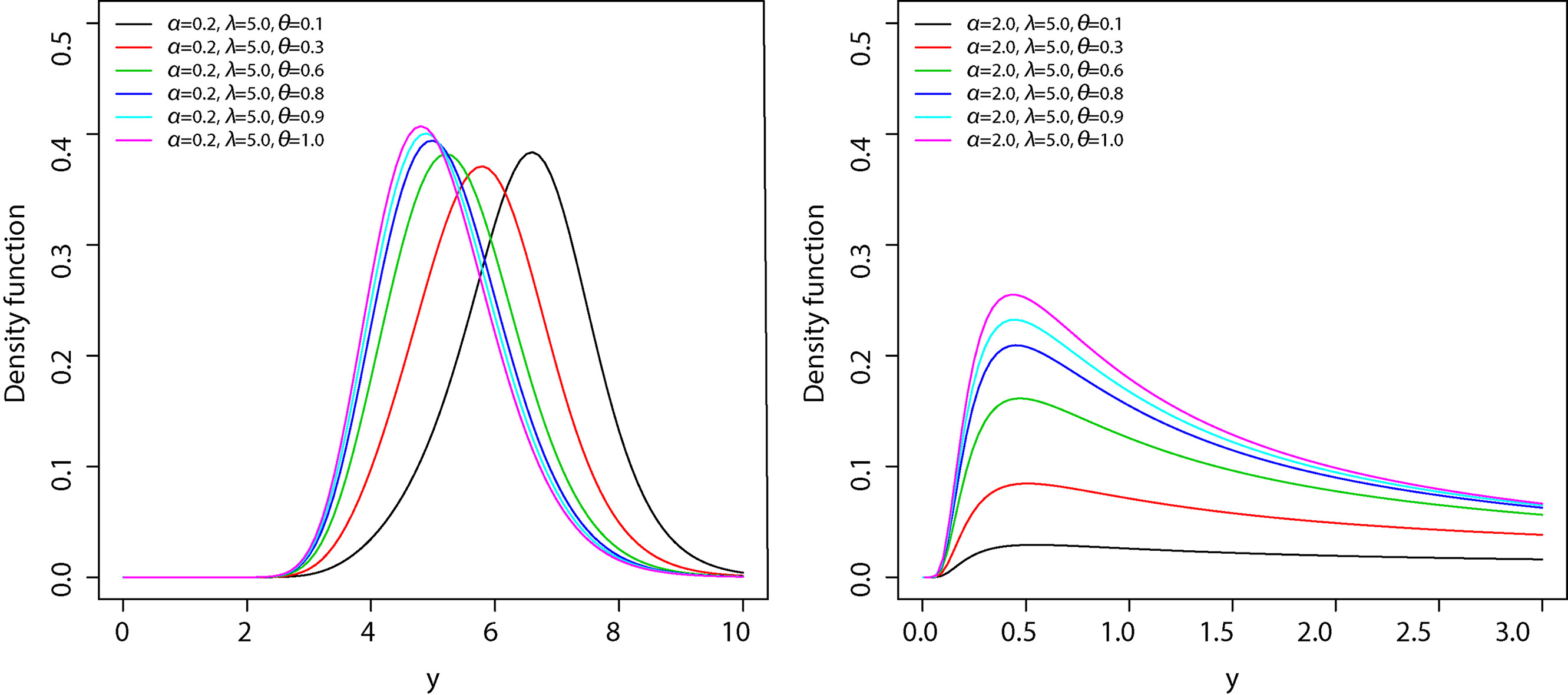
The GBS pdf is given by

$\displaystyle f_{\text{GBS}}(y)=\frac{y^{-3/2}\,(y+\lambda)\theta\exp\left[-% \frac{1}{2\alpha^{2}}\left(\frac{y}{\lambda}+\frac{\lambda}{y}-2\right)\right]% }{2\alpha\,\sqrt{2\pi\lambda}\left\{1-(1-\theta)\Phi\left[\frac{1}{\alpha}% \left(\sqrt{\frac{y}{\lambda}}-\sqrt{\frac{\lambda}{y}}\right)\right]\right\}^% {2}}.$ (11)

In Fig. 2, we plot the GBS last activation density functions for some fixed values of $\alpha$ , $\lambda$ and $\theta$ . These plots indicate that the GBS last activation distribution is very flexible and that the values of $\lambda$ and $\theta$ have a substantial effect on its skewness and kurtosis.

Figure 2.

Probability density function of the GBS distribution under last activation mechanism for some parameter values.

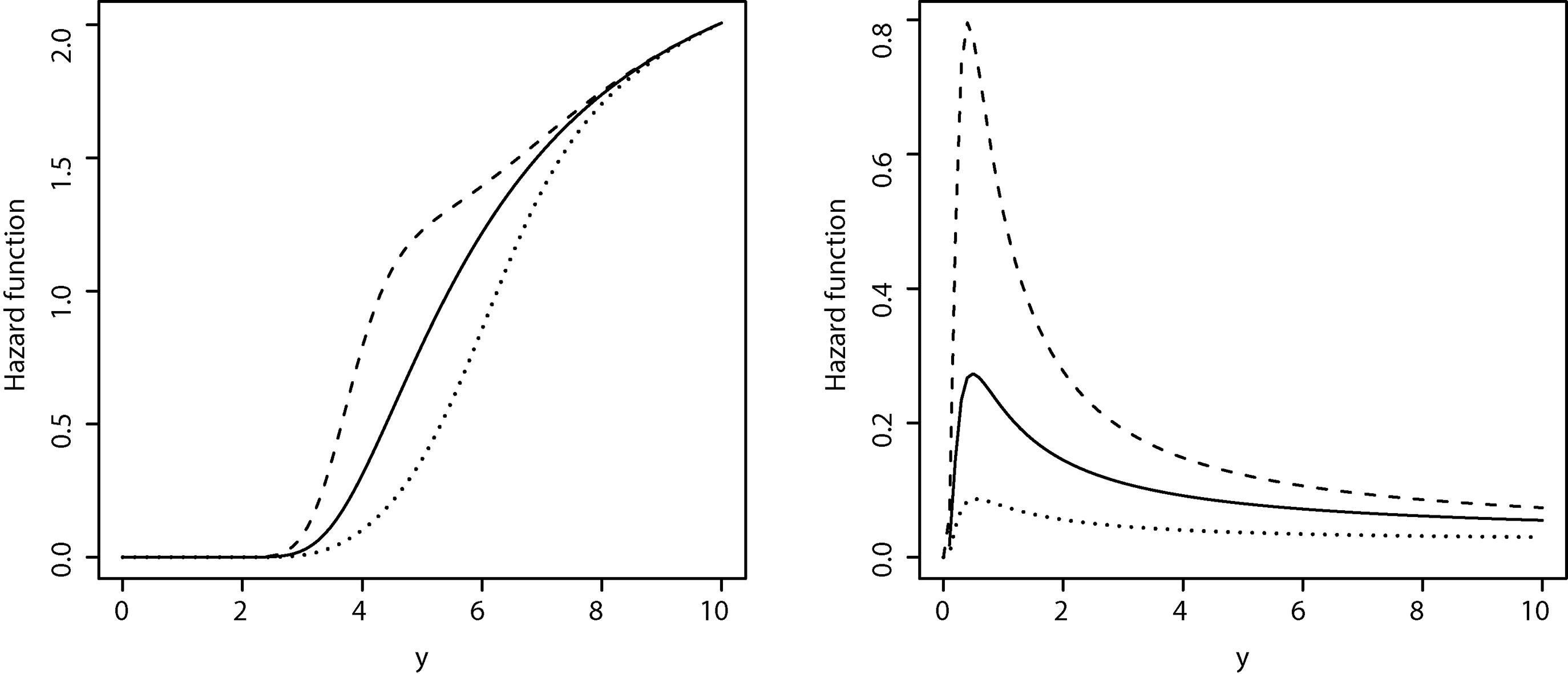
From Eq. (11) and Eq. (10) it is easy to verify that the corresponding GBS hazard function for the population of non-cured is given

$\displaystyle h_{\text{GBS}}(y)=\frac{h_{\textit{BS}}(y)}{1-(1-\theta)F_{% \textit{BS}}(y)},\;\;y>0,$ (12)

where $h_{\textit{BS}}(y)$ and $S_{\textit{BS}}(y)$ are hazard and survival functions of a BS distribution respectively. From Eq. (12), $h_{\text{GBS}}(y)/h_{\textit{BG}}(y)$ is decreasing in $y>0$ for $0<\theta<1$ . Beside, $h_{\textit{BS}}(y)\geqslant h_{\text{GBS}}(y)$ and $\lim_{y\rightarrow\infty}h_{\text{GBS}}(y)=1/2\alpha^{2}\lambda\theta$ and hence we have that the limit behavior of the hazard function of GBS distribution is the same as the behavior of the hazard function of the BS distribution. In the case of first activation mechanism, the limit behavior of the hazard function of the GBS distribution is the reversed of the behavior of the hazard function of the BS distribution. Figure 3 shows some GBS hazard function shapes for some fixed values of parameters.

Figure 3.

Hazard function of the GBS distribution with $\theta=0.3$ , and $\lambda=5.0$ under different activations (first: dashed, random: solid and last: dotted) for $\alpha=0.2$ (left panel) and $\alpha=2.0$ (right panel).

There is a mathematical relationship between the models Eqs (7) and (8) and the mixture cure rate model (Boag, 1949; Berkson & Gage, 1952) We can write

$\displaystyle S_{\text{GBScr}}(y)=\theta+(1-\theta)S_{\text{GBS}}(y),$

where $S_{\text{GBS}}(y)$ is given by Eqs (9) or (10). Thus, $S_{\text{GBScr}}(y)$ is a mixture cure rate model with cure rate equal to $p_{0}=\theta$ and survival function $S_{\text{GBS}}(y)$ for the non-cured population. This results implies that every mixture cure rate model corresponds to some model of the form Eq. (7) (first activation mechanism) or Eq. (8) (last activation mechanism) for any $\theta$ and $S_{\textit{BS}}(\cdot)$ . This result holds for any distribution function.

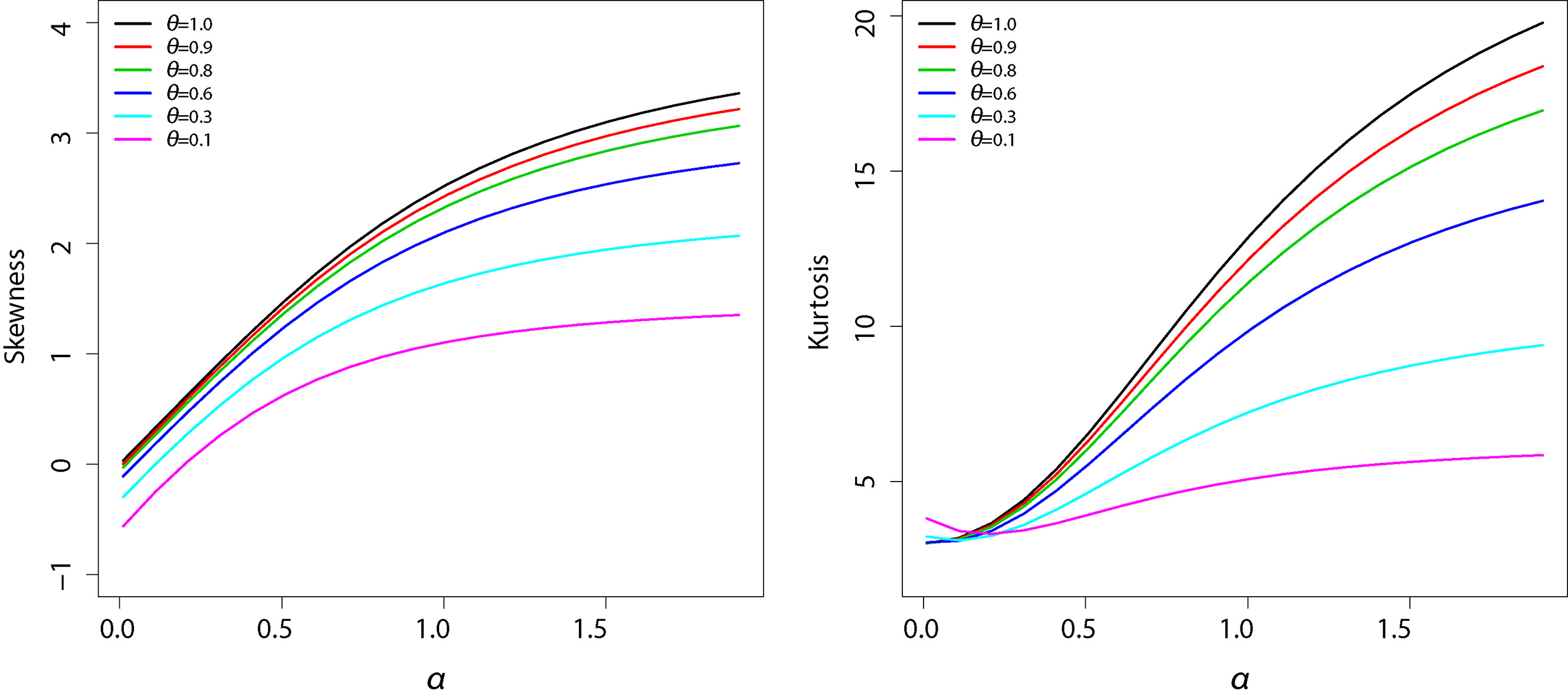
The $r^{th}$ moment of the GBS distribution under the last activation mechanism is given by

$\displaystyle\mu{{}^{\prime}}_{r}=E(Y^{r})=\int_{0}^{\infty}ry^{r-1}S_{\text{% GBS}}(y)dy,$ (13)

where $S_{\text{GBS}}(y)$ is given in Eq. (10). Note that in Eq. (13) for $\theta=1$ , the moments agree with the respective moments of the BS distribution. The skewness and kurtosis measures can be calculated from the ordinary moments given in Eq. (13) using well-known relationships and they can be easily computed numerically in a statistical software such as R (R Development Core Team, 2010). Figure 4 shows a graphical representation of skewness and kurtosis for GBS last activation distribution. It is observed that both skewness and kurtosis are increasing functions of $\alpha$ and $\theta$ . The $r^{th}$ moment of the GBS distribution under the first activation mechanism are calculated in the same manner. The results are similar to the ones obtained for the GBS distribution under the last activation mechanism and are therefore not shown.

Figure 4.

Left panel: Skewness of the GBS distribution under the last activation mechanism. Right panel: Kurtosis of the GBS distribution under the last activation mechanism. The parameters were fixed $\theta=0.1,0.3,0.6,0.8,0.9,1$ and $\lambda=5$ , for $0<\alpha<2$ .

Overall, it seems to be a perfect complementarity between the mechanisms of activation, which can be observed confronting the behavior of the graphs shown in Fig. 1 (survival functions) and 3 (hazard functions).

3. Inference

Let us consider the situation when the failure time $Y$ in Section 2 is not completely observed and is subject to right censoring. Let $C_{i}$ denote the censoring time. In a sample of size $n$ , we then observe $T_{i}=\min\{Y_{i},C_{i}\}$ and $\delta_{i}=\text{I}(Y_{i}\leqslant C_{i})$ , where $\delta_{i}=1$ if $T_{i}$ is a failure time and $\delta_{i}=0$ if it is right censored, for $i=1,\ldots,n$ . Let $\bm{x}_{i}=(x_{i1},\ldots,x_{ip})^{\top}$ denote the vector of covariates for the $i^{\text{th}}$ individual.

Completing our model, we propose to relate the cured fraction to the covariates by considering the logistic link given by

$\displaystyle\log\left(\frac{p_{0i}}{1-p_{0i}}\right)=\bm{x}_{i}^{\top}\bm{% \beta}\quad\text{or}\quad p_{0i}=\frac{\exp(\bm{x}_{i}^{\top}\bm{\beta})}{1+% \exp(\bm{x}_{i}^{\top}\bm{\beta})},$ (14)

where $\bm{\beta}=(\beta_{1},\ldots,\beta_{p})^{\top}$ encapsulates the vector of regression coefficients, so that for each group of individuals represented by $\bm{x}_{i}$ , we have a different cured fraction. With this link function the models are identifiable in the sense of Li et al. (2001). However, others link functions can be used such as probit one. We consider the logist link because the regression coefficients can be easily interpreted in terms odds ratios.

With the expression Eq. (14) we can write the likelihood of $\bm{\vartheta}=(\alpha,\lambda,\bm{\beta}^{\top})^{\top}$ under non-informative censoring as

$\displaystyle L(\bm{\vartheta};\bm{\mathcal{D}})\varpropto\prod_{i=1}^{n}f_{% \text{GBScr}}(t_{i};\bm{\vartheta})^{\delta_{i}}\,S_{\text{GBScr}}(t_{i};\bm{% \vartheta})^{1-\delta_{i}},$ (15)

where $\bm{\mathcal{D}}=(\bm{t},\bm{\delta},\bm{x})$ , $\bm{t}=(t_{1},\ldots,t_{n})^{\top}$ , $\bm{x}=(\bm{x}_{1},\ldots,\bm{x}_{n})^{\top}$ and $\bm{\delta}=(\delta_{1},\ldots,\delta_{n})^{\top}$ , whereas $f_{\text{GBScr}}(\cdot;\bm{\vartheta})$ and $S_{\text{GBScr}}(\cdot;\bm{\vartheta})$ are given in Section 2.

The maximum likelihood estimates (MLEs) of $\bm{\vartheta}$ can be obtained by direct maximization of Eq. (15), while large sample inference for the parameters can be based on the asymptotic normality of the MLEs (Cox & Hinkley, 1979). However, they cannot be very accurate for small or moderate samples sizes. We now turn to the Bayesian approach for the model.

3.1 Prior and posterior

Now, some inferential tools are investigated under a Bayesian viewpoint. In this context we assume that $\alpha$ , $\lambda$ , and $\bm{\beta}$ are a priori independent, that is, $\pi(\bm{\vartheta})=\pi({\beta})\pi(\alpha)\pi(\lambda)$ . Here all the hyper-parameters are specified in order to express non-informative priors.

Combining the prior distribution and the likelihood function in Eq. (15), the joint posterior distribution for $\bm{\vartheta}$ is obtain as $\pi(\bm{\vartheta}|\bm{\mathcal{D}})\varpropto L(\bm{\vartheta};\bm{\mathcal{D% }})\pi(\bm{\vartheta})$ . This joint posterior density is analytically intractable. So, we based our inference on the Markov chain Monte Carlo (MCMC) simulation methods. In particular, the Gibbs sampler algorithm (see Gelfand & Smith, 1990) has proved to be a powerful alternative. In this direction, we observe that there is no closed form expression available for any of the full conditional distributions needed to implement Gibbs sampler. Thus we instead resort to the Metropolis-Hastings algorithm. We begin by making a change of variables to $\bm{\xi}=(\log(\alpha),\log(\lambda),\bm{\beta})$ . This transforms the parameter space to ${\mathcal{R}}^{p+2}$ (necessary to work with Gaussian proposal densities). Accounting for the Jacobian of this transformation, our joint posterior density (or target density) is now

$\displaystyle\pi(\bm{\xi}|\bm{\mathcal{D}})\varpropto L(\bm{\xi};\bm{\mathcal{% D}})\pi(\bm{\xi})\exp\left\{\xi_{1}+\xi_{2}\right\}.$

To implement the Metropolis-Hastings algorithm, we proceed as follows:

(1)
start with any point $\bm{\xi}_{(0)}$ , and stage indicator $j=0$ ;
(2)
generate a point $\bm{\xi}^{\prime}$ according to the transitional kernel $Q(\bm{\xi}^{\prime},\bm{\xi}_{j})=N_{p+2}\left(\bm{\xi}_{j},\tilde{\Sigma}\right)$ , where $\tilde{\Sigma}$ is covariance matrix of $\bm{\xi}$ is same in any stage;
(3)
update $\bm{\xi}_{(j)}$ to $\bm{\xi}_{(j+1)}=\bm{\xi}^{\prime}$ with probability $p_{j}=\min\{1,\pi(\bm{\xi}^{\prime}|\bm{\mathcal{D}})/\pi(\bm{\xi}_{(j)}|\bm{% \mathcal{D}})\}$ , or keep $\bm{\xi}_{(j)}$ with probability $1-p_{j}$ ;
(4)
repeat steps (2) and (3) by increasing the stage indicator until the process reaches a stationary distribution.

The computational program is available from the authors upon request.
3.2 Model comparison criteria

There exist a variety of methodologies to compare several competing models for a given data set and to select the one that best fits the data. Here we consider one of the most used in applied researches, which is derived from the conditional predictive ordinate $(\textit{CPO})$ statistic. For a detailed discussion on the CPO statistic and its applications to model selection see Gelfand et al. (1992) and Geisser & Eddy (1979). Let $\bm{\mathcal{D}}$ the full data and $\bm{\mathcal{D}}^{(-i)}$ denote the data with the $i$ -th observation deleted. In our model, for an observed time to event $(\delta_{i}=1)$ we have from Section 3 that $g(y_{i}|\bm{\vartheta})=f_{\text{pop}}(y_{i};\bm{\vartheta})$ and, for a censored time, $g(y_{i}|\bm{\vartheta})=S_{\text{pop}}(y_{i};\bm{\vartheta})$ . We denote the posterior density of $\bm{\vartheta}$ given $\bm{\mathcal{D}}^{(-i)}$ by $\pi(\bm{\vartheta}|\bm{\mathcal{D}}^{(-i)}),$ $i=1,\ldots,n.$ For the $i$ -th observation, $\textit{CPO}_{i}$ can be written as

$\displaystyle\textit{CPO}_{i}=\left\{\int_{\vartheta}\frac{\pi(\bm{\vartheta}|% \bm{\mathcal{D}})}{g(y_{i}|\bm{\vartheta})}d\bm{\vartheta}\right\}^{-1}.$ (16)

A Monte Carlo estimate of $\textit{CPO}_{i}$ can be obtained by using a single MCMC sample from the posterior distribution $\pi(\bm{\vartheta}|\bm{\mathcal{D}})$ . Let $\bm{\vartheta}^{(1)},\ldots,\bm{\vartheta}^{(Q)}$ be a sample of size $Q$ of $\pi(\bm{\vartheta}|\bm{\mathcal{D}})$ after the burn-in. A Monte Carlo approximation of $\textit{CPO}_{i}$ (Dey et al., 1997) is given by

$\displaystyle\widehat{CPO}_{i}=\left\{\frac{1}{Q}\sum\limits_{q=1}^{Q}\frac{1}% {g(y_{i}|\bm{\vartheta}^{(q)})}\right\}^{-1}.$

For model comparison we use the log pseudo marginal likelihood (LPML) defined by $\textit{LPML}=\sum_{i=1}^{n}\log(\widehat{CPO}_{i})$ . The larger is the value of LPML, the better is the fit of the model.

Other criteria as, the deviance information criterion $(\textit{DIC})$ proposed by Spiegelhalter et al. (2002), the expected Akaike information criterion (EAIC) – Brooks (2002), and the expected Bayesian (or Schwarz) information criterion (EBIC) – Carlin and Louis (2001) can also be used. These criteria are based on the posterior mean of the deviance, which can be approximated by $\overline{d}=\sum_{q=1}^{Q}d(\bm{\vartheta}_{q})/Q$ , where $d(\bm{\vartheta})=-2\sum\limits_{i=1}^{n}\log[g(y_{i}|\bm{\vartheta})]$ . The DIC can be estimated using the MCMC output by $\widehat{\textit{DIC}}=\overline{d}+\widehat{\rho_{d}}=2\overline{d}-\widehat{d}$ , with $\rho_{D}$ is the effective number of parameters, which is defined as $E\{d(\bm{\vartheta})\}-d\{E(\bm{\vartheta})\}$ , where $d\{E(\bm{\vartheta})\}$ is the deviance evaluated at the posterior mean and is be estimated as

$\displaystyle\widehat{D}=d\left(\frac{1}{Q}\sum\limits_{q=1}^{Q}\alpha^{{(q)}}% ,\frac{1}{Q}\sum\limits_{q=1}^{Q}\lambda^{{(q)}},\frac{1}{Q}\sum\limits_{q=1}^% {Q}\bm{\beta}^{(q)}\right).$

Similarly, the EAIC and EBIC criteria can be estimated by means of $\widehat{\textit{EAIC}}=\overline{d}+2\#(\bm{\vartheta})$ and $\widehat{\textit{EBIC}}=\overline{d}+\#(\bm{\vartheta})\log(n)$ , where $\#(\bm{\vartheta})$ is the number of model parameters.

3.3 Bayesian case influence diagnostics

Generally, when regression modeling is considered, a sensitivity analysis is strongly advisable since model it may be sensitive to the underlying model assumptions. Cook (1986) uses this idea to motivate his assessment of influence analysis. He suggests that more confidence can be put in a model which is relatively stable under small modifications. The best known perturbation schemes are based on case-deletion (Cook & Weisberg, 1982) in which the effects are studied of completely removing cases from the analysis. This reasoning will form the basis for our Bayesian global influence methodology and in doing so it will be possible to determine which subjects might be influential for the analysis.

Let $D_{\psi}(P,P_{(-i)})$ denote the $\psi$ -divergence between $P$ and $P_{(-i)}$ , where $P$ denotes the posterior distribution of $\bm{\vartheta}$ for full data, and $P_{(-i)}$ denotes the posterior distribution of $\bm{\vartheta}$ without the $i$ th case. Specifically,

$\displaystyle D_{\psi}(P,P_{(-i)})=\int_{\vartheta\in\Theta}\psi\left(\frac{% \pi(\bm{\vartheta}|\bm{\mathcal{D}}^{(-i)})}{\pi(\bm{\vartheta}|{\bm{\mathcal{% D}}})}\right)\pi(\bm{\vartheta}|\bm{\mathcal{D}})\,d\bm{\vartheta}\,,$

where $\psi$ is a convex function with $\psi(1)=0$ . Several choices of $\psi$ are given in Dey & Birmiwal (1994). For example, $\psi(z)=-\log(z)$ defines Kullback-Leibler (K-L) divergence, $\psi(z)=(z-1)\log(z)$ gives $J$ -distance (or the symmetric version of K-L divergence), $\psi(z)=0.5|z-1|$ defines the variational distance or $L_{1}$ norm and $\psi(z)=(z-1)^{2}$ defines the $\chi^{2}$ -square divergence.

The relationship between the CPO Eq. (16) and the $\psi$ -divergence measure is given by

$\displaystyle D_{\psi}(P,P_{(-i)})=E_{\bm{\vartheta}|\bm{\mathcal{D}}}\left[% \psi\left(\frac{CPO_{i}}{g(y_{i}|\bm{\vartheta})}\right)\right],$ (17)

where the expected value is taken with respect to the joint posterior distribution $\pi(\bm{\vartheta}|\mathcal{D})$ .

In particular, the K-L divergence can be expressed by

$\displaystyle D_{\text{K-L}}(P,P_{(-i)})=-E_{\bm{\vartheta}|\mathcal{D}}\left% \{\log(\textit{CPO}_{i})\right\}+E_{\bm{\vartheta}|\mathcal{D}}\left\{\log% \left[g(y_{i}|\bm{\vartheta})\right]\right\}=-\log(\textit{CPO}_{i})+E_{\bm{% \vartheta}|\mathcal{D}}\left\{\log\left[g(y_{i}|\bm{\vartheta})\right]\right\}.$ (18)

From Eq. (17), we can compute $D_{\psi}(P,P_{(-i)})$ by sampling from the posterior distribution of $\bm{\vartheta}$ via MCMC methods. Let $\bm{\vartheta}^{(1)},\ldots,\bm{\vartheta}^{(Q)}$ be a sample of size $Q$ from $\pi(\bm{\vartheta}|\bm{\mathcal{D}})$ . Then, a Monte Carlo estimate of $K(P,P_{(-i)})$ is given by

$\displaystyle\widehat{D_{\psi}}(P,P_{(-i)})=\frac{1}{Q}\sum\limits_{q=1}^{Q}% \psi\left(\frac{\widehat{CPO}_{i}}{g(y_{i}|\bm{\vartheta}^{(q))}}\right).$ (19)

From Eq. (19) a Monte Carlo estimate of K-L divergence $D_{K-L}(P,P_{(-i)})$ is given by

$\displaystyle\widehat{D_{\text{K-L}}}(P,P_{(-i)})=-\log(\widehat{CPO}_{i})+% \frac{1}{Q}\sum\limits_{q=1}^{Q}\log\left[g(y_{i}|\bm{\vartheta}^{(q)})\right].$ (20)

The $D_{\psi}(P,P_{(-i)})$ can be interpreted as the $\psi$ -divergence of the effect of deleting of $i$ -th case from the full data on the joint posterior distribution of $\bm{\vartheta}.$ As pointed by Peng and Dey (1995) and Weiss (1996) (see, also Cancho et al., 2010, 2011), it may be difficult for a practitioner to judge the cutoff point of the divergence measure so as to determine whether a small subset of observations is influential or not. In this context, we will use the calibration proposal given by Peng and Dey (1995) and Weiss (1996).

4. Simulation study

A simulation study was performed with two objectives in mind, the first being to evaluate the frequentist properties of the parameter estimates for the proposed models as well as a misspecification study in order to verify if we can distinguish between the cure models in the light of a dataset based on the model selection criterion described in Section 3. The second being to examine the performance of the proposed diagnostics measures, by considering simulated datasets with one or more perturbed cases.

We considered the GBScr model under three (first, last and random) activation mechanisms with a BS distribution for the event times ( $Z$ ) with parameter $\alpha=2$ and $\lambda=4$ . Moreover, for each individual $i$ , $i=1,\ldots,n$ , the number of causes of the event of interest for this individual, ( $M_{i}$ ), is generated from a geometric distribution with parameter $\theta_{i}=p_{0i}={\exp(\beta_{0}+\beta_{1}x_{i})}/({1+\exp(\beta_{0}+\beta_{1% }x_{i})})$ . We assume $x$ as a binary covariate with values drawn from a Bernoulli distribution with parameter $0.5 .$ . We took $\beta_{0}=0.5$ and $\beta_{1}=-2$ so that the cured fraction for the two levels of $x$ are $p_{0}^{(0)}=0.62$ and $p_{0}^{(1)}=0.18$ respectively. The censoring times are sampled from a uniform distribution on the interval $(0,\tau)$ , where $\tau$ controls the proportion of censoring of the uncured population, in this study the proportion of censored observation is taken approximately to be equal to 50%.

4.1 Frequentist properties

In order to evaluate the frequentist properties of the Bayesian estimates for the proposed models as well as to discovery if we can distinguish between the cure models in the light of a dataset based on the model selection criterion described in Section 3 we performed the following simulation study.

The following independent priors are considered to perform the Metropolis-Hasting algorithm, for $\beta_{j}\sim N(0,10^{4})$ $j=0,1$ , $\alpha\sim\text{G}(1,0.01)$ and $\lambda\sim\text{G}(1,0.01)$ . Thus, our choice is to assume weakly but informative prior. Because, our prior is still informative the posterior is always proper. After a burn-in, we considered 40,000 MCMC posterior samples. We monitored convergence of the Metropolis-Hasting algorithm using the method proposed by Geweke (1992), as well as trace plots. We considered jumps from ten to ten samples from the 40,000 MCMC posterior samples to reduce the autocorrelations and yield better convergence results.

We generated samples of size $n=200$ for each of the three different activation structures, namely first, random and last activations. For each one of them we generated 500 Monte Carlo datasets. Once the data were simulated we fitted the GBScr models based on the three activation structures and recorded the frequentist mean squared error (MSE) and the frequentist mean (Mean) of the parameters, and the DIC, EAIC, EBIC and LPML criteria. Table 1 shows the simulation summary statistics for the parameters assuming the models described in Eqs (4), (7) and (8), crossed with the three simulated mechanisms of activation. The MC Mean denotes the arithmetic average of the $500$ parameter estimates given by $\sum_{j=1}^{500}\hat{\theta}_{kj}/500$ , the MC RMSE denotes the empirical mean squared error given by $\sum_{j=1}^{500}(\hat{\theta}_{kj}-\theta_{k})^{2}/500$ , where $\theta_{k}$ is the respective true value of the estimated parameter $\hat{\theta}_{k}$ . Overall, the MC Mean are very close to the true value as well as the MC MSE are small, particularly when the fitted model matches the true model.

Table 1
Simulation summary statistics for the cured fraction parameters assuming the models described in in Eqs (4), (7) and (8), crossed with the three mechanisms of activation simulated based on $500$ Monte Carlos datasets

		Fitted model
True	Cured	First-activation		Last-activation		Random-activation
model	fraction	MC mean	MC MSE	MC mean	MC MSE	MC mean	MC MSE
First	$p_{0}^{(0)}$	0.635	0.054	0.641	0.068	0.603	0.075
	$p_{0}^{(1)}$	0.170	0.061	0.154	0.077	0.164	0.079
Last	$p_{0}^{(0)}$	0.641	0.093	0.628	0.066	0.589	0.095
	$p_{0}^{(1)}$	0.209	0.095	0.170	0.068	0.215	0.089
Random	$p_{0}^{(0)}$	0.596	0.064	0.602	0.068	0.627	0.047
	$p_{0}^{(1)}$	0.152	0.070	0.172	0.066	0.175	0.045

Table 2 shows the percentage of samples in which the true model, from which the sample was generated, was indicated as the best one according to the DIC, EAIC, EBIC and LPML criteria. Overall, we observe that the true model is evidenced (the true model from which the sample was generated shows a higher percentage).

Table 2

Percentages of samples in which the fitted model was indicated as the best one according to the DIC, EAIC, EBIC and LPML criteria

	Fitted model
True model	First-activation	Last-activation	Random-activation
First	87.8	8.2	4.6
Last	5.7	85.2	7.8
Random	9.7	12.1	78.2

4.2 Influence of outlying observations

To examine the performance of the proposed Bayesian case influence diagnostics approach we considered simulated datasets with one or more of the generated perturbed cases. We consider a sample of size $200$ generated by the GBScr model under the first activation mechanism. In the simulated data, $y_{i}$ ranged $0.1694$ to $33.68$ with median $=3.4$ , mean $=5.24$ and standard deviation $=6.21$ . We selected cases $1$ , $150$ and $170$ for perturbation. To create influential observations in the dataset, we choose one, two or tree of these selected cases and perturbed the response variable as follows: $\widetilde{y_{i}}=y_{i}+4S_{y}$ , $i=1$ ; $50$ and $170$ , where $S_{y}$ is the standard deviations of the $y_{i}$ ’s. We then fitted the GBScr model under first activation mechanism. The MCMC computations were done similar to those in the Section 4.1. Further we used the methods recommended by Cowles and Carlin (1996) to monitor the convergence of the Gibbs samples.

Table 3 shows the posterior inference for the parameters $\alpha$ , $\lambda$ , $\beta_{0}$ and $\beta_{1}$ and the Monte Carlo estimates of the DIC, EAIC, EBIC and LPML for each perturbed version of the original dataset. In the Table 3, dataset (a) denotes the original simulated dataset with no perturbations while the datasets (b)–(f) denote datasets with perturbed cases. The estimates of $\alpha$ , $\beta_{0}$ and $\beta_{1}$ are little sensitive to the perturbation of the selected case(s). However, the estimated of the parameter $\lambda$ is very sensitive to them. According to all the criteria, the fitted the GBScr model with the original dataset stands out as the best one.

Table 3
Mean, Standard Deviation(SD) and Bayesian criteria of the GBScr model parameters under a first activation mechanism for each datasets

Dataset	Perturbed	$\alpha$	$\lambda$	$\beta_{0}$	$\beta_{1}$	DIC	EAIC	EBIC	LPML
names	case
a	none	1.885	4.983	0.757	$-$ 1.657	803.76	807.95	821.14	$-$ 401.71
		(0.211)	(1.264)	(0.219)	(0.270)
b	1	2.038	7.113	0.676	$-$ 1.677	820.22	824.41	837.60	$-$ 410.54
		(0.331)	(2.796)	(0.233)	(0.280)
c	50	2.047	6.704	0.678	$-$ 1.651	822.53	826.78	839.98	$-$ 411.63
		(0.294)	(2.255)	(0.222)	(0.284)
d	170	2.058	6.744	0.687	$-$ 1.678	818.09	822.21	835.40	$-$ 409.49
		(0.290)	(2.268)	(0.228)	(0.280)
e	{1,50}	2.424	10.710	0.564	$-$ 1.641	836.06	840.94	854.13	$-$ 418.60
		(0.552)	(6.826)	(0.249)	(0.283)
f	{1,50,170}	2.688	13.466	0.500	$-$ 1.629	847.24	851.93	865.13	$-$ 424.06
		(0.684)	(11.204)	(0.251)	(0.281)

Now we consider the sample from the posterior distributions of the parameters of the GBScr model under the first activation mechanism to calculate the $\psi$ -divergence measures in Eq. (3.3) described in Section 3.3. The results in Table 4 show, before perturbation (dataset (a)), that all the selected cases are not influential according to all $\psi$ -divergence measures. However, after perturbation (datasets (b)–(f)), the measures increase indicating that the perturbed cases are influential. We use the calibration proposed by Peng and Dey (1995), for example, if we use K–L divergence, we can consider the $i$ th case as influential observation when $D_{\text{K-L}}>0.22$ . Similarly, using the J-distance or $L_{1}$ norm or $\chi^{2}$ s divergence, an observation which for $D_{\text{J}}>0.42$ or $D_{L_{1}}>0.30$ or $D_{\chi^{2}}>0.36$ can be considered respectively as influential.

Table 4

$\psi$ -divergence measures for the simulated data fitting the logarithmic cure rate model under the first activation mechanism

Dataset names	Case number	$D_{\text{K-L}}$	$D_{\text{J}}$	$D_{L_{1}}$	$D_{\chi^{2}}$
a	13	0.134	0.277	0.208	0.349
	50	0.006	0.013	0.045	0.013
	170	0.003	0.005	0.028	0.005
b	1	0.657	1.477	0.465	4.775
c	50	0.567	1.220	0.430	2.730
d	170	0.694	1.615	0.467	6.485
e	1	0.249	0.579	0.291	1.327
	50	0.268	0.626	0.302	1.495
f	1	0.273	0.561	0.389	0.818
	50	0.304	0.673	0.340	0.983
	170	0.311	0.715	0.284	1.011

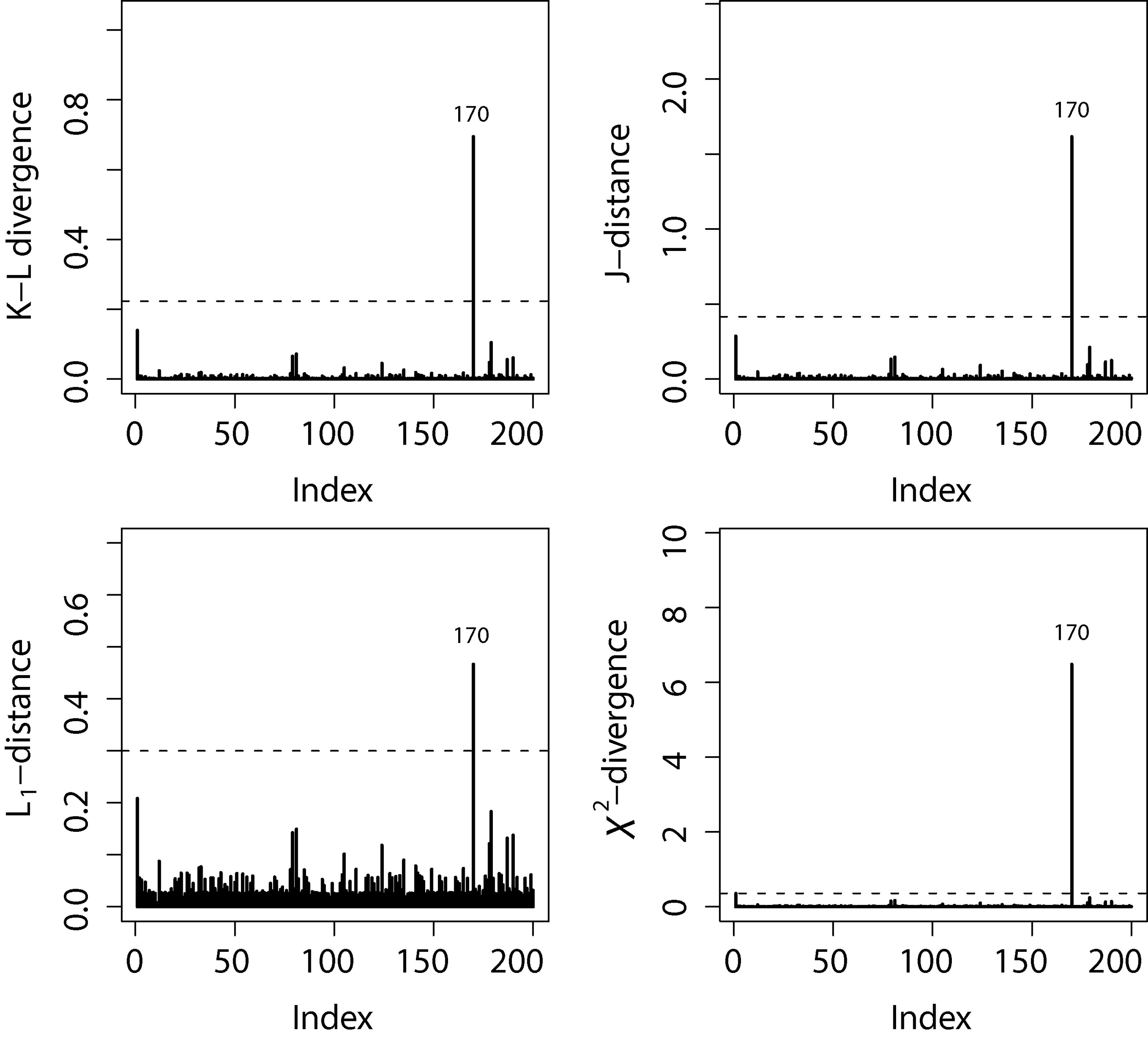
In the Fig. 5, we have depicted the four $\psi$ -divergence measures for the case (d). Clearly we can see that all measures performed well to identifying influential case(s), providing larger $\psi$ -divergence measures when compared to the other cases.

Figure 5.

$\psi$ -divergence measures from dataset (d).

5. Application

In this section we work out an example employing the modeling presented in Section 2. The data set includes 205 patients observed after operation for removal of malignant melanoma in a period of follow up of 15 years. These data are available in the timereg package in R (Scheike, 2009). The observed time $(T)$ ranges from 10 to 5565 days (from 0.0274 to 15.25 years, with mean $=$ 5.9 and standard deviation $=$ 3.1 years) and refers to the time until the patient’s death or the censoring time. Patient dead from other causes, as well as patients still alive at the end of the study are assumed to be censored observations (72%). We take tumor thickness ( $x_{1}$ ) (in mm, mean $=$ 2.92 and standard deviation $=$ 2.96), ulceration status ( $x_{2}$ ) (absent, $n=$ 115; present, $n=$ 90) and sex ( $x_{3}$ ) (female, $n=$ 126; male $n=$ 79) as covariates.

The malignant melanoma is a type of skin cancer which is common worldwide. Even though the exact causes are unknown, as pointed out in Section 2, we may speculate on some possible causes for the malignant melanoma patients data. Although the malignant melanoma seems to be predominantly associated with excessive exposure to sun, it may also arise for individuals who have a history of sunburns and chronic sun exposure. Moreover, various different genes have been identified as risks for developing malignant melanoma (Greene, 1998). In this context, malignant melanoma may also arises in some families with a recognized gene mutation. Besides, multiple genetic events have been related to the disease development (Halachmi & Gilchrest, 2001).

The question here is whether the malignant melanoma occurrence is activated by a first, random or last activation mechanism. That is, a minimum, random or maximum $Z$ is responsible for the production of the event of interest? Moreover here, the cumulative damage in malignant melanoma patients, caused by various unknown causes, may leads to a fatigue process, which may be suitable modeled by a BS distribution (Leiva et al., 2007). In this context, the GBScr models seems to be aligned, offering the possibility of seeking for the more adequate activation mechanism in the light of the data. Furthermore, the Kaplan-Meier estimate of the surviving function is presented in Fig. 7 (upper left panel). The presence of a plateau above 0.6 indicates that models that ignore the possibility of a cure fraction will not be suitable for these data.

Then, we fitted the GBScr models described in Section 2 according to Eqs (4), (7) and (8), crossed with the three simulated mechanisms of activation. For all models the following independent priors were adopted in the Bayesian computations $\beta_{j}\sim N(0,10^{4})$ $j=0,1,2,3$ , $\alpha\sim G(1,0.01)$ and $\lambda\sim G(1,0.01).$ A quantity of 60,000 MCMC posterior samples were used in this analysis after burn-in. We used every twentieth sample from the 60,000 MCMC posterior samples to reduce the autocorrelations and yield better convergence results.

Table 5
Bayesian criteria for the fitted models

	Criterion
Activation	DIC	EAIC	EBIC	LPML
First	423.32	430.90	450.84	$-$ 212.48
Last	434.11	440.31	460.25	$-$ 221.21
Random	428.85	435.28	451.90	$-$ 219.09

To compare the fits of the GBScr model with first, last and random activation mechanisms, we also obtained the values of DIC, EAIC, EBIC and LPML. These criteria of information provide the values presented in Table 5. According to all the criteria, the GBScr model under the first activation mechanism stands out as the best one, which we then select as our working model.

The posterior means, medians, standard deviations and 95% highest posterior density (HPD) intervals for the parameters of the GBScr model under the first activation mechanism are shown in Table 6. The covariates have a significant effect on the reduction of the cured fraction. The maximum likelihood estimates and the corresponding asymptotic 95% intervals in parentheses for the parameters of this models are given by $\hat{\alpha}=$ 1.349 [0.613 , 2.966], $\hat{\lambda}=$ 10.192 [2.066, 50.278] $\hat{\beta}_{\text{intercept}}=$ 1.475 [ 0.312 , 2.637], $\widehat{\beta}_{\text{thickness}}$ $-$ 0.160 [ $-$ 0.263, $-$ 0.057], $\widehat{\beta}_{\text{ulceration}}=$ $-$ 1.395 [ $-$ 2.091, $-$ 0.699] and $\widehat{\beta}_{\text{sex}}=$ $-$ 0.623 [ $-$ 1.272, 0.026]. Comparison between the results shows that the asymptotic 95% confidence intervals turned out to be more conservative than the the Bayesian intervals presented in Table 6. We recall that the Bayesian approach was implemented with minimum prior information.

Table 6

Posterior summaries of the parameters for the Log-1 ${}^{\text{st}}$ model

				HPD Interval (95%)
Parameter	Mean	Median	Standard deviation	LI	LS
$\alpha$	1.339	1.260	0.371	0.845	2.276
$\lambda$	10.758	8.799	6.653	4.355	28.935
$\beta_{\text{intercept}}$	1.597	1.595	0.449	0.714	2.457
$\beta_{\text{thickness}}$	$-$ 0.158	$-$ 0.158	0.053	$-$ 0.264	$-$ 0.054
$\beta_{\text{ulceration}}$	$-$ 1.419	$-$ 1.414	0.367	$-$ 2.111	$-$ 0.711
$\beta_{\text{sex}}$	$-$ 0.626	$-$ 0.627	0.338	$-$ 1.291	0.044

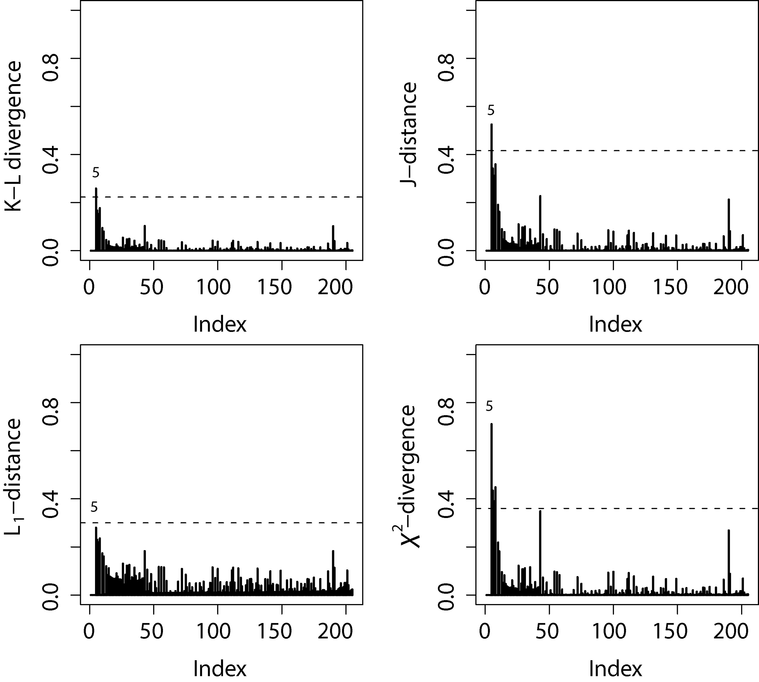
Considering the of the GBScr model under the first activation mechanism the $\psi$ -divergence measures in Eq. (3.3) described in Section 3.3 were computed. The Fig. 6 shows the index plot of the four $\psi$ -divergence measures. For all $\psi$ -divergence measures, the case 5 was identified as the most influential.

Figure 6.

Index plots of $\psi$ -divergence measures for the melanoma data.

The relative changes (in percentage) of each parameter estimate, defined by ${\textit{RC}}_{\vartheta_{j}}=|(\hat{\vartheta}_{j}-\hat{\vartheta}_{j(I)})/% \hat{\vartheta}_{j}|\times 100$ , where $\widehat{\vartheta}_{j(I)}$ denotes the posterior mean of $\vartheta_{j}$ , with $j=1,\ldots,9$ , after the observations $I=\{5\}$ has been removed. The RC in posterior means and the corresponding 95% HPD intervals in parentheses for the parameters of the GBScr model under the first activation mechanism are given by 4.24 [0.815;2.128] for $\alpha$ , 0.170 [4.331;29.362] for $\lambda$ , 4.586 [0.605;2.400] for $\beta_{\text{intercept}}$ , 11.510 [-0.245;-0.0332] for $\beta_{\text{thickness}}$ 1.873 [-2.183;-0.759] for $\beta_{\text{ulceration}}$ and 6.814 [-1.246;0.142] for $\beta_{\text{sex}}$ . We notice that there are little ${RC}$ in posterior mean with exception to $\beta_{\text{thickness}}$ after dropping the observation 5. However, there is no changes in the inferences for the coefficients. Thus, the final selected GBScr model in our analysis has cure rate given by

$p_{0i}=\frac{\exp\left\{\beta_{\text{intercept}}+x_{1i}\beta_{\text{tickness}}% +x_{2i}\beta_{\text{ulceration}}\right\}}{1+\exp\left\{\beta_{\text{intercept}% }+x_{1i}\beta_{\text{tickness}}+x_{2i}\beta_{\text{ulceration}}\right\}},i=1,% \dots,n.$

If follows that the posterior means(standard deviations) and 95% HPD intervals for $\alpha$ , $\beta$ and $\bm{\beta}$ are given by 1.343 (0.361) and [0.857;2.289] for $\alpha$ , 10.384 (6.035) and [4.407;28.081] for $\lambda$ , 1.391 (0.403) and [0.576;2.166] for $\beta_{\text{intercept}}$ , $-$ 0.169 (0.053) and [ $-$ 0.276; $-$ 0.057] for $\beta_{\text{thickness}}$ and $-$ 1.433(0.363) and [ $-$ 2.149; $-$ 0.749] for $\beta_{\text{ulceration}}$ . The values of (DIC, LPML) are (423.85, $-$ 213.09), respectively.

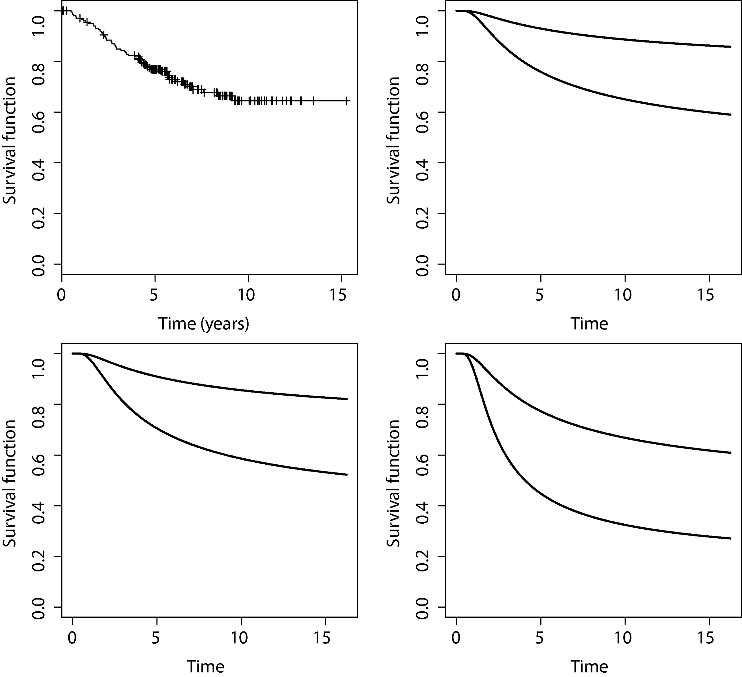
Now we turn our attention to the role of the covariates on the cured fraction $p_{0}$ . Table 7 shows the posterior summaries for the cured fraction stratified by ulceration status with tumor thickness equal to 0.32, 1.94 and 8.32 mm, which correspond to the 5, 50 and 95 percentiles, under the GBScr model under the first activation mechanism. Fig. 7 displays the survival function stratified by ulceration status for patients with tumor thickness equal to 0.32, 1.94 and 8.32 mm. These plots highlight the combined impact of the covariates on the cured fraction. For each selected tumor thickness value the intervals do not overlap.

Figure 7.

Upper left panel: Kaplan-Meier estimate of the surviving function. Surviving function under the GBScr model under the first activation mechanism stratified by ulceration status (upper: absent, lower: present) for patients with tumor thickness equal to 0.64 (upper right panel), 1.94 (lower left panel) and 8.32 mm(lower right panel).

Table 7

Posterior summaries of the cured fraction stratified by ulceration status and selected tumor thickness under GBScr model

Tumor thickness	Ulceration	Mean	Median	Standard deviation	95% HPD interval
0.64	Absent	0.766	0.786	0.067	(0.626, 0.898)
	Present	0.464	0.465	0.094	(0.286, 0.651)
1.94	Absent	0.737	0.748	0.073	(0.577, 0.855)
	Present	0.411	0.412	0.086	(0.251, 0.583)
8.32	Absent	0.564	0.570	0.104	(0.363, 0.752)
	Present	0.245	0.241	0.069	(0.124, 0.391)

We end up our application dealing with the estimation of the proportion of patients non cured who survived beyond a certain fixed time, which is the practical interest to practitioners. For sake of illustration we choose 5 years. This proportion is estimated from ${S}_{\text{GBS}}(5)$ (model under the first activation mechanism) given in Eq. (9). Considering posterior samples of the parameters of the GBScr model, the estimated of Monte Carlo of ${S}_{\text{GBS}}(5)$ stratified by ulceration status (absent, present) for non cured patients with tumor thickness equal to 0.32, 1.94 and 8.32 mm (joint with the posterior standard deviation) are given by (0.600 [0.095], 0.477 [0.085]), (0.585 [0.093], 0.441[0.078]) and (0.484 [0.0.091], 0.273 [0.066]).

6. Concluding remarks

In this paper we proposed the geometric Birnbaum-Saunders cure rate model under different activation mechanisms. Moreover, we propose an influence diagnostic approach from the Bayesian point of view, based on the $\psi$ -divergence (Peng & Dey, 1995; Weiss, 1996) between the posterior distributions of the parameters of the proposed model. Our simulation study indicates that it is possible to discriminate among its particular cases based on the DIC, EAIC, EBIC and LPML criteria. In the application to a melanoma dataset we discovered the GBScr model under the first activation mechanism provides the best fit. Moreover, we observed that the surviving probability decreases more rapidly for patients with thicker tumors, and that the cured fraction is lower for patients with ulceration.

There are some open questions which must be considered further. For instance, we only consider, as usual in the survival literature, that censored observations are subjects who either die of causes other than the disease of interest or are lost during the follow-up. However, as pointed out by a referee, we do not know that deaths from other causes are non informative and can be taken as censored observations. Moreover, the above issue together with the first activation mechanism standing out as an competing risk problem, in which the number of risks as well as the risk responsible for the occurrence of the event of interest are unknown. In this context, which influence could have the other deaths on the results if they were somehow related to T? How would the marginal estimation of $T$ would change and how much the coefficients would be affected? Those questions must be addressed elsewhere.

References

Arellano-Valle

Galea-Rojas

, & Zuazola

P. I.

(2000). Bayesian sensitivity analysis in elliptical linear regression models. Journal of Statistical Planning and Inference, 86(1),175-199.

Balakrishnan

, & Kundu

(2019). Birnbaum-saunders distribution: A review of models, analysis, and applications. Appl Stochastic Models Bus Ind, 35, 4-49.

Berkson

, & Gage

R. P.

(1952). Survival curve for cancer patients following treatment. Journal of the American Statistical Association, 47, 501-515.

Birnbaum

Z. W.

, & Saunders

S. C.

(1969). A new family of life distributions. Journal of Applied Probability, 6(2), 319-327.

Boag

J. W.

(1949). Maximum likelihood estimates of the proportion of patients cured by cancer therapy. Journal of the Royal Statistical Society B, 11, 15-53.

Brooks

S. P.

(2002). Discussion on the paper by Spiegelhalter, Best, Carlin, and van der Linde (2002). Journal of the Royal Statistical Society B, 64, 616-618.

Cancho

Ortega

, & Bolfarine

(2009). The log-exponentiated-weibull regression models with cure rate: Local influence and residual analysis. Journal of Data Science, 7, 433-458.

Cancho

Ortega

, & Paula

(2010). On estimation and influence diagnostics for log-birnbaum-saunders student-t regression models: Full Bayesian analysis. Journal of Statistical Planning and Inference, 140(9), 2486-2496.

Cancho

Dey

Lachos

, & Andrade

(2011). Bayesian nonlinear regression models with scale mixtures of skew-normal distributions: Estimation and case influence diagnostics. Computational Statistics & Data Analysis, 55(1), 588-602.

10.

Cancho

de Castro

, & Rodrigues

(2012a). A bayesian analysis of the conway-maxwell-poisson cure rate model. Statistical Papers, 53, 165-176.

11.

Cancho

Louzada

, & Barriga

(2012b). The geometric Birnbaum-Saunders regression model with cure rate. Journal of Statistical Planning and Inference, pp. 99-1000.

12.

Cancho

Bandyopadhyay

Louzada

, & Yiqi

(2013). The destructive negative binomial cure rate model with a latent activation scheme. Statistical Methodology, 13, 48-68.

13.

Carlin

B. P.

, & Louis

T. A.

(2001). Bayes and Empirical Bayes Methods for Data Analysis. Chapman & Hall/CRC, Boca Raton, second edition.

14.

Carlin

B. P.

, & Polson

N. G.

(1991). An expected utility approach to influence diagnostics. Journal of the American Statistical Association, 86(416), 1013-1021.

15.

Cho

Ibrahim

J. G.

Sinha

, & Zhu

(2009). Bayesian case influence diagnostics for survival models. Biometrics, 65(1), 116-124.

16.

Cook

R. D.

(1986). Assessment of local influence. Journal of the Royal Statistical Society, Series B, 48, 133-169.

17.

Cook

R. D.

, & Weisberg

(1982). Residuals and Influence in Regression. Chapman & Hall/CRC, Boca Raton, FL.

18.

Cooner

Banerjee

, & McBean

A. M.

(2006). Modelling geographically referenced survival data with a cure fraction. Statistical Methods in Medical Research, 15, 307-324.

19.

Cooner

Banerjee

Carlin

B. P.

, & Sinha

(2007). Flexible cure rate modeling under latent activation schemes. Journal of the American Statistical Association, 102, 560-572.

20.

Cowles

M. K.

, & Carlin

B. P.

(1996). Markov chain Monte Carlo convergence diagnostics: A comparative review. Journal of the American Statistical Association, 91, 883-904.

21.

Cox

D. R.

, & Hinkley

D. V.

(1979). Theoretical statistics. Chapman & Hall/CRC.

22.

Dey

, & Birmiwal

(1994). Robust bayesian analysis using divergence measures. Statistics & Probability Letters, 20(4), 287-294.

23.

Dey

Chen

, & Chang

(1997). Bayesian approach for nonlinear random effects models. Biometrics, pp. 1239-1252.

24.

Díaz-García

J. A.

, & Leiva-Sánchez

(2005). A new family of life distributions based on the elliptically contoured distributions. Journal of Statistical Planning and Inference, 128(2), 445-457.

25.

Geisser

, & Eddy

(1979). A predictive approach to model selection. Journal of the American Statistical Association, pp. 153-160.

26.

Gelfand

Dey

, & Chang

(1992). Model determination using predictive distributions with implementation via sampling based methods (with discussion). bayesian statistics 4. eds: Bernardo

et al. JM

Bernardo

Berger

Dawid

AFM

Smith

(editors). Oxford University Press, 1(4), 7-167.

27.

Gelfand

A. E.

, & Smith

A. F.

(1990). Sampling-based approaches to calculating marginal densities. Journal of the American Statistical Association, 85(410), 398-409.

28.

Geweke

(1992). Evaluating the accuracy of sampling-based approaches to the calculation of posterior moments. bayesian statistics 4. eds: J. bernardo et al. Bernardo

J M

Berger

J O

Dawid

A P

Smith

AFM

(editors). Oxford University Press, 1(4), 169-188.

29.

Gómez

H. W.

Olivares-Pacheco

J. F.

, & Bolfarine

(2009). An extension of the generalized Birnbaum-Saunders distribution. Statistics and Probability Letters, 79(3), 331-338.

30.

Greene

M. H.

(1998). The genetics of hereditary melanoma and nevi. Cancer, 86(11), 2464-2477.

31.

Halachmi

, & Gilchrest

B. A.

(2001). Update on genetic events in the pathogenesis of melanoma. Current Opinion in Oncology, 13(2), 129-136.

32.

Ibrahim

J. G.

Chen

M.-H.

, & Sinha

(2001). Bayesian Survival Analysis. Springer, New York.

33.

Kim

Chen

, & Dey

(2011). A new threshold regression model for survival data with a cure fraction. Lifetime data analysis, 17(1), 101-122.

34.

Leiva

Barros

Paula

, & Galea

(2007). Influence diagnostics in log-birnbaum-saunders regression models with censored data. Computational Statistics & Data Analysis, 51(12), 5694-5707.

35.

C. S.

Taylor

J. M.

, & Sy

J. P.

(2001). Identifiability of cure models. Statistics and Probability Letters, 54, 389-395.

36.

Maller

R. A.

, & Zhou

(1996). Survival Analysis with Long-Term Survivors. Wiley, New York.

37.

Peng

, & Dey

(1995). Bayesian analysis of outlier problems using divergence measures. Canadian Journal of Statistics, 23(2), 199-213.

38.

Pettit

(1986). Diagnostics in bayesian model choice. The Statistician, pages 183-190.

39.

R Development Core Team (2010). R: A Language and Environment for Statistical Computing. R Foundation for Statistical Computing, Vienna, Austria.

40.

Rodrigues

Cancho

V. G.

de Castro

, & Louzada-Neto

(2009). On the unification of the long-term survival models. Statistics & Probability Letters, 79, 753-759.

41.

Sanhueza

Leiva

, & Balakrishnan

(2008). The Generalized Birnbaum-Saunders Distribution and Its Theory, Methodology, and Application. Communications in Statistics-Theory and Methods, 37(5), 645-670.

42.

Scheike

(2009). timereg package. R package version 1.1-0. With contributions from T. Martinussen and J. Silver. R package version 1.1-6.

43.

Spiegelhalter

D. J.

Best

N. G.

Carlin

B. P.

, & van der Linde

. (2002). Bayesian measures of model complexity and fit. Journal of the Royal Statistical Society B, 64, 583-639.

44.

Suzuki

Cancho

, & Louzada

(2016). The poisson-inverse-gaussian regression model with cure rate: a bayesian approach and its case influence diagnostics. Statistical Papers, 57, 133-159.

45.

Suzuki

Barriga

Louzada

, & Cancho

(2017). A general long-term aging model with different underlying activation mechanisms: Modeling, bayesian estimation and case influence diagnostics. Communications in Statistics – Theory and Methods, 46, 3080-3098.

46.

Tsionas

E. G.

(2001). Bayesian inference in Birnbaum-Saunders regression. Communications in Statistics-Theory and Methods, 30(1), 179-193.

47.

Tsodikov

A. D.

Ibrahim

J. G.

, & Yakovlev

A. Y.

(2003). Estimating cure rates from survival data: An alternative to two-component mixture models. Journal of the American Statistical Association, 98, 1063-1078.

48.

Weiss

(1996). An approach to bayesian sensitivity analysis. Journal of the Royal Statistical Society. Series B (Methodological), pages 739-750.

49.

Weiss

R. E.

, & Cook

R. D.

(1992). A graphical case statistic for assessing posterior influenceo. Biometrika, 79(1), 51-55.

50.

, & Tang

(2011). Bayesian analysis of Birnbaum-Saunders distribution with partial information. Computational Statistics & Data Analysis, 55(7), 2324-2333.

51.

Yakovlev

A. Y.

, & Tsodikov

A. D.

(1996). Stochastic Models of Tumor Latency and Their Biostatistical Applications. World Scientific, Singapore.

Bayesian analysis of Birnbaum-Saunders survival model with cure fraction under a variety of activation mechanism

Abstract

Keywords

1. Introduction

.

4.1 Frequentist properties

Table 1 Simulation summary statistics for the cured fraction parameters assuming the models described in in Eqs (4), (7) and (8), crossed with the three mechanisms of activation simulated based on 500 Monte Carlos datasets

Table 3 Mean, Standard Deviation(SD) and Bayesian criteria of the GBScr model parameters under a first activation mechanism for each datasets

Table 5 Bayesian criteria for the fitted models

References

Table 1
Simulation summary statistics for the cured fraction parameters assuming the models described in in Eqs (4), (7) and (8), crossed with the three mechanisms of activation simulated based on $500$ Monte Carlos datasets

Table 3
Mean, Standard Deviation(SD) and Bayesian criteria of the GBScr model parameters under a first activation mechanism for each datasets

Table 5
Bayesian criteria for the fitted models