The application of predictive distribution estimation in multiple-inflated poisson models to ice hockey data

Abstract

In this paper, we introduce a multiple-inflated Poisson distribution that can handle count data with multiple inflated values. We explore a Bayes predictive distribution for future observation under Kullback Leibler loss function and a class of shrinkage priors, along with plug-in type pmf estimators. To illustrate how well the proposed pmf estimators perform, we provide both a simulated study and a real example analyzing a dataset of National Hockey League (NHL) shootout losses in 2017/18.

Keywords

Bayes predictive distribution estimation count data Kullback Leibler loss function multiple-inflated poisson distribution plug-in pmf estimator shrinkage prior

1. Introduction

Often the times discrete frequency distributions involve counts of occurrences of events, such as the number of goals in a match, accident fatalities, suicides or insurance claims. The most commonly used model to analyze this kind of data is a Poisson distribution. However, in many practical situations, the Poisson distribution fails to model count data which exhibits over-dispersion (i.e., the variance exceeds the mean). Furthermore, another situation that makes the Poisson distribution less applicable is the excess number of zeros in a dataset (zero-inflation).

The zero-inflated model ( $\operatorname{ZIP}$ ) is used where the observed number of zeros exceeds that which is expected by a Poisson distribution (see Mullahy, 1986; Lambert, 1992). There are many situations that the $\operatorname{ZIP}$ model is used; for example, in insurance (Yip & Yau, 2005), industry and manufacturing processes (Ghosh et al., 2006), health insurance (Mouatassim & Ezzahid, 2012) and public health data (Unhapipat, 2018).

In addition, some data sets may have multiple inflated counts of additional value rather than zero (multiple-inflation) and bulking of certain values can happen. For example, in datasets such as the number of red (or yellow) cards in the Premier League, penalties taken in certain season national hockey league (NHL), times a woman received a mammogram in the past two years, or days in week someone drinks alcohol, we would expect to see excess zeros and/or ones that we do not expect to see in the Poisson model. Lin and Tsai (2016) have discussed a model that can be applied to both excessive zeros and ones known as the zero-and-one-inflated Poisson, or ( $\operatorname{ZOIP}$ ), model.

This paper considers predictive estimation of future probability mass function (pmf) in a multiple-inflated Poisson model, and, more specifically, a model that can be applied to a dataset with two inflated values, namely $k_{1}$ and $k_{2}$ . This model embraces all the inflated Poisson models and can be extended to $k_{i}$ inflated values, for $i\geqslant 2$ .

The remainder of the article is organized as follows. In Section 2, we introduce the multiple-inflated Poisson models along with the corresponding likelihood function. Section 3 addresses the Bayesian setup and we discuss how to find the Bayesian predictive distribution under the Kullback Leibler loss function and the improper shrinkage prior. In Section 4, by simulating the inflated data, we compare the proposed Bayes predictive distribution with other kinds of pmf estimators called plug-in pmf estimators. In Section 5, we apply our obtained pmf estimators to real data from a hockey game. Finally, we make some concluding remarks in Section 6.

2. Problem set-up

One of the simplest methods for modeling count data is the Poisson distribution, denoted by $\operatorname{Po}(\lambda)$ , with the pmf

$\displaystyle P(X=x\mid\lambda)=\frac{e^{-\lambda}\lambda^{x}}{x!},x=0,1,% \ldots,\lambda>0.$ (1)

The pmf in Eq. (1) gives the probability of the event occurring over a large number of independent trials (in time or space), when the probability of that the event occurs on any one trial is small and constant. Therefore, the Poisson distribution is often used to model rare events such as highway accidents, earthquakes, incidents of terrorism, or the number of particles emitted from a small radioactive sample. The variance in the Poisson model Eq. (1) is identical to the mean ( $=\lambda$ ), thus making the variance equal one.

Another distribution that might be used in modelling of count data which permits the over-dispersion is a negative binomial distribution. A random variable $X\sim\operatorname{NB}(r,p)$ has the pmf

$\displaystyle P(X=k)=\binom{k+r-1}{k}(1-p)^{r}p^{k},x=0,1,\ldots,$ (2)

The pmf in Eq. (2) shows the probability of a certain number of independent events occurring prior to a specific amount of failures. The mean and variance of the negative binomial distribution in Eq. (2) are $r(1-p)/p$ and $r(1-p)/p^{2}$ respectively, and the variance is greater than the mean.

The distribution in Eq. (2) can be considered a gamma mixture of Poisson distributions. If we let $\lambda$ in Eq. (1) follows the gamma distribution $\operatorname{Gam}(r,\beta=\frac{1-p}{p})$ , with the probability density function (pdf) $\frac{\beta^{r}}{\Gamma(r)}\lambda^{r-1}e^{-\beta\lambda}$ , for $r>0,\lambda>0$ and $\beta>0$ , then the resulting distribution is the negative binomial as in Eq. (2). Note that as $r\to\infty$ , the pmf in Eq. (2) tends to Eq. (1).

In addition to over-dispersion, often datasets exhibit more zero or other observations than would be allowed for by the Poisson model or even the negative binomial.

A $\operatorname{ZIP}(p,\lambda)$ distribution is a two-component mixture model combining a point mass at zero with a Poisson distribution and it has the pmf

$\displaystyle P(X=x\mid p,\lambda)=\begin{cases}p+(1-p)e^{-\lambda}&\text{if }% x=0\\ (1-p){\displaystyle\frac{e^{-\lambda}\lambda^{x}}{x!}}&\text{if }x\in\mathbb{N% }.\end{cases}$ (3)

The extra parameter $0<p<1$ in Eq. (3) is called the inflation parameter (at 0) which, along with parameter $\lambda$ , is unknown. The idea of the inflated probability at zero can be extended to another count value, such as $k$ . The $k$ –inflated Poisson, $\operatorname{KIP}$ , arises when the probability is inflated at value $k$ . The pmf of $\operatorname{KIP}(p,\lambda)$ is

$\displaystyle P(X=x\mid p,\lambda)=\begin{cases}p+(1-p){\displaystyle\frac{e^{% -\lambda}\lambda^{k}}{k!}}&\text{if }x=k\\ (1-p){\displaystyle\frac{e^{-\lambda}\lambda^{x}}{x!}}&\text{if }x\in\mathbb{N% }\setminus\{k\}.\end{cases}$ (4)

The $\operatorname{KIP}$ model in Eq. (4) reduces to the $\operatorname{ZIP}$ model in Eq. (3) whenever $k=0$ and the Poisson distribution corresponds to $p=0$ . The multiple-inflate $\operatorname{K_{1}K_{2}IP}$ model, is a generalization of the $\operatorname{KIP}$ model, including two inflations, $x=k_{1}$ and $x=k_{2}$ , comparing to the Poisson distribution. The pmf of ${K_{1}K_{2}IP}(p_{1},p_{2},\lambda)$ is given as follows:

$\displaystyle P(X=x\mid p_{1},p_{2},\lambda)=\begin{cases}p_{1}+p_{3}{% \displaystyle\frac{e^{-\lambda}\lambda^{k_{1}}}{k_{1}!}}&\text{if }x=k_{1}\\ p_{2}+p_{3}{\displaystyle\frac{e^{-\lambda}\lambda^{k_{2}}}{k_{2}!}}&\text{if % }x=k_{2}\\ p_{3}{\displaystyle\frac{e^{-\lambda}\lambda^{x}}{x!}}&\text{if }x\in\mathbb{N% }\setminus\{k_{1},k_{2}\},\end{cases}$ (5)

where $p_{3}=1-p_{1}-p_{2}$ . An intuitive approach to obtain the pmf in Eq. (5) is to define a latent variable $Z$ which is distributed as a multinomial with $P(Z=z_{i})=p_{i}$ , for $i=1,2,3$ , where $0<p_{i}<1$ , and $p_{3}=1-p_{1}-p_{2}$ . This implies

$\displaystyle P(X=x\mid p_{1},p_{2},\lambda,z_{1},z_{2},z_{3})=\begin{cases}1&% \text{if }x=k_{1},z=z_{1}\\ 1&\text{if }x=k_{2},z=z_{2}\\ {\displaystyle\frac{e^{-\lambda}\lambda^{x}}{x!}}&\text{if }x\in\mathbb{N}% \setminus\{k_{1},k_{2}\},z=z_{3}.\end{cases}$ (6)

Therefore, the joint pmf of $X$ and $Z_{1},Z_{2},Z_{3}$ is given by

$\displaystyle P(X=x,Z_{1}=z_{1},Z_{2}=z_{2},Z_{3}=z_{3}\mid p_{1},p_{2},% \lambda)=\begin{cases}p_{1}&\text{if }x=k_{1},z=z_{1}\\ p_{2}&\text{if }x=k_{2},z=z_{2}\\ p_{3}{\displaystyle\frac{e^{-\lambda}\lambda^{x}}{x!}}&\text{if }x\in\mathbb{N% }\setminus\{k_{1},k_{2}\},z=z_{3},\end{cases}$ (7)

and the marginal pmf of $X$ is therefore modeled in Eq. (5).

2.1 Likelihood functions

Let us suppose that data points from the $K_{1}K_{2}IP$ model, i.e., $n_{k_{1}}$ and $n_{k_{2}}$ , the number of $x_{i}=k_{1}$ and $x_{i}=k_{2}$ for $i=1,\ldots,n$ , are quite large. If $x=(x_{1},\ldots,x_{n})$ and $n_{3}=n-n_{k_{1}}-n_{k_{2}}$ , then the likelihood function is given by

$\displaystyle L(p_{1},p_{2},\lambda\mid x)\propto\left(p_{1}+p_{3}e^{-\lambda}% \frac{\lambda^{k_{1}}}{k_{1}!}\right)^{n_{k_{1}}}\left(p_{2}+p_{3}e^{-\lambda}% \frac{\lambda^{k_{2}}}{k_{2}!}\right)^{n_{k_{2}}}p_{3}^{n_{3}}e^{-n_{3}\lambda% }\lambda^{\sum\limits_{\{i:x_{i}\neq k_{1},k_{2}\}}\!\!\!\!x_{i}}\propto\sum_{% j=0}^{n_{k_{1}}}\binom{n_{k_{1}}}{j}p_{1}^{j}p_{3}^{n_{k_{1}}-j}e^{-k_{1}(n_{k% _{1}}-j)}\sum_{l=0}^{n_{k_{2}}}\binom{n_{k_{2}}}{l}p_{2}^{l}p_{3}^{n_{k_{2}}-l% }e^{-k_{2}(n_{k_{2}}-l)}p_{3}^{n_{3}}e^{\lambda n_{3}}\lambda^{\sum\limits_{\{% i:x_{i}\neq k_{1},k_{2}\}}\!\!\!\!x_{i}}\propto\sum_{j=0}^{n_{k_{1}}}\binom{n_% {k_{1}}}{j}\sum_{l=0}^{n_{k_{2}}}\binom{n_{k_{2}}}{2}p_{1}^{j}p_{1}^{l}p_{3}^{% n-j-l}e^{-\lambda(n-j-l)}\lambda^{\sum\limits_{\{i:x_{i}\neq k_{1},k_{2}\}}\!% \!\!\!x_{i}+k_{1}(n_{k_{1}}-j)+k_{2}(n_{k_{2}}-l)}.$ (8)

For the KIP $(p,\lambda)$ model in Eq. (4), we have

$\displaystyle L(p,\lambda\mid x)\propto\left(p+(1-p)e^{-\lambda}\frac{\lambda^% {k}}{k!}\right)^{n_{k}}(1-p)^{n-n_{k}}e^{-(n-n_{k})\lambda}\lambda^{\sum_{\{i:% x_{i}\neq k\}}x_{i}}\propto\sum_{j=0}^{n_{k}}\binom{n_{k}}{j}p^{j}(1-p)^{n-j}e% ^{-\lambda(n-j)}\lambda^{\sum\limits_{\{i:x_{i}\neq k\}}x_{i}+k(n_{k}-j)}.$ (9)

Remark 1. The maximum likelihood estimator (mle) of unknown parameters $p_{1}$ , $p_{2}$ and $\lambda>0$ in the $\operatorname{K_{1}K_{2}IP}(p_{1},p_{2},\lambda)$ model can be obtained numerically by considering the constraints $0<p_{1}<0$ , $0<p_{2}<1$ , $p_{1}+p_{2}<1$ and $\lambda>0$ from Eq. (8). Similarly, one can use Eq. (9) to find the mle of parameter $p$ and $\lambda$ in the $\operatorname{KIP}(p_{1},p_{2},\lambda)$ model.

We need the following definition to set up a Bayesian framework.

Definition 1. Consider the bounded continuous variate $\mathbf{t}=(t_{1},\ldots,t_{m})$ , such that $0<t_{i}<m-1$ and $t_{m}=1-\sum_{i=0}^{m-1}t_{i}<1$ . The Dirichlet distribution is given as

$\displaystyle P(\mathbf{T}=\mathbf{t}\mid\bm{\gamma})=D(\bm{\gamma})\prod_{i=1% }^{m}t_{i}^{\gamma_{i}-1},$ (10)

where $D(\bm{\gamma})=\frac{\prod_{i=1}^{m}\Gamma(\gamma_{i})}{\Gamma(\sum_{i=1}^{m}% \gamma_{i})}$ and $\bm{\gamma}=(\gamma_{1},\ldots,\gamma_{m})$ . Note that the beta distribution is equivalent to a bivariate Dirichlet distribution with $t_{1}=t$ and $t_{2}=1-t$ , and thus, $D(\alpha_{1},\alpha_{2})=\operatorname{Bet}(\alpha_{1},\alpha_{2})$ .

3. Bayesian set-up

3.1 Prior and posterior densities

Komaki (2004) introduced a class of improper shrinkage prior for the mean of Poisson distributions as

$\displaystyle\pi(\lambda)\propto\lambda^{\beta-\alpha-1},\lambda>0,\beta>0,0<% \alpha<\beta.$ (11)

Jeffreys prior corresponds to $\alpha=0$ and $\beta=\frac{1}{2}$ . Let us assume that $\mathbf{p}=(p_{1},p_{2},p_{3})$ and $p_{i}\sim U(0,1)$ ; $i=1,2$ , $\lambda\sim\pi(\lambda)$ , with the pdf as in Eq. (11), be independent, respectively. The following Lemma provides the posterior density $\mathbf{p},\lambda$ given $x$ .

Lemma 1. (i) Suppose that $X\sim\operatorname{K_{1}K_{2}IP}(p_{1},p_{2},\lambda)$ , and that prior densities $p_{i}\sim U(0,1)$ and $\lambda\sim\pi(\lambda)$ as in Eq. (11) are independent respectively. Then the posterior density, by assuming

$\displaystyle w_{j,l}(x)=\sum\limits_{\{i:x_{i}\neq k_{1},k_{2}\}}\!\!\!\!x_{i% }+k_{1}(n_{k_{1}}-j)+k_{2}(n_{k_{2}}-l)+\beta-\alpha-1,$ (12)

is given by

$\displaystyle\pi(\mathbf{p},\lambda\mid x)=\frac{\sum\limits_{j=0}^{n_{k_{1}}}% \sum\limits_{l=0}^{n_{k_{2}}}\binom{n_{k_{1}}}{j}\binom{n_{k_{2}}}{l}p_{1}^{j}% p_{2}^{l}p_{3}^{n-j-l}e^{-\lambda(n-j-l)}\lambda^{w_{j,l}(x)}}{\sum\limits_{j=% 0}^{n_{k_{1}}}\sum\limits_{l=0}^{n_{k_{2}}}\binom{n_{k_{1}}}{j}\binom{n_{k_{2}% }}{l}D(l+1,j+1,n-j-l+1)\Gamma(w_{j,l}(x)+1)(n-j-l)^{-w_{j,l}(x)-1}},$ (13)

for $0<p_{1}<1$ , $0<p_{2}<1$ , $0<1-p_{1}-p_{2}<1$ and $\lambda>0$ .

(ii) Suppose that $x\sim\operatorname{KIP}(p,\lambda)$ , and prior densities are $p\sim U(0,1)$ and $\lambda\sim\pi(\lambda)$ as in Eq. (11) are independent respectively. Then the posterior density by assuming

$\displaystyle w_{j}(x)=\sum\limits_{\{i:x_{i}\neq k\}}x_{i}+\beta-\alpha+k(n_{% k}-j)-1,$ (14)

is given by

$\displaystyle\pi(p,\lambda\mid x)=\frac{\sum\limits_{j=0}^{n_{k}}\binom{n_{k}}% {j}p^{j}(1-p)^{n-j}e^{-(n-j)\lambda}\lambda^{w_{j}(x)}}{\sum\limits_{j=0}^{n_{% k}}\binom{n_{k}}{j}\operatorname{Bet}(j+1,n-j+1)\Gamma(w_{j}(x)+1)(n-j)^{-w_{j% }(x)-1}}.$ (15)

Proof Part (i). By replacing likelihood function Eq. (8) and priors in the posterior density formula, we can write

$\displaystyle\pi(\mathbf{p},\lambda\mid x)=\frac{L(\mathbf{p},\lambda\mid x)% \pi(\lambda)}{\int_{0}^{1}\int_{0}^{1}\int_{0}^{\infty}L(\mathbf{p},\lambda% \mid x)\pi(\lambda)d\lambda d\mathbf{p}}.$ (16)

The denominator in Eq. (16) can be written as

$\displaystyle\int_{0}^{1}\int_{0}^{1}\int_{0}^{\infty}\sum\limits_{j=0}^{n_{k_% {1}}}\binom{n_{k_{1}}}{j}\sum\limits_{l=0}^{n_{k_{2}}}\binom{n_{k_{2}}}{2}p_{1% }^{j}p_{1}^{l}p_{3}^{n-j-l}e^{-\lambda(n-j-l)}\lambda^{\sum\limits_{\{i:x_{i}% \neq k_{1},k_{2}\}}\!\!\!\!x_{i}+k_{1}(n_{k_{1}}-j)+k_{2}(n_{k_{2}}-l)}d% \lambda d\mathbf{p}$ (17)

Applying Definition 1 to Eq. (17), yields

$\displaystyle\sum\limits_{j=0}^{n_{k_{1}}}\sum\limits_{l=0}^{n_{k_{2}}}\binom{% n_{k_{1}}}{j}\binom{n_{k_{2}}}{l}D(l+1,j+1,n-j-l+1)\Gamma(w_{j,l}(x)+1)(n-j-l)% ^{-w_{j,l}(x)-1},$

and this completes the proof.

Part (ii). Substituting likelihood function Eq. (9) and priors in the posterior density formula, we have

$\displaystyle\pi(p,\lambda\mid x)=\frac{L(p,\lambda\mid x)\pi(\lambda)}{\int_{% 0}^{1}\int_{0}^{\infty}L(p,\lambda\mid x)\pi(\lambda)d\lambda dp}.$ (18)

The denominator in Eq. (18) can be written as

$\displaystyle\int_{0}^{1}\int_{0}^{\infty}\sum\limits_{j=0}^{n_{k}}\binom{n_{k% }}{j}p^{j}(1-p)^{n-j}e^{-\lambda(n-j)}\lambda^{w_{j}(x)}d\lambda dp$ $\displaystyle=\sum_{j=0}^{n_{k}}\binom{n_{k}}{j}\operatorname{Bet}(j+1,n-j+1)% \int_{0}^{\infty}\lambda^{w_{j}(x)}e^{-\lambda(n-j)}d\lambda$ $\displaystyle=\sum\limits_{j=0}^{n_{k}}\binom{n_{k}}{j}\operatorname{Bet}(j+1,% n-j+1){\displaystyle\frac{\Gamma(w_{j}(x)+1)}{(n-j)^{w_{j}(x)+1}}}.$

Remark 2. The Bayes estimator of $\theta$ , under the squared error loss function $(\hat{\theta}-\theta)^{2}$ , where $\theta$ can be chosen as any of parameters $p_{1}$ , $p_{2}$ and $\lambda>0$ is known to be $\mathbb{E}(\theta\mid X=x)$ . According to the posterior distribution Eq. (15), the corresponding estimators for the $\operatorname{K_{1}K_{2}IP}(p_{1},p_{2},\lambda)$ model are given as follows:

$\displaystyle\hat{p}_{1\pi}=\frac{\sum\limits_{j=0}^{n_{k_{1}}}\sum\limits_{l=% 0}^{n_{k_{2}}}\binom{n_{k_{1}}}{j}\binom{n_{k_{2}}}{l}D(l+1,j+2,n-j-l+1)\Gamma% (w_{j,l}(x)+1)(n-j-l)^{-w_{j,l}(x)-1}}{\sum\limits_{j=0}^{n_{k_{1}}}\sum% \limits_{l=0}^{n_{k_{2}}}\binom{n_{k_{1}}}{j}\binom{n_{k_{2}}}{l}D(l+1,j+1,n-j% -l+1)\Gamma(w_{j,l}(x)+1)(n-j-l)^{-w_{j,l}(x)-1}},$ $\displaystyle\hat{p}_{2\pi}=\frac{\sum\limits_{j=0}^{n_{k_{1}}}\sum\limits_{l=% 0}^{n_{k_{2}}}\binom{n_{k_{1}}}{j}\binom{n_{k_{2}}}{l}D(l+2,j+1,n-j-l+1)\Gamma% (w_{j,l}(x)+1)(n-j-l)^{-w_{j,l}(x)-1}}{\sum\limits_{j=0}^{n_{k_{1}}}\sum% \limits_{l=0}^{n_{k_{2}}}\binom{n_{k_{1}}}{j}\binom{n_{k_{2}}}{l}D(l+1,j+1,n-j% -l+1)\Gamma(w_{j,l}(x)+1)(n-j-l)^{-w_{j,l}(x)-1}},$ $\displaystyle\hat{\lambda}_{\pi}=\frac{\sum\limits_{j=0}^{n_{k_{1}}}\sum% \limits_{l=0}^{n_{k_{2}}}\binom{n_{k_{1}}}{j}\binom{n_{k_{2}}}{l}D(l+1,j+1,n-j% -l+1)\Gamma(w_{j,l}(x)+2)(n-j-l)^{-w_{j,l}(x)-2}}{\sum\limits_{j=0}^{n_{k_{1}}% }\sum\limits_{l=0}^{n_{k_{2}}}\binom{n_{k_{1}}}{j}\binom{n_{k_{2}}}{l}D(l+1,j+% 1,n-j-l+1)\Gamma(w_{j,l}(x)+1)(n-j-l)^{-w_{j,l}(x)-1}}.$

Also, for the model $\operatorname{KIP}(p,\lambda)$ , we have

$\displaystyle\hat{p}_{\pi}=\frac{\sum\limits_{j=0}^{n_{k}}\binom{n_{k}}{j}% \operatorname{Bet}(j+2,n-j+1)\Gamma(w_{j}(x)+1)(n-j)^{-w_{j}(x)-1}}{\sum% \limits_{j=0}^{n_{k}}\binom{n_{k}}{j}\operatorname{Bet}(j+1,n-j+1)\Gamma(w_{j}% (x)+1)(n-j)^{-w_{j}(x)-1}},$ $\displaystyle\hat{\lambda}_{\pi}=\frac{\sum\limits_{j=0}^{n_{k}}\binom{n_{k}}{% j}\operatorname{Bet}(j+1,n-j+1)\Gamma(w_{j}(x)+2)(n-j)^{-w_{j}(x)-2}}{\sum% \limits_{j=0}^{n_{k}}\binom{n_{k}}{j}\operatorname{Bet}(j+1,n-j+1)\Gamma(w_{j}% (x)+1)(n-j)^{-w_{j}(x)-1}}.$

3.2 Bayes predictive distributions

We consider the problem of constructing the Bayes predictive distribution for the future observation $y$ , based on observable $x$ . We use the Kullback Leibler (KL) loss function (divergence)

$\displaystyle\operatorname{KL}(q(y\mid\theta)),\hat{q}_{\pi}(y;x))=\sum_{y}q(y% \mid\theta)\log\frac{q(y\mid\theta)}{\hat{q}_{\pi}(y;x)},$ (19)

where $\hat{q}_{\pi}(y;x)$ is the Bayes predictive distribution for estimating the pmf $Y\sim q(\cdot\mid\theta)$ , and $\theta$ is a (n) (vector of) unknown parameter (s). The corresponding risk function given as follows

$\displaystyle r_{\hat{q}}(\theta)=\mathbb{E}^{x\mid\theta}\operatorname{KL}(q,% \hat{q})=\sum_{x}q(x\mid\theta)\sum_{y}q_{\theta}(y)\log\frac{q(y\mid\theta)}{% \hat{q}_{\pi}(y;x)}.$ (20)

Previous studies (see Corcuera & Giummolè, 1999) indicate that under KL, the Bayes predictive distribution for $Y$ , based on observed value $x$ , and posterior density $\pi(\cdot\mid x)$ , is given as

$\displaystyle\hat{q}_{\pi}(y;x)=\int_{\Theta}q(y\mid\theta)\pi(\theta\mid x)d\theta.$ (21)

The following theorem provides the Bayes predictive distribution under KL loss function.

Theorem 1. The Bayes predictive distribution of future observation $y$ based on observable $x=(x_{1},\ldots,x_{n})$ from

(i) the $\operatorname{K_{1}K_{2}IP}(\mathbf{p,\lambda})$ model, in Eq. (5), with priors defined in Lemma 1 (i), is given by

$\displaystyle\hat{q}(Y=k_{1};x)=\frac{\sum\limits_{j=0}^{n_{k_{1}}}\sum\limits% _{l=0}^{n_{k_{2}}}\binom{n_{k_{1}}}{j}\binom{n_{k_{2}}}{l}(n-j-l+1)^{-w_{j,l}(% x)-k_{1}-1}D(l+1,j+1,n-j-l+2)\Gamma(w_{j,l}(x)+k_{1}+1)}{k_{1}!\sum\limits_{j=% 0}^{n_{k_{1}}}\sum\limits_{l=0}^{n_{k_{2}}}\binom{n_{k_{1}}}{j}\binom{n_{k_{2}% }}{l}(n-j-l)^{-w_{j,l}(x)-1}D(l+1,j+1,n-j-l+1)\Gamma(w_{j,l}(x)+1)}+\frac{\sum% \limits_{j=0}^{n_{k_{1}}}\sum\limits_{l=0}^{n_{k_{2}}}\binom{n_{k_{1}}}{j}% \binom{n_{k_{2}}}{l}(n-j-l)^{-w_{j,l}(x)-1}D(l+1,j+2,n-j-l+1)\Gamma(w_{j,l}(x)% +1)}{\sum\limits_{j=0}^{n_{k_{1}}}\sum\limits_{l=0}^{n_{k_{2}}}\binom{n_{k_{1}% }}{j}\binom{n_{k_{2}}}{l}(n-j-l)^{-w_{j,l}(x)-1}D(l+1,j+1,n-j-l+1)\Gamma(w_{j,% l}(x)+1)},\hat{q}(Y=k_{2};x)=\frac{\sum\limits_{j=0}^{n_{k_{1}}}\sum\limits_{l% =0}^{n_{k_{2}}}\binom{n_{k_{1}}}{j}\binom{n_{k_{2}}}{l}(n-j-l+1)^{-w_{j,l}(x)-% k_{2}--1}D(l+1,j+1,n-j-l+2)\Gamma(w_{j,l}(x)+k_{2}+1)}{k_{2}!\sum\limits_{j=0}% ^{n_{k_{1}}}\sum\limits_{l=0}^{n_{k_{2}}}\binom{n_{k_{1}}}{j}\binom{n_{k_{2}}}% {l}(n-j-l)^{-w_{j,l}(x)-1}D(l+1,j+1,n-j-l+1)\Gamma(w_{j,l}(x)+1)}+\frac{\sum% \limits_{j=0}^{n_{k_{1}}}\sum\limits_{l=0}^{n_{k_{2}}}\binom{n_{k_{1}}}{j}% \binom{n_{k_{2}}}{l}(n-j-l)^{-w_{j,l}(x)-1}D(l+2,j+1,n-j-l+1)\Gamma(w_{j,l}(x)% +1)}{\sum\limits_{j=0}^{n_{k_{1}}}\sum\limits_{l=0}^{n_{k_{2}}}\binom{n_{k_{1}% }}{j}\binom{n_{k_{2}}}{l}(n-j-l)^{-w_{j,l}(x)-1}D(l+1,j+1,n-j-l+1)\Gamma(w_{j,% l}(x)+1)},$ (23)

and for $y\in\mathbb{N}\setminus\{k_{1},k_{2}\}$ , we have

$\displaystyle\hat{q}(Y=y;x)={\displaystyle\frac{\sum\limits_{j=0}^{n_{k_{1}}}% \sum\limits_{l=0}^{n_{k_{2}}}\binom{n_{k_{1}}}{j}\binom{n_{k_{2}}}{l}(n-j-l+1)% ^{-w_{j,l}(x)-y-1}D(l+1,j+1,n-j-l+2)\Gamma(w_{j,l}(x)+y+1)}{y!\sum\limits_{j=0% }^{n_{k_{1}}}\sum\limits_{l=0}^{n_{k_{2}}}\binom{n_{k_{1}}}{j}\binom{n_{k_{2}}% }{l}(n-j-l)^{-w_{j,l}(x)-1}D(l+1,j+1,n-j-l+1)\Gamma(w_{j,l}(x)+1)}}.$ (24)

(ii) The $\operatorname{KIP}(p,\lambda)$ model, in Eq. (5), with priors defined in Lemma 1 (ii), is given by

$\displaystyle\hat{q}(Y=k;x)=\frac{\sum\limits_{j=0}^{n_{k}+1}\binom{n_{k}+1}{j% }(n-j+1)^{-w(x)-k-1}\operatorname{Bet}(n-j+1,j+1)\Gamma(w_{j}(x)+k+1)}{k!\sum% \limits_{j=0}^{n_{k}}\binom{n_{k}}{j}(n-j)^{-w_{j}(x)-1}\operatorname{Bet}(n-j% +2,j+1)\Gamma(w_{j}(x)+1)},$ (25) $\displaystyle\hat{q}(Y=y;x)=\frac{\sum\limits_{j=0}^{n_{k}}\binom{n_{k}}{j}(n-% j+1)^{-w_{j}(x)-y-1}\operatorname{Bet}(n-j+2,j+1)\Gamma(w_{j}(x)+y+1)}{y!\sum% \limits_{j=0}^{n_{k}}\binom{n_{k}}{j}(n-j)^{-w_{j}(x)-1}\operatorname{Bet}(n-j% +1,j+1)\Gamma(w_{j}(x)+1)},y\in\mathbb{N}\setminus\{k\}.$ (26)

Proof In (i), using Eq. (21) and Lemma 1 for $y\in\mathbb{N}\setminus\{k_{1},k_{2}\}$ , we have

$\displaystyle\hat{q}(Y=y;x)=\int_{0}^{1}\int_{0}^{1}\int_{0}^{\infty}q_{p_{1},% p_{2},\lambda}(y)\pi(p_{1},p_{2},\lambda\mid x)d\lambda dp_{1}dp_{2}=\frac{% \int_{0}^{1}\int_{0}^{1}\int_{0}^{\infty}\sum\limits_{j=0}^{n_{k_{1}}}\sum% \limits_{l=0}^{n_{k_{2}}}\binom{n_{k_{1}}}{j}\binom{n_{k_{2}}}{l}p_{1}^{j}p_{2% }^{l}(1-p_{1}-p_{2})^{n-j-l+1}e^{\lambda(n-j-l+1)}\lambda^{y+w_{j,l}(x)}}{\sum% \limits_{j=0}^{n_{k_{1}}}\sum\limits_{l=0}^{n_{k_{2}}}\binom{n_{k_{1}}}{j}% \binom{n_{k_{2}}}{l}D(l+1,j+1,n-j-l+1)\Gamma(w_{j,l}(x)+1)(n-j-l)^{-w_{j,l}(x)% -1}}.$

Applying Definition 1 the numerator in above, can be written as

$\sum\limits_{j=0}^{n_{k_{1}}}\sum\limits_{l=0}^{n_{k_{2}}}\binom{n_{k_{1}}}{j}% \binom{n_{k_{2}}}{l}D(l+1,j+1,n-j-l+1)\int_{0}^{\infty}e^{\lambda(n-j-l+1)}% \lambda^{y+w_{j,l}(x)}d\lambda.$

The last integral in the above equation, is $\Gamma(y+w_{j,l+1}(x))(n-j-l+1)^{y+w_{j,l}(x)}$ . This completes the proof of Eq. (24). In order to prove Eqs (23) and (23), respectively, we need to calculate the following equations in similar way to (i):

$\displaystyle\hat{q}(Y=k_{1};x)=\int_{0}^{1}\!\!\int_{0}^{1}\!\!\int_{0}^{% \infty}\!\!p_{1}\pi(p_{1},p_{2},\lambda\mid x)d\lambda dp_{1}dp_{2}+\int_{0}^{% 1}\!\!\int_{0}^{1}\!\!\int_{0}^{\infty}\!(1-p_{1}-p_{2})\frac{e^{-\lambda}% \lambda^{k_{1}}}{k_{1}!}\pi(p_{1},p_{2},\lambda\mid x)d\lambda dp_{1}dp_{2},$ $\displaystyle\hat{q}(Y=k_{2};x)=\int_{0}^{1}\!\!\int_{0}^{1}\!\!\int_{0}^{% \infty}\!\!p_{2}\pi(p_{1},p_{2},\lambda\mid x)d\lambda dp_{1}dp_{2}+\int_{0}^{% 1}\!\!\int_{0}^{1}\!\!\int_{0}^{\infty}\!(1-p_{1}-p_{2})\frac{e^{-\lambda}% \lambda^{k_{2}}}{k_{2}!}\pi(p_{1},p_{2},\lambda\mid x)d\lambda dp_{1}dp_{2}.$

A similar proof can be done for (ii).

4. Comparison of bayes predictive distribution and plug-in pmf estimators

The plug-in pmf estimator $\hat{q}_{\text{plug}}(y\mid\hat{\theta})$ is obtained by replacing $\hat{\theta}$ by either the mle of $\theta$ (Remark 1) or by the Bayes estimator under a squared error loss function (Remark 2).

In order to compare the Bayes predictive distributions $\hat{q}_{\pi}(\cdot)$ and the plug-in pmf estimators $\hat{q}_{\text{plug}}(\cdot)$ for future observation from models $\operatorname{ZIP}$ , $\operatorname{KIP}$ and $\operatorname{K_{1}K_{2}IP}$ , as well as assessing their performance under KL loss function Eq. (19), a simulation study is carried out in this section. Table 1 represents the frequency table of a sample of size 200 from (a) $\operatorname{ZIP}(0.3,5)$ , (b) $\operatorname{KIP(0.3,5)}$ with $k=2$ , and (c) $\operatorname{K_{1}K_{2}IP}(0.3,0.2,5)$ , with $k_{1}=0$ and $k_{2}=2$ , respectively.

Table 1
Frequency table based on a sample of size 200 from (a) $\operatorname{ZIP}(0.3,5)$ , (b) $\operatorname{KIP(0.3,5)}$ with $k=2$ , and (c) $\operatorname{K_{1}K_{2}IP}(0.3,0.2,5)$ , with $k_{1}=0$ and $k_{2}=2$ , respectively

$\hskip 28.452756ptx$	0	1	2	3	4	5	6	7	8	9	10	11	12
(a) $\operatorname{ZIP}(0.3,5)$	56	7	13	21	29	18	17	16	9	9	4	0	1
(b) $\operatorname{KIP}(0.3,5)$	2	6	75	28	26	19	17	11	7	4	3	2	0
(c) $\operatorname{K_{1}K_{2}IP}(0.3,0.2,5)$	60	2	50	12	18	19	14	8	8	5	2	2	0

Let us assume that $\alpha=0$ and $\beta=\frac{1}{2}$ (corresponding to Jeffreys prior for $\lambda$ in 11). In case (a), $n=200$ , $k=0$ , $n_{0}=56$ and $\bar{x}=3.67$ . One can use Remarks 1 and 2 to obtain the mle’s $\hat{p}=0.275$ and $\hat{\lambda}=4.98$ and Bayes estimators under a squared error loss function $\hat{p}_{\pi}=0.277$ and $\hat{\lambda}_{\pi}=5.06$ , respectively. Table 2 shows the Bayes predictive distribution for future observation $y$ , applying Theorem 1 (ii) and plug-in predictive distributions (based on mle’s) along with corresponding the expected frequencies (rounded to the nearest integers).

The KL loss (divergence) in Eq. (19) for two pmf estimators are very close in this simulation study. Indeed, $\textit{KL}(\hat{q},q_{\pi})=0.0007$ and $\textit{KL}(\hat{q}_{\text{plug}},q)=0.0007$ , where $q(\cdot)$ is our actual underlying distribution $\operatorname{ZIP}(0.3,5)$ .

Table 2

The Bayes predictive distribution $\hat{q}_{\pi}(y;x)$ and the plug-in estimator $\hat{q}_{\text{plug}}(y;x)$ for future observation $y$ from $\operatorname{ZIP}(0.3,5)$ and related expected frequencies

$y$	0	1	2	3	4	5	6	7	8	9	10	11	12
$\hat{q}_{\pi}(y;x)$	0.286	0.023	0.060	0.100	0.125	0.126	0.1000	0.080	0.050	0.029	0.014	0.007	0.003
Frequency of $\hat{q}_{\pi}(y;x)$	57	6	12	20	25	20	16	10	6	3	1	2	0
$\hat{q}_{\text{plug}}(y;x)$	0.280	0.023	0.058	0.099	0.125	0.127	0.1072	0.077	0.049	0.027	0.014	0.006	0.004
Frequency of $\hat{q}_{\text{plug}}(y;x)$	56	5	12	20	25	25	21	16	10	6	3	1	0

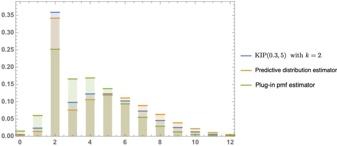
In case (b), $n=200$ , $k=2$ , $n_{k}=75$ , and $\bar{x}=3.81$ . Table 3 shows the pmf and the expected frequencies (rounded to nearest integers) of Bayes predictive distributions (corresponding to Theorem 1 [ii]) and the plug-in predictive distributions corresponding to mle’s $\hat{p}=0.13$ and $\hat{\lambda}=4.08158$ (Bayes and mle of parameters are equal, i.e., $\hat{p}_{\pi}=0.13$ and $\hat{\lambda}_{\pi}=4.08$ ).

Table 3

The Bayes and plug-in predictive distributions for future observation from $\operatorname{KIP}(0.3,5)$ , with $k=2$ and related expected frequencies

$y$	0	1	2	3	4	5	6	7	8	9	10	11	12
$\hat{q}_{\pi}(y;x)$	0.003	0.014	0.342	0.076	0.106	0.119	0.111	0.089	0.063	0.0390	0.022	0.011	0.005
Frequency of $\hat{q}_{\pi}(y;x)$	1	3	68	15	21	24	22	18	13	8	4	2	1
$\hat{q}_{\text{plug}}(y;x)$	0.015	0.060	0.252	0.166	0.169	0.138	0.094	0.055	0.029	0.0127	0.005	0.002	0.002
Frequency of $\hat{q}_{\text{plug}}(y;x)$	3	12	50	33	34	28	19	11	6	3	1	0	0

The KL loss (divergence) in Eq. (19) $\textit{KL}(\hat{q},q_{\pi})=0.009$ and $\textit{KL}(\hat{q}_{\text{plug}},q)=0.04$ , where $q(\cdot)$ , is our actual underlying distribution $\operatorname{KIP}(0.3,5)$ , with $k=2$ .

Figure 1 corresponds to Table 3.

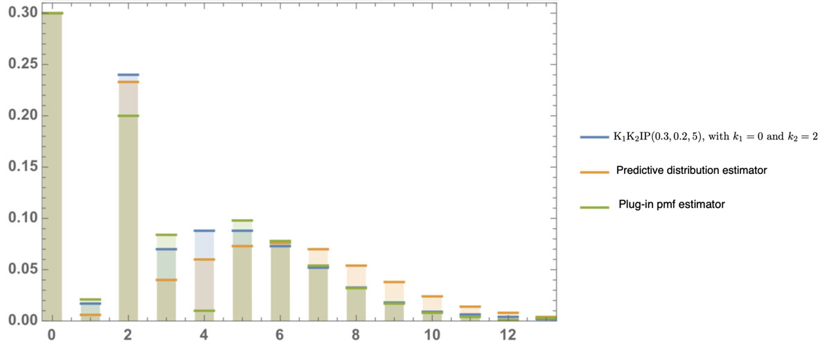
In case (c), $n=200$ , $k_{1}=0$ , $k_{2}=2$ , $n_{k_{1}}=60$ , $n_{k_{2}}=50$ , and $\bar{x}=2.99$ . The mle’s of the parameters are $\hat{p}_{1}=0.295$ , $\hat{p}_{2}=0.146$ and $\hat{\lambda}=4.831$ , and the Bayes estimators under squared error loss are $\hat{p}_{1\pi}=2.99$ , $\hat{p}_{2\pi}=0.215$ and $\hat{\lambda}_{\pi}=6.29$ . Table 4 and Fig. 2 show the Bayes and plug-in pmf estimators based on the mle’s.

Table 4

The Bayes and plug-in pmf estimators for future observation $y$ from $\operatorname{K_{1}K_{2}IP}(0.3,0.2,5)$ and related expected frequencies

$y$	0	1	2	3	4	5	6	7	8	9	10	11	12	13
$\hat{q}_{\pi}(y;x)$	0.3	0.006	0.233	0.040	0.06	0.073	0.076	0.070	0.054	0.038	0.024	0.014	0.008	0.004
Frequency of $\hat{q}_{\pi}(y;x)$	60	1	47	8	11	14	15	14	11	8	5	3	2	1
$\hat{q}_{\text{plug}}(y;x)$	0.3	0.021	0.200	0.084	0.10	0.098	0.078	0.054	0.032	0.017	0.008	0.004	0.003	0.001
Frequency of $\hat{q}_{\text{plug}}(y;x)$	60	4	40	17	20	19	16	11	6	3	2	1	1	0

Figure 1.

The pmf’s of the underlying $\operatorname{KIP(0.3,5)}$ distribution with $k=2$ , along with the Bayes and plug-in estimators related to Table 3.

Figure 2.

The pmf’s of the underlying $\operatorname{K_{1}K_{2}IP}(0.3,0.2,5)$ distribution with $k_{1}=0$ and $k_{2}=2$ , along with the Bayes and plug-in pmf estimators related to Table 4.

The KL loss (divergence) $\textit{KL}(\hat{q},q_{\pi})=0.02$ and $\textit{KL}(\hat{q}_{\text{plug}},q)=0.003$ , where $q(\cdot)$ , is our actual underlying distribution $\operatorname{KIP}(0.3,0.2,5)$ , with $k_{1}=0$ and $k_{2}=2$ .

5. Real examples

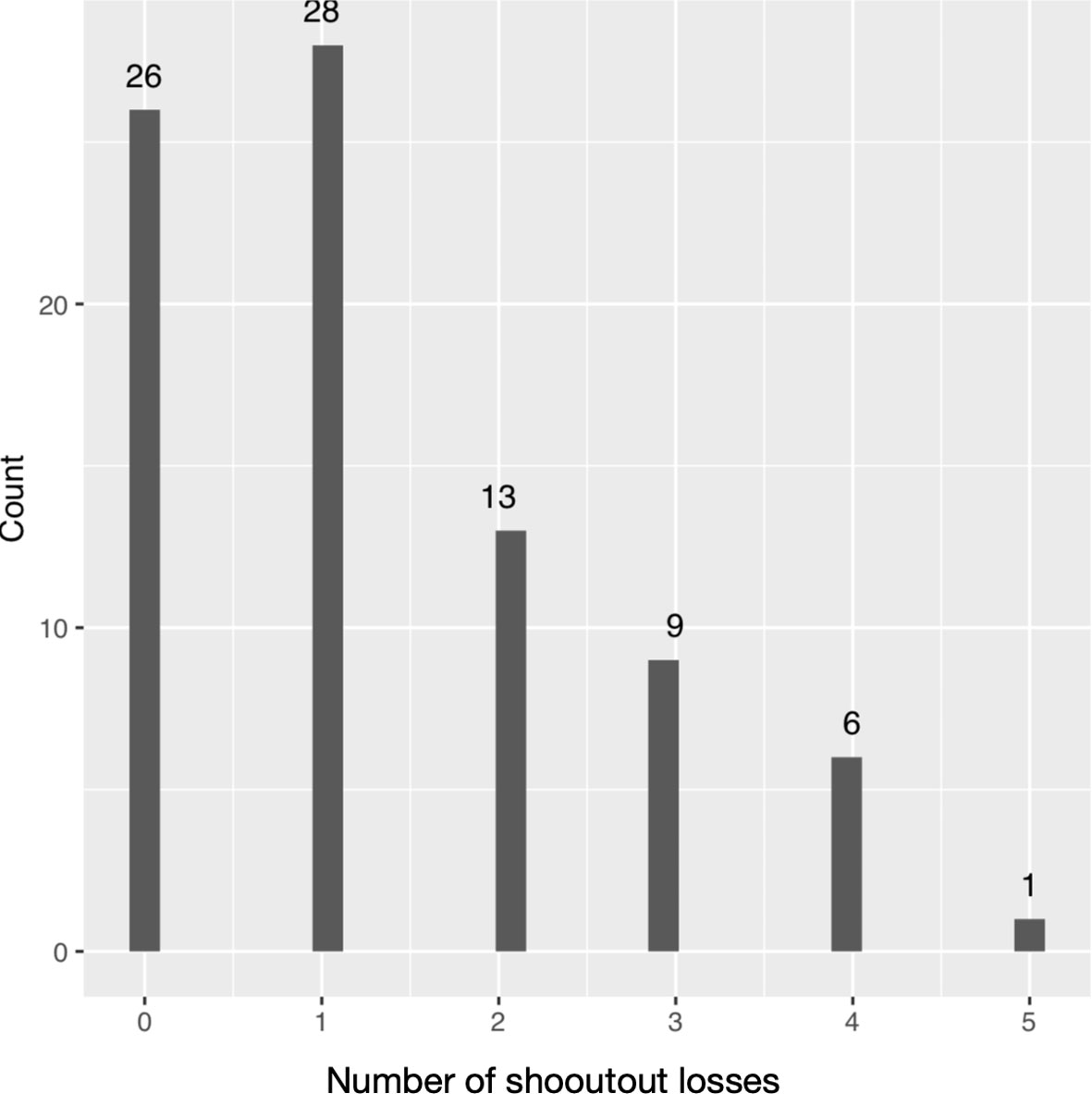
We use the number of shootout losses1 in the NHL for the season 2017/18 (see Fig. 3), and this data is available at http://www.hockeyabstract.com/testimonials/nhlgoalies2017-18www.hockeyabstract.com. The existence of excess zeros and ones in the dataset violate the Poisson assumption, thus making the $\operatorname{K_{1}K_{2}IP}$ model with $k_{1}=0$ and $k_{2}=1$ a perfect model.

Figure 3.

Number of shootout losses in the NHL’s 2017/18 season.

Applying Remark 1 gives $\hat{p}_{1}=0.219$ , $\hat{p}_{2}=0.147$ and $\hat{\lambda}=1.797$ . Likewise, using Remark 2 gives $\hat{p}_{1\pi}=0.297$ , $\hat{p}_{2\pi}=0.284$ and $\hat{\lambda}_{\pi}=3.309$ .

Below, the pmf’s of the Bayes predictive distribution $\hat{q}_{\pi}(y;x)$ under KL loss function and Jeffreys prior, along with plug-in pmf estimators based on substituting the unknown parameters by mle $\hat{q}_{\text{plug, m}}(y;x)$ and Bayes estimator of parameters (under squared error loss function) $\hat{q}_{\text{plug, b}}(y;x)$ are given, respectively.

$\displaystyle\hat{q}_{\pi}(y;x)$ $\displaystyle=\begin{cases}{0.297}&\text{if }y=0\\ {0.337}&\text{if }y=1\\ {\displaystyle\frac{\sum\limits_{j=0}^{26}\sum\limits_{l=0}^{28}\binom{26}{j}% \binom{28}{l}(84\!-\!j\!-\!l)^{-138.475+l-y}D(l\!+\!1,j\!+\!1,85\!-\!j\!-\!l)% \Gamma(138.475\!-\!l\!+\!y)}{y!\sum\limits_{j=0}^{n_{k_{1}}}\sum\limits_{l=0}^% {n_{k_{2}}}\binom{n_{k_{1}}}{j}\binom{n_{k_{2}}}{l}(83\!-\!j\!-\!l)^{-138.475% \!+\!l}D(l\!+\!1,j\!+\!1,84\!-\!j\!-\!l)\Gamma(138.475-l)}}&\text{if }y\in% \mathbb{N}\setminus\{1,2\},\end{cases}$ (27) $\displaystyle\hat{q}_{\text{plug, m}}(y;x)=\begin{cases}{0.324}&\text{if }y=0% \\ {0.316}&\text{if }y=1\\ {0.105}{\displaystyle\frac{1.798^{y}}{y!}}&\text{if }y\in\mathbb{N}\setminus\{% 1,2\},\end{cases}\quad\hat{q}_{\text{plug, b}}(y;x)=\begin{cases}{0.312}&\text% {if }y=0\\ {0.34}&\text{if }y=1\\ {0.015}{\displaystyle\frac{3.309^{y}}{y!}}&\text{if }y\in\mathbb{N}\setminus\{% 1,2\}.\end{cases}$ (28)

Table 5 shows the expected frequencies of the Bayes predictive distribution of future number of shootout losses $y$ based on Eqs (5) and (28).

Table 5

The frequency of data as well as the corresponding frequencies of Bayes and plug-in pmf estimators, based on mle and the Bayes estimator of the parameters for future number of shootout losses $y$

$y$	0	1	2	3	4	5	6	7	8	9
Data	26	28	13	9	6	1	0	0	0	0
Frequency of $\hat{q}_{\pi}(y;x)$	25	28	7	7	6	4	2	2	1	1
Frequency of $\hat{q}_{\text{plug, m}}(y;x)$	27	26	14	8	5	2	1	0	0	0
Frequency of $\hat{q}_{\text{plug, b}}(y;x)$	26	28	7	8	6	4	3	1	0	0

In this example, in order to make a comparison and show the performance of Bayes predictive distribution and the pmf estimators, one can render the Pearson goodness-of-fit test which gives the corresponding $p$ -values of 0.940, 0.940 and 0.683, for the Bayes predictive distribution $\hat{q}_{\pi}(y;x)$ , the plug-in pmf estimator based on the mle $\hat{q}_{\text{plug, m}}(y;x)$ and the plug-in pmf estimator based on the Bayes estimator of unknown parameters the $\hat{q}_{\text{plug, b}}(y;x)$ , respectively.

One can conclude that the plug-in pmf estimators based on the mle demonstrate the best performance relative to Bayes predictive distributions. To the authors’ best knowledge, for the most of continuous distributions such as normal and gamma distributions under the KL loss function (see for instance L’Moudden et al., 2017; Marchand & Sadeghkhani, 2018), the Bayes predictive density estimators outperform to the plug-in density estimators under the KL loss function. But for the discrete distributions, more specifically $\operatorname{ZIP}$ , $\operatorname{KIP}$ and $\operatorname{K_{1}K_{2}IP}$ models we do not have such dominance results. However, based on the obtained $p$ -values, the Bayes predictive distribution along with the plug-in pmf estimator fit perfectly to the data in the number if shootout losses’ example.

6. Conclusions

In summation, we have developed a model for analyzing count data with multiple inflated values that can not be modelled using typical Poisson distribution. Furthermore, we obtained the Bayes predictive distribution as well as plug-in pmf estimator for the future observation from the (a) $\operatorname{ZIP}$ model (Table 2), (b) $\operatorname{KIP}$ model (Table 3) and (c) $\operatorname{K_{1}K_{2}IP}$ model (Table 4). We also illustrated the pmf’s of the Bayes predictive distributions along with the plug-in pmf estimators in order to make comparison to the actual frequencies based on simulations from a $\operatorname{KIP}$ and $\operatorname{K_{1}K_{2}IP}$ models respectively in Figs 1 and 2.

We compared the performance of the obtained pmf estimators via simulation studies and as an application, we estimated the future pmf of the number of shootout losses using data from the NHL’s 2017/18 season. Our results confirm that the proposed pmf estimators fit perfectly to real pmfs based on the Pearson goodness-of-fit test.

Footnotes

Shootout is a method of determining a winner in hockey matches that would have otherwise been drawn or tied.

Acknowledgments

Abdolnasser Sadeghkhani acknowledges the ITAM and Asociación Mexicana de Cultura, A.C. for supporting this paper. S. Ejaz Ahmed acknowledges the Natural Sciences and the Engineering Research Council of Canada, and the Ontario Centre of Excellence for supporting this research. The authors are grateful to the editor and the anonymous reviewer for their valuable comments and helpful suggestions.

References

Corcuera

J. M.

, & Giummolè

(1999). A generalized Bayes rule for prediction. Scandinavian Journal of Statistics, 26(2), 265-279.

Ghosh

S. K.

Mukhopadhyay

, & Lu

J. C. J.

(2006). Bayesian analysis of zero-inflated regression models. Journal of Statistical Planning and Inference, 136(4), 1360-1375.

Komaki

(2004). Simultaneous prediction of independent Poisson observables. The Annals of Statistics, 32(4), 1744-1769.

Lambert

(1992). Zero-inflated Poisson regression, with an application to defects in manufacturing. Technometrics, 34(1), 1-14.

Lin

T. H.

, & Tsai

M. H.

(2013). Modeling health survey data with excessive zero and K responses. Statistics in Medicine, 32(9), 1572-1583.

L’Moudden

Marchand

É.

Kortbi

, & Strawderman

W. E.

(2017). On predictive density estimation for Gamma models with parametric constraints. Journal of Statistical Planning and Inference, 185, 56-68.

Mouatassim

, & Ezzahid

E. H.

(2012). Poisson regression and zero-inflated Poisson regression: application to private health insurance data. European Actuarial Journal, 2(2), 187-204.

Mullahy

(1986). Specification and testing of some modified count data models. Journal of Econometrics, 33(3), 341-365.

Marchand

É.

, & Sadeghkhani

(2018). On predictive density estimation with additional information. Electronic Journal of Statistics, 12(2), 4209-4238.

10.

Unhapipat

Tiensuwan

, & Pal

(2018). Bayesian predictive inference for zero-inflated Poisson (ZIP) distribution with applications. American Journal of Mathematical and Management Sciences, 37(1), 66-79.

11.

Yip

K. C.

, & Yau

K. K.

(2005). On modeling claim frequency data in general insurance with extra zeros. Insurance: Mathematics and Economics, 36(2), 153-163.