In this paper we revisit some issues related to the use of the Box-Cox transformation in censored and truncated regression models, which have been overlooked by the econometric and statistical literature. We first analyze the shape of the density function of the random variable which, rescaled by a Box-Cox transformation, leads to a normal random variable. Then, we identify the value ranges of the Box-Cox scale parameter for which a regular expectation of the derived random variable does not exist. This result calls for an extension of the concept of expectation, which can be computed regardless of the value of the scale parameter. For this purpose, we extend the concept of mean of a rescaled series of observations to the case of a random variable. Finally, we run estimates of censored and truncated Box-Cox standard Tobit models to determine the range of the scale parameter most relevant for empirical demand analyzes. These estimates highlight significant deviations from the assumption of normality of the dependent variable towards highly right skewed and leptokurtic distributions with no expectation.
In specifying parametric censored or truncated models, econometricians make an extensive use of normality assumption to model random disturbances. This assumption allows easily deriving the analytical form of the model likelihood function in order to estimate consistently and efficiently the model parameters by means of the maximum likelihood method. Unfortunately, contrary to the classical regression model which estimation is robust with respect to deviations from normality assumption of disturbances, the maximum likelihood estimation of censored or truncated regression models becomes inconsistent under non normality of disturbances.
To deal with this potential error of specification, two options are open, namely to devise robust estimation methods providing consistent estimates even in the presence of deviations with respect to the normality assumption, or to use a transformation of the non normal dependent variable to rescale it in order to turn its distribution into a normal one. In particular, to turn skewed distributions into symmetric normal-like distributions, the Box-Cox (1964) monotonic function with a free value scale parameter has been extensively applied in regression analysis of strictly positive dependent variables, as it provides a flexible family of scale transformations including linear, logarithmic and inverse scales as special cases. At a lesser extent, the Box-Cox transformation has also been used in censored or truncated regression models, notably by Poirier (1978), Lankford and Wyckoff (1991), Yen (1993), Jones and Yen (2000), Chaze (2005). In particular, to account for negative values of the dependent variable in Box-Cox Tobit models, Lankford and Wyckoff (1991) and Chaze (2005) uses a two parameter Box-Cox function which translates the lower truncation bound of the dependent variable to a negative value by adding a translation parameter to this variable in the Box-Cox function.
Empirical evidence provided by Box-Cox regression estimates seems to show that scale parameter estimates are ranging from somewhat below 0 to somewhat above 1 (Davidson & MacKinnon, 2004). But such estimates, based on classical regression assumptions, may not be relevant for Box-Cox censored and truncated regression models. On the other end, for these models such empirical evidence, based on the use of individual survey data is still not well documented. This issue deserves to be inquired to see at what extent scale parameter estimates range between 0 and 1 as, for these values, the distribution of the dependent variable is highly skewed and leptokurtic leading to an infinite expectation. This result, overlooked by the econometric and statistical literature, because mentioned in a footnote of Poirier and Melino (1978) with no formal proof, asks for reconsidering the theoretical magnitudes conventionally used for forecasting purposes and marginal effect measurement, which are nonsense when computed numerically on ground of a divergent integral formula, as made in Taylor (1986), Lankford and Wyckoff (1991) and Chaze (2005), in particular.
For sake of clarity, it is worthwhile mentioning that Box-Cox transformation has been extensively used in many fields of econometric and statistical analysis. Notably, it has been used to specify families of flexible functional forms for modeling the responses of dependent variables to changes of their explanatory variables, the flexibility of the functional form being required by the lack of a priori information provided by theory (economic or other) on the shape of the functional form. An early example of such procedure in applied econometrics is given by the use of a generalized Box-Cox cost function for modeling the interrelated demands for factors of production of an industry by Berndt and Khaled (1979), later extended by incorporating a more traditional constant elasticity of substitution cost function by Tishler and Lipovetsky (1996, 2000). This approach leads to a system of factor demands or cost shares equations where only the explanatory variables are rescaled according to a one parameter Box-Cox transformation. Hence, the empirical implementation of this model may be carried out using a classical system of nonlinear seemingly unrelated regressions. Less known is the use of the Box-Cox transformation to specify families of flexible statistical models for discrete response dependent variables, as proposed by Lipovetsky and Conklin (2000) to generalize the logistic and algebraic binary response models. From this perspective, our paper deals with a two parameters Box-Cox generalization of the censored and truncated standard Tobit model as defined in chapter 10.2 of Amemiya (1985).
On this basis, this paper intends to first carefully analyze (Section 2) the shape of what we shall call a Box-Cox normal distribution, namely the distribution of a random variable which transformation according to a Box-Cox function leads to a normal-like distribution. Our analysis complement and thorough that of Freeman and Morrades (2006), which calls the Box-Cox normal distribution: the power-normal distribution. We prefer our denomination to avoid confusion with a special case of beta distribution called “power-function distribution” (Johnson & Kotz, 1970). Then (Section 3), we identify the value ranges of the Box-Cox scale parameter for which the derived distribution does not have a regular expectation. To tackle the forecasting and marginal effect measurement problems within a Box-Cox normal regression model in a unified framework (with respect to the scale parameter values), we extend (Section 4) the concept of expectation by relating it to the transformation to normality used. This generalization of the expectation of a random variable exists for every scale parameter value of the Box-Cox transformation. Finally, we present (Section 5) econometric estimates of censored and truncated Box-Cox standard Tobit models with family expenditure survey data conducted on a large range of goods to determine the range of the Box-Cox scale parameter most relevant for empirical demand analyzes. These estimates highlight significant deviations from the assumption of normality of the dependent variable towards highly right skewed and leptokurtic distributions with no expectation. This asks for developing alternatives to the concept of expectation to tackle forecasting and marginal effect measurement issues.
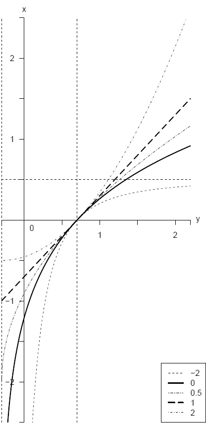
The Box-Cox transformation for different values of and .
The typical shapes of a Box-Cox normal distribution
The use of transformations to rescale a non normal variable into a normal one goes back to Edgeworth and was termed by him the Method of Translation (Johnson, 1949). Despite its dominant role in probability and theoretical statistics, it is obvious that normal distribution cannot provide an adequate representation of the vast majority of empirical distributions encountered in the real world. The most frequent departure from normality in the representation of empirical data is that referred to as skewness. The intent of the Box-Cox transformation is precisely to provide a trick to find, within a family of transformations, the one which best translate a skewed distribution into a normal-like distribution. The effectiveness of the Box-Cox transformation relies on the wide range of transformations it includes, which allows symmetrizing almost any degree of skewness, from the mildest to the heaviest, by selecting the value of a single scale parameter. Surprisingly, we found no study in the econometric and statistical literature analyzing the shape of a Box-Cox normal distribution according to the whole value range of its scale parameter, despite the importance that represents this knowledge to assess the empirical relevance of a scale parameter estimate. It is the purpose of this section to fill this gap.
Using the general two parameter transformation proposed by Box and Cox (1964):
we define a Box-Cox normal variable as the random variable leading to a normal random variable , with expected value and standard deviation , once transformed by Eq. (1), namely such that:
where stands for a standard normal variable. Parameter is termed a location parameter as it sets a lower bound, equal to , to the domain where the transformation Eq. (1) holds. Parameter is termed a scale parameter as it characterizes the degree of rescaling implemented by the Box-Cox transformation on variable . This transformation is strictly increasing and linear for , strictly convex for , and strictly concave for , with a vertical left-asymptote at when , and a ceiling asymptote at when , as shown by Fig. 1. Note also, that convexity increases with towards the limiting case of an upward right angle curve at and , reached when . Conversely, concavity increases towards the limiting case of a downward right angle curve at and when decreases towards .
The inverse Box-Cox transformation is written as:
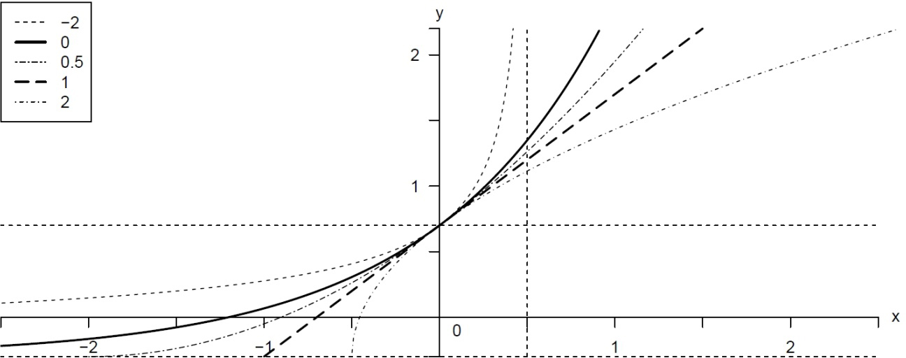
As shown by Fig. 2, the reciprocal of the Box-Cox function is strictly increasing and linear for , but strictly concave for , and strictly convex for , with a floor asymptote at when , and a vertical right-asymptote at when . Concavity increases with to reach the limiting case of a downward right angle curve at and when . Conversely, convexity increases towards the limiting case of an upward right angle curve at and when decreases towards .
The inverse Box-Cox function is defined over an unbounded range of real values only when , while for it is lower bounded by when , and upper bounded by when . Therefore, to be compatible with this domain of definition, the normal variable must be left-truncated at when , and right-truncated at when . This implies the standard normal variable in Eq. (2) shall be replaced by a truncated standard normal variable at the boundaries of the interval , which can be written in general terms as:
and
The inverse Box-Cox transformation for different values of and .
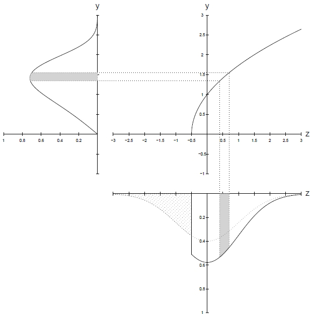
Box-Cox normal density function generated by a Box-Cox transformation with .
To analyze the profile of the probability density function of a Box-Cox normal variable, we perform the change of variable:
where denotes the truncated standard normal variable at the boundaries of interval , which density function is written as , with standing for the density function of the standard normal variable , and
with the distribution function of . Given the Jacobian of this transformation:
the density function of may be written as:
The way the Box-Cox transformation generates the profile of the density function of from that of can be illustrated by considering the “standard” case where , and (the more general case of transformation Eq. (2) will be contemplated later). To this end, we use the diagrams of Figs 3–5, inspired by Johnson (1949), representing for some outstanding values of the effect of distortion, generated by the inverse Box-Cox transformation of the -scale, on the distribution of . The shaded columns under the two density functions represent the equal probabilities of observing values of and within the corresponding small intervals and , related by , with the Jacobian of the Box-Cox transformation. Accordingly, the contraction of due to the Box-Cox transformation, implying a local amplification of the density function of , is greater where has a high value than where its value is smaller. More precisely, magnifies or reduces the value of the density function of , at the point , depending on whether or , respectively.
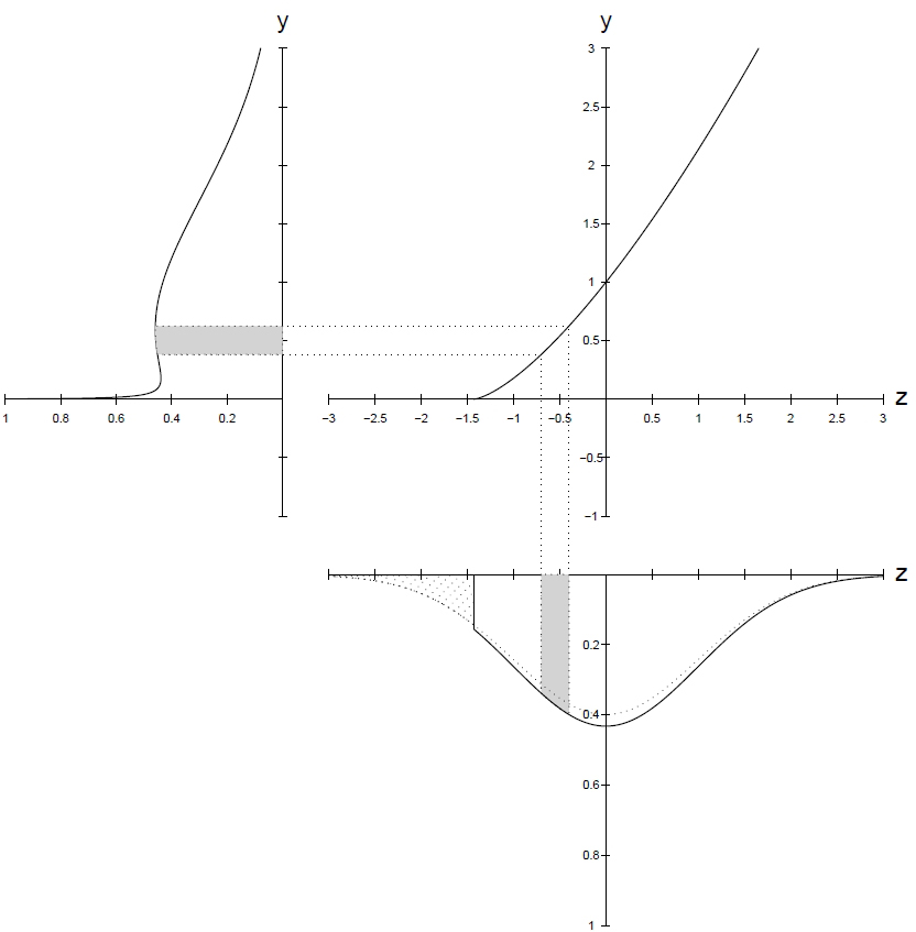
Box-Cox normal density function generated by a Box-Cox transformation with .
Box-Cox normal density function generated by a Box-Cox transformation with .
Therefore, according to the values of , many qualitatively different shapes of the density function of may be evidenced.
When , whatever the value of . Hence, the shape of the density function of is the same as that of , namely a left truncated standard normal distribution at with a mode at .
When , is an unbounded increasing function of taking value 0 at and value 1 at , while the density function of at holds finite. Hence, the density function of starts from zero and shifts the mode beyond at the value:
which is the positive solution of the following quadratic equation (with respect to the unknown obtained by equating to zero the derivative of the density function of :
This mode is an increasing function of , up to a maximum reached at ; then it decreases towards the limit value of when . Indeed, as illustrated by Fig. 3, for increasing values of since , the left truncation of increases towards 0, as well as the concentration of the probability density of around 0. Simultaneously, the concavity of the inverse Box-Cox transformation increases, since the linear case up to the case of a downward square curve with an angular point at and , when . This generates an increased concentration and symmetry of the density function of around its mode until the collapse of the entire probability mass at , when .
When , is a decreasing function of , from at to 0 when , taking value 1 at , while the density function of at holds finite. Therefore, contrary to the previous case, the density function of becomes unbounded at . Indeed, as illustrated by Fig. 4, the convexity of the inverse Box-Cox transformation increases, from the linear case up to the exponential case, for decreasing values of from to . This generates a concentration of the density function of towards 0, for , and a thickening of the density function towards , for . Despite this overall reverse J-shaped profile, the density function has still a local mode preceded by a local antimode, due to the decrease towards of the left truncation of , when . Indeed, for Eq. (11) has two positive roots, namely:
which correspond to a local minimum and a local maximum of the density function of . For , the local antimode is given by and the local mode by , as . The interpretation of roots Eq. (12) is reversed when . For , these two roots coalesce into a single one, corresponding to an horizontal inflexion point.
When , the density of is that of the well-known lognormal distribution, taking value 0 at , which corresponds to the limit of the local antimode when , and with a mode at . The value of the standard lognormal density function at the origin can be easily computed as the limit, for , of the lognormal density function written as:
Finally, when , is still a decreasing function of , taking an infinite value at , but this time the density function of at tends to 0, leading to an indeterminate product of the form . To solve this indetermination, we apply L’Hospital’s rule to the density of rewritten has the ratio of to . Computing the ratio of the derivatives of these two terms leads to:
Hence, for negative values of the density function of is unimodal right skewed, with a mode given by the positive solution Eq. (10) of Eq. (11). Written as a function of the absolute value of , , this mode may be expressed as:
and turns out to be an increasing function of , from , up to when . Furthermore, as the Jacobian’s values for increase with towards and those for decrease with towards , the concentration of the density function around its mode increases with the value of , until the collapse of the entire probability mass at , when , where the Jacobian is equal to . Indeed, as illustrated by Fig. 5, for decreasing values of since , the right truncation of decreases towards 0, while the concentration of the probability density of increases around 0. Simultaneously, the convexity of the inverse Box-Cox transformation increases, since the exponential case up to the case of an upward square curve with an angular point at and , when . This generates an increased concentration and asymmetry of the density function of around its mode until the collapse of the entire probability mass at , when .
In summary:
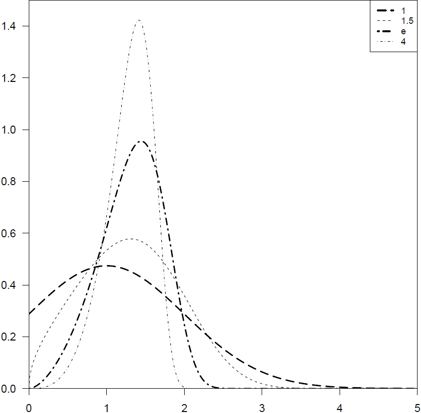
For , the density functions of is that of a unimodal left skewed distribution which concentration and symmetry around increase with , from the case of a distribution left truncated at 0, when , to the limiting case of a degenerate distribution at when .
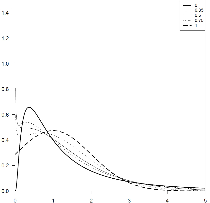
For , the density functions of is J-shaped, with a local antimode followed by a local mode, coalescing into an inflexion point with zero derivative when , and tending to 0 and , respectively, when .
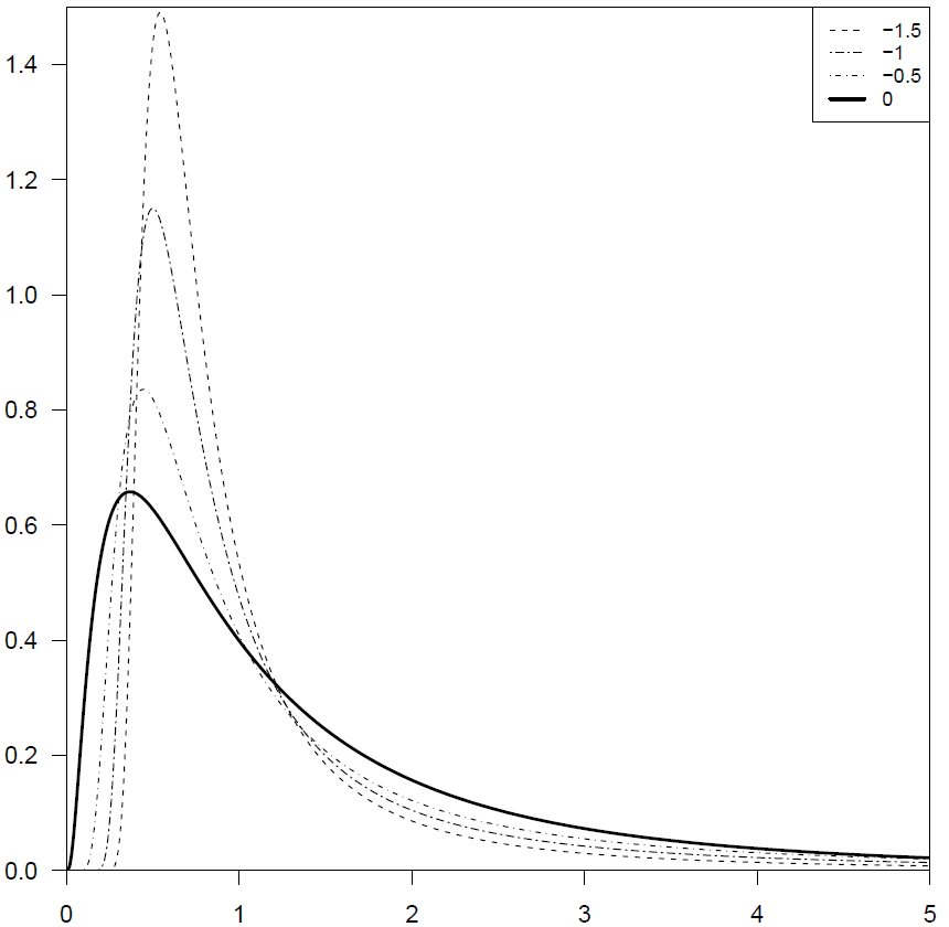
For , the density function of is that of a unimodal left skewed distribution which concentration and skewness around increase, when decreases, towards the limiting case of a degenerate distribution at when .
Shapes of the standard Box-Cox normal density function for .
Shapes of the standard Box-Cox normal density function for .
Shapes of the standard Box-Cox normal density function for .
In the general case of Box-Cox transformation Eq. (2), where density function of is written as:
equating to zero the derivative of this function leads to the following quadratic equation with respect to the unknown :
and accordingly to the following two roots with respect to :
Contrary to the possible roots of Eq. (11), which are all real numbers, the roots of Eq. (16) may be imaginary numbers, meaning that the density function Eq. (15) may not have a modal value (but may have an inflexion point). This happens when the discriminant of Eq. (16), , is negative, which is only possible for and . Conversely, when , roots of Eq. (17) are real and distinct, which corresponds to the presence of a local mode preceded by a local antimode that coalesce into an horizontal inflexion point, at , when .
For or , implying that only one of the two real roots of Eq. (16) is positive. Consequently, the density function Eq. (15) has a single global mode at .
The expectation of a Box-Cox normal distribution
Expectation is a key concept of probabilistic regression models, as it represents the causal model by which a random dependent variable is related to a set of explanatory variables. Therefore, before using these models, we must ensure of the existence of the expected value of the dependent variable, conditional to the vector of explanatory variables. In this section, we prove that an expectation for the Box-Cox normal distribution exists only for some scale parameter ranges of the Box-Cox transformation.
The mathematical expectation of the Box-Cox normal distribution Eq. (9) is defined by the following improper Riemann integral: . We remind that a Riemann integral is said to be improper if it doesn’t comply with the two basic assumptions of a Riemann integral , namely that the integration interval is finite and the integrated function is bounded over this interval.
Under the change of variable Eq. (2), this integral can be reformulated as follows, according to the values of the scale parameter .
For :
For :
For :
All these expectations are defined as limits of Riemann integrals either because the integration interval is not finite, which is the case for all the three integrals, or because the integrated function is not bounded over the integration interval, which is the case for integral Eq. (20) at .
The existence of improper Riemann integrals in expectation Eq. (19) is trivial, because it is the well known expectation of a lognormal random variable, which can be easily computed using the change of variable , leading to:
To prove the existence of improper Riemann integral in expectation Eq. (18), we use the property of dominance of function by , when , illustrated by Fig. 2: for every . According to this property, we can write the inequality:
which proves the existence of the left term of the inequality by the finite positive value of its right term.
To analyze the existence of improper Riemann integrals in expectation Eq. (20), we first observe that for , the inverse Box-Cox function is dominated by for all , as it is a positive strictly increasing function, taking value when . Therefore, for the first improper Riemann integral of Eq. (20) we can write the inequality:
which proves the existence of its left term by the finite positive value of its right term.
For the second improper Riemann integral of Eq. (20), we write two similar inequalities to lower and upper bound the integral value:
where:
Therefore, the second improper Riemann integral of Eq. (20) will converge if its upper bound will converge, and diverge if its lower bound will diverge. Now, for , the computation of these bounds gives:
and for :
Therefore, we conclude that expectation Eq. (20) does not exist for .
The -expectation of a Box-Cox normal distribution
An intuitive alternative to the expectation of the distribution of , computable for every scale parameter value of the Box-Cox transformation, is represented by the median of , as suggested by Carroll and Ruppert (1981). In this paper we explore another alternative to the expectation of a Box-Cox normal variable when the value of the scale parameter prevents its calculation, by relying on the concept of -mean of a series of observations of a variable , where denotes a monotonic transformation of . More precisely, a -mean is defined as the value of , denoted by , that rescaled by the transformation equals the arithmetic mean of the observations of rescaled by the same transformation. This leads to the following computational formula:
with the inverse of the transformation. This formula generalizes: the arithmetic mean, as it provides the arithmetic mean, when ; the geometric mean, when ; the harmonic mean, when ; the quadratic mean, when ; and so on.
A natural extension of this concept to the case of a random variable , consists in replacing in this formula the arithmetic mean of the transformed observations of , by the expectation of random variable rescaled by the transformation. This extension provides a generalization of , that exists for a Box-Cox normal distribution regardless of the value of scale parameter . We shall name it a -expectation and denote it by .
The -expectation of the Box-Cox normal distribution is defined by the following integral:
with defined by the family of functions Eq. (1) and by the family of functions Eq. (3). Under the change of variable Eq. (2), can be reformulated and computed as follows, according to the values of the scale parameter .
For :
For :
For :
By inserting these results into the inverse Box-Cox transformation Eq. (3), we finally obtain the following expressions of the -expectation.
For :
For :
For :
Empirical evidence with a Box-Cox standard Tobit model
In order to determine empirical estimates of the Box-Cox scale parameter, we use two surveys conducted by the Bureau of Labour Statistics of the U.S. Department of Labour. The first survey, called “Dairy Survey”, collects data from 10,351 households on frequently purchased goods, especially food, on a two weeks basis. The second survey, called “Interview Survey”, collects data from 25,813 households on all expenditure, on a quarterly basis. The micro-data files are publicly available on the website of the Bureau of Labour Statistics, and may be downloaded and used without permission.
For each item of expenditure listed in Tables 1 and 2, we specify a Box-Cox standard Tobit model of the form:
where represents the observed level of the dependent variable, the latent level of the dependent variable, a column-vector of explanatory variables, and a column-vector of impact coefficients of the explanatory variables on the continuous latent dependent variable.
The dependent variable is defined as the household expenditure divided the number of the household’s consumption units, computed according to the OECD definition, namely: 1 unit, for the first adult aged 18 years or over; 0.7 units, for the other adults aged 18 years or over; 0.5 units, for persons aged fewer than 18 years. According to a suggestion due to Box and Cox (1982), we rescale this measurement of the dependent variable by dividing it by its sample geometric mean, in order to have a null sample mean of for . So defined the dependent variable as well as the location parameter are pure numbers, namely dimensionless magnitudes without an explicit unit of measurement. Indeed, the ratio of a household expenditure per consumption unit () to its sample geometric mean () can be written as a product of ratios of the same magnitude, namely:
with the sample nonzero observations of .
As explanatory variables we selected:
The logarithm of household’s net income per consumption unit, and its square;
The age of household’s reference person;
The number of years of education of household’s reference person;
A binary indicator of gender of household’s reference person (1 female, 0 otherwise);
A binary indicator of an Hispanic household’s reference person (1 Hispanic, 0 otherwise);
A binary indicator of a black household’s reference person (1 black, 0 otherwise);
A binary indicator of household’s living in a SMSA (1 yes, 0 no).
Estimates of Box-Cox standard Tobit model with samples of censored observations
[l]Expenditureitem
[c]Percentageof censoredobservations
Log-tobit model
Box-Cox tobit model
: location parameter
Score test of
: scale parameter
: location parameter
Estimate
-value
Estimate
-value
Estimate
-value
[l]Dairysurvey,sample size 10351
Cereal
46
3.73
20.28
6.09
Bakeprod
23
1.55
24.15
8.16
Beef
64
3.47
20.69
7.52
Pork
63
4.49
13.58
12.33
Othmeat
64
5.03
13.90
10.48
Poultry
63
5.37
15.98
9.94
Seafood
74
3.38
12.59
8.89
Eggs
63
23.42
5.31
10.89
Milkprod
38
5.70
11.81
18.97
Othdairy
37
2.95
17.99
12.81
Frshfrut
35
1.96
23.04
5.28
Frshveg
34
1.94
31.50
4.98
Procfrut
57
5.70
10.91
11.53
Procveg
53
3.16
15.97
7.04
Sweets
53
2.01
19.97
11.26
Nonalbev
32
1.84
22.92
9.21
Oils
61
5.93
16.20
7.52
Miscfood
19
1.14
27.09
6.17
1.06
3.65
3.94
4.79
Foodaway
21
1.05
24.64
2.58
0.17
2
1.46
6.44
Alcbev
72
2.40
13.86
4.83
Smoksupp
87
2.76
8.62
3.54
0.63
0.83
6.07
1.46
Petfood
80
2.39
12.49
5.73
Persprod
61
1.45
17.20
7.58
Persserv
89
5.38
6.83
5.49
Drugsupp
72
1.06
16.61
5.74
Houskeep
41
1.24
23.51
7.60
[l]Interviewsurvey,sample size 25813
Food
1
0.23
33.63
6.94
0.15
5.00
0.36
12.17
Alcool
63
1.56
25.22
6.33
0.31
2.30
2.57
5.58
Housing
0
0.11
26.12
6.34
0.10
6.43
0.18
13.21
Apparel
40
0.90
38.90
7.81
0.31
6.69
1.69
12.56
Transport
6
0.17
42.67
37.57
1.32
20.94
1.44
31.35
Health
23
0.67
42.68
10.82
0.37
7.68
1.42
13.15
Entertainment
14
0.45
45.48
20.1
Perscare
41
1.19
33.15
13.81
0.57
4.25
2.71
7.03
Reading
80
1.58
18.06
6.54
0.36
1.82
2.79
4.00
Education
92
0.58
12.22
9.95
0.11
3.52
0.41
9.84
Tobacco
83
4.61
14.83
5.64
Miscexp
70
0.58
27.18
7.52
0.16
4.72
0.92
11.38
Cashcont
54
0.58
34.86
4.68
0.10
4.57
0.79
14.87
Insurance
20
0.61
51.04
16.68
Shows
66
0.98
27.01
6.82
0.23
3.57
1.57
8.57
Foodaway
20
0.81
41.46
16.84
0.72
6.28
2.31
9.00
Vacations
80
1.30
18.90
1.78
0.07
1.21
1.09
6.01
Estimates of Box-Cox standard Tobit model with samples of truncated observations
[l]Expenditureitem
Number ofpositiveobservations
One parameter Box-Cox
Two parameters Box-Cox
: scale parameter
score test of
: scale parameter
: location parameter
Estimate
-value
Estimate
-value
Estimate
-value
[l]Dairysurvey,sample size 10351
Cereal
5562
0.05
3.85
1.09
Bakeprod
7945
0.07
6.19
7.85
Beef
3724
0.13
10.15
1.77
0.21
5.76
0.06
2.29
Pork
3844
0.08
4.73
1.01
0.11
2.57
0.02
0.84
Othmeat
3751
0.01
0.73
2.57
0.11
2.23
0.08
1.84
Poultry
3845
0.10
6.50
1.79
0.18
3.84
0.06
1.77
Seafood
2657
0.03
2.25
1.53
0.10
2.59
0.05
1.79
Eggs
3824
0.12
6.48
2.44
0.33
3.63
0.18
2.36
Milkprod
6450
0.07
5.66
1.84
0.16
3.73
0.07
2.70
Othdairy
6553
0.04
2.85
5.04
Frshfrut
6752
0.12
12.39
5.80
Frshveg
6856
0.09
13.75
0.89
0.07
8.01
0.01
1.39
Procfrut
4461
0.07
4.80
1.09
0.04
1.18
0.02
0.92
Procveg
4816
0.05
3.65
0.04
0.05
2.27
0
0.04
Sweets
4912
0.06
5.12
0.62
0.08
2.88
0.01
0.50
Nonalbev
7055
0.09
8.73
5.27
Oils
4006
0
0.16
1.12
0.05
1.57
0.04
1.91
Miscfood
8426
0.14
16.28
7.08
Foodaway
8154
0.18
20.83
19.73
Alcbev
2917
0.06
4.56
1.60
0.02
0.79
0.02
1.23
Smoksupp
1393
0
0.16
6.24
Petfood
2049
0
0.01
2.28
0.08
2.13
0.05
1.89
Persprod
4045
0.03
2.32
2.70
Persserv
1142
0.03
1.17
1.82
0.10
1.46
0.04
1.12
Drugsupp
2913
0.06
5.08
0.71
0.07
3.55
0.01
0.55
Houskeep
6141
0.08
12.46
3.74
0.02
0.94
0.07
3.51
[l]Interviewsurvey,sample size 25813
Food
25664
0.13
25.34
4.08
0.06
4.04
0.05
4.47
Alcool
9510
0.07
10.00
0.55
Housing
25753
0.10
30.22
3.10
0.06
3.88
0.12
8.35
Apparel
15394
0.08
18.90
3.33
Transport
24334
0.02
7.01
9.95
1.34
21.01
1.41
25.45
Health
19940
0.16
44.09
5.53
Entertainment
22224
0.05
15.19
6.71
0.18
9.85
0.21
9.38
Perscare
15140
0.02
3.53
6.11
Reading
5235
0.03
3.04
1.42
0
0.25
0.01
1.17
Education
2110
0
0.26
7.29
Tobacco
4509
0.12
11.66
0.13
Miscexp
7727
0.04
7.36
0.23
0.04
5.44
0
0.16
Cashcont
11848
0.02
4.80
0.04
0.02
3.53
0
0.02
Insurance
20608
0.13
64.36
4.03
Shows
8679
0
0.18
1.41
0.01
0.71
0
1.11
Foodaway
20647
0.07
14.63
3.15
0.03
3.05
0.02
3.23
Vacations
5131
0.09
11.24
0.47
0.07
4.37
0.01
1.25
To estimate the parameters of model Eq. (36) by the maximum likelihood method, we need to derive the probability distribution of an observation of the dependent variable .
If such an observation is censured, and therefore can take either a value or , its distribution is a discrete-continuous mixture, which assigns a probability mass to and a density function to any , with: . Note that only for .
Now, the density function is written as Eq. (9) with , while the computation of can be performed using the change of variable:
From these results we derive the following expression of the log-likelihood for a random sample of observations of a censored dependent variable :
If the observation of is truncated only values can be observed. Thus, the distribution of is that of a continuous random variable with density function given by:
with given by Eq. (40). Thus, the log-likelihood for a random sample of observations of a truncated dependent variable is written as:
Table 1 presents the results of estimating the Box-Cox standard Tobit model Eq. (36) with the full sample of censured observations (10’351 observations for the “Dairy Survey”, and 25’813 observations for the “Interview Survey”). The first part of the table presents the estimation of a lognormal Tobit model of the dependent variable. To test this assumption, we provide the score test statistics for the assumption , which is asymptotically distributed according to a standard normal random variable. The reported results show that a highly significant positive estimate of the location parameter has been obtained for all the expenditure items of both surveys, which comply with the presence in the survey data of a moderate to very high rate of censored observations. According to the values of the score statistics, the maintained assumption of log normality of the dependent variables is significantly rejected against a more skewed distribution characterized, with one exception (education), by negative values of parameter . The second part of Table 1 displays the joint maximum likelihood estimation of both parameters and , with the corresponding t-statistics. For all items for which such a joint estimate has been obtained, the results confirm the sign of parameter indicated by the score test. On the other hand, a strong negative correlation between these two parameter estimators significantly reduces their statistical significance as well as the power of the score test for the assumption .
Common sense suggests that these disappointing results stem from an inadequate consideration of the actual mechanisms generating the censored observations. Indeed, the standard Tobit model attributes the censorship of the expenditure for the purchase of a given good or service to a negative desired level of consumption of the consumer, as a consequence of an economic rational decision based on his preferences, resources and good prices. If such a mechanism may be relevant to explain the censoring of expenditures for luxury goods, as it is the case for some of the expenditure items of the “Interview Survey” (notably “shows” and “vacations”), it is hardly to be a credible explanation for the censorship of the expenditure items of the “Dairy Survey”, which specificity and duration of the survey period call for the use of other censoring mechanisms; notably Cragg (1971) good selection mechanism and Deaton and Irish (1984) infrequent purchasing mechanism. Adding these mechanisms to the standard Tobit model alters the likelihood function of a censured sample but not that of a truncated sample, when the added censoring mechanisms are independent of the standard Tobit relation. Indeed, suppose we add to the Box-Cox standard relation Eq. (36) two new censoring mechanisms modelled by two latent variables and jointly independent of , with . For this model the probability of a censored observation is given by . As the joint density function of , and is written as , the density function of a positive observation of may be expressed as follows:
For a truncated observation of , this leads to the following density function:
which corresponds to the truncated density function of the Box-Cox standard Tobit model Eq. (43).
For this reason we can expect more relevant results in estimating parameters and with the truncated samples of observations. These estimates are shown in Table 2, displaying in a first part the maximum likelihood estimates of the scale parameter , with the corresponding t-statistics, performed by assuming , and the score test statistics for this assumption as an indicator of the direction of search of a free estimate of , namely for a negative value of the score test, and for a positive value. The second part of the table displays the joint maximum likelihood estimates of parameters and , with the corresponding t-statistics, for all the expenditure items for which a positive estimate of the location parameter is expected, with two exceptions (transport and insurance of the “Interview Survey). From these estimates we can conclude that negative estimates of parameter are prevalent compared to positive estimates. For the expenditure items of the “Dairy Survey”, 13 estimates of this parameter are negative, ranging between 0.33 and 0.02, while only 4 estimates are positive, ranging between 0.02 and 0.07. For the “Interview Survey”, 5 estimates are negative, ranging between 1.34 and 0.01, 4 estimates are positive, taking values between 0.02 and 0.07, and an estimate is zero.
Conclusion
The empirical results presented in Section 5 suggest that in analyzing family expenditures for consumption goods and services at a detailed or semi-aggregate level with Box-Cox Tobit models, we must expect to be faced to significant departures from the assumption of normality of the dependent variable towards highly right skewed and leptokurtic probability distributions with no expectation. The non existence of the expectation of the dependent variable asks for reconsidering the theoretical magnitudes conventionally used for forecasting purposes and marginal effect measurement. To this end, the concept of T-expectation presented in Section 4 deserves to be experienced empirically and theoretically analyzed. Our research is continuing in this direction.
Footnotes
Acknowledgments
We thank the MASA Co-Editor-in-Chief, Prof. Stan Lipovetsky, for suggesting to benchmark our findings to former applications of the Box-Cox transformation in econometrics and in statistics.
References
1.
AmemiyaT. (1985). Advanced econometrics. Harvard University Press, Cambridge (MA).
2.
BerndtE. R., & KhaledM. (1979). Parametric productivity measurement and choice among flexible functional forms. Journal of Political Economy, 87(6), 1220-1245.
3.
BoxG., & CoxD. (1964). An analysis of transformations. Journal of the Royal Statistical Society. Series B (Methodological), 26(2), 211-252.
4.
BoxG. E. P., & CoxD. R. (1982). An analysis of transformations revisited, rebutted. Journal of the American Statistical Association, 77(377), 209-210.
5.
CarrollR. J., & RuppertD. (1981). On prediction and the power transformation family. Biometrika, 68(3), 609-615.
6.
ChazeJ. (2005). Assessing household health expenditure with box-cox censoring models. Health Economics, 14(9), 893-907.
7.
CraggJ. (1971). Some statistical models for limited dependent variables with applications for the demand for durable goods. Econometrica, 39(5), 829-844.
8.
DavidsonR., & MackinnonJ. G. (2004). Econometric theory and methods. Oxford University Press.
9.
DeatonA., & IrishM. (1984). A statistical model for zero expenditures in household budgets. Journal of Public Economics, 23, 59-80.
10.
FreemanJ., & ModarresR. (2006). Inverse box-cox: The power-normal distribution. Statistics & Probability Letters, 76(8), 764-772.
JohnsonN. L. (1949). Systems of frequency curves generated by methods of translation. Biometrika, 36(1-2), 149-176.
13.
JonesA. M., & YenS. T. (1994). A box-cox double hurdle model. The Manchester School, 68(2), 203-221.
14.
LankfordR. H., & WyckoffJ. (1991). Modeling charitable giving using a box-cox standard tobit model. The Review of Economics and Statistics, 73(3), 460-470.
15.
LipovetskyS., & ConklinM. (2000). Box-cox generalization of logistic and algebraic binary response models. International Journal of Operations and Quantitative Management, 6, 276-285.
16.
PoirierD. J. (1978). The use of the box-cox transformation in limited dependent variable models. Journal of the American Statistical Association, 73(362), 284-287.
17.
PoirierD. J., & MelinoA. (1978). A note on the interpretation of regression coefficients within a class of truncated distributions. Econometrica, 46(5), 1207-1209.
18.
TaylorJ. (1986). The retransformed mean after a fitted power transformation. Journal of the American Statistical Association, 81(393), 114-118.
19.
TishlerA., & LipovetskyS. (1997). The flexible ces-gbc family of cost functions: Derivation and application. The Review of Economics and Statistics, 79(4), 638-646.
20.
TishlerA., & LipovetskyS. (2000). A globally concave, monotone and flexible cost function: Derivation and application. Applied Stochastic Models in Business and Industry, 16(4), 279-296.
21.
YenS. T. (1993). Working wives and food away from home: The box-cox double hurdle model. American Journal of Agricultural Economics, 75(4), 884-895.