The beta and simplex regression models to explain homicides in state capitals of Brazil

Abstract

The intentional killing of one human being by its own kind is considered the worst of the crimes. Therefore, homicide prevention is a major concern for policy makers in both developing and developed countries. We propose regression modeling for the homicide rates in Brazil along with appropriately chosen distributions for these responses that are in agreement with the restriction of values to the unit interval. We adopt the beta and simplex regression models with systematic components for the mean and dispersion parameters to explain the homicide rates in 27 state capitals of Brazil from the following explanatory variables: time, Gini coefficient, municipal human development index (MHDI), illiteracy and poverty rates. We employ standard likelihood techniques, perform influence and residual analysis and calculate goodness-of-fit statistics to select the best regression to explain homicides rates in these capitals. We perform the computations in the R package. The main results suggest the following: the mean homicide rate is increasing over time; there is a negative correlation between MHDI and murder rate; the poverty has a quite small negative impact on the mean homicide rates in the beta regression. The Gini coefficient and the illiteracy and poverty rates explain the dispersion of the homicide rates.

Keywords

Beta regression homicide rate maximum likelihood simplex regression

1. Introduction

In this paper, we employ both beta and simplex regressions to explain the variability of the homicide rates in all Brazilian state capitals using data sets from three separated years (1991, 2000 and 2010). The homicide, defined here as an unlawful death deliberately inflicted on one person by another person, is considered the worst of the crimes. According to the United Nation Office on Drugs and Crime, half of all homicides occur in countries that gather 11% of the global population. There is significant variation across and within nations. For instance, in 2012, the global homicide average was estimated at 6.2 per 100,000 habitants, thus representing up to 437,000 violent deaths. Some regions, such as Central America and Southern Africa, have rates close to 25 cases per 100,000 population, while Southern and Western Europe have averages up to six times lower than the global mean. The Americas (16.3) and Africa (12.5) are significant more violent than Europe (3) and Asia (2.9). In addition to spatial dependence, the homicides dispersion also follows different longitudinal trends. For example, Eisner (2003) provided long-term homicide rates across Western Europe and showed that murder rates dramatically decreased over time. Conversely, official data from England and Wales (1967–2017) show a more complex pattern with a positive linear trend from 1960 to 1990 and an exponential increase from 1999 to 2003. After a ten years’ negative trend, homicides started to increase again in 2015.

On theoretical grounds, scholars from different disciplines try to identify which variables explain homicides variation. For the best of our knowledge, Kronh (1976) and McDonald (1976) provided pioneer cross-national comparisons on property crime from police statistics. In particular, early academic works have systematically found a positive association between socioeconomic variables and homicide rates (Loftin & Hill, 1974; Parker & Smith, 1979; Parker & Loftin, 1983). Blau and Blau (1982) and Messner (1982) reported null results regarding the poverty-homicide link. Braithwaite and Braithwaite (1980) used data from 31 countries over a 20-year period (1955–1974) to estimate the relationship between crime and income inequality. They reported that most of the variables have a strong and statistically significant correlation with homicides. The authors performed several tests, but they used to evaluating these countries the following variables: political freedom, ethnic fictionalization, gross domestic product (GDP) per capita and intersectorial income inequality. Williams (1984) employed a nonlinear model to examine the relationship between poverty levels and homicide rates for 125 statistical metropolitan areas in the United States. Gartner (1990) estimated a time-series-cross-section model using sex and age specific victimization data from 18 countries (1950–1980). According to Nivette (2011), there was a series of theoretical approaches in cross-sectional studies of crimes’ predictors. Applying meta-analysis, the author identified 10 different perspectives and most of the work are based on demographic explanatory variables.

Messner (1982) identified two measures of deprivation: absolute and relative. The first is defined as the proportion of a population below a fixed measure of well-being. The latter represents the relative dispersion of income within a specific population. According to Roberts and Willits (2015), for the relative deprivation perspective “individuals evaluate their socio-economic standing in relation to others, and develop frustration, hostility, and resentment when they realize that they have fewer resources than others”. More recently, Kelly (2000) used data from 1991 FBI Uniform Crime Reports to find that inequality has a strong impact on violent crimes, but no effect on property offenses. He also reported that poverty and police activity explain the variation of violent crime, but have little correlation with property incidents. Roberts and Willits (2015) argued that different measures of inequality may lead to mixed findings on the income inequality-homicide link. Based on data from 208 U.S. cities, they reported that all measures of inequality are positively correlated with homicide rates. Thus, their proposed mechanism between income inequality and crime relies on the concept of deprivation.

Among developing countries, Brazil has two interesting features: extreme income inequality and high crime rates, particularly homicides. According to official estimates, Brazil was responsible for 10% of world homicides in 2015 which means almost 60,000 violent deaths, see: https://www.nytimes.com/2018/08/10/world/americas/brazil-murder-rate-record.html. In 2016, the country reached a new record with more than 62,000 killings. We choose homicide rate as dependent variable because it is the most commonly employed in comparative research and has higher variability over the state capitals in Brazil. In addition, homicide has higher levels of reportability and uniformity than others types of crime, which decreases measurement error (Braithwaite & Braithwaite, 1980). Data from Organization for Economic Co-operation and Development (OECD) suggest that wealth distribution in Brazil is extremely concentrated. In fact, the Gini coefficient, which is a statistical measure of income inequality of a population, is 0.54 in Brazil, one of the highest in the world. The five richest Brazilian have the same wealth of the 52% poorest. The overall Gini index of United Kingdom is 0.35 thus representing a more equal society. In this context, Brazil is an important country to be investigated, thus representing a unique opportunity to learn how extreme income inequality relates with homicide rates.

In applied fields, outcomes of rates or proportions often arise. Few models are suitable for fitting such data. In this paper, we apply the beta and simplex regressions with varying dispersion to predict homicide rates in Brazil. The beta regression is commonly used to model continuous variables restricted to the interval $(0,1)$ (Ferrari & Cribari-Neto, 2004). However, with an additional dispersion parameter, the simplex regression based on the simplex distribution (Barndorff-Nielsen & Jørgensen, 1991) may be more robust in some cases for analysis of continuous proportional data. We employ here both regression models to explain the homicide rates for all Brazilian state capitals.

Outcomes of continuous proportions or rates arise in many applied areas including social and political sciences. Regression models for proportional data have be in widespread use in the last fifteen years or so. These regressions employ a continuous distribution for the response in the interval $(0,1)$ parameterized in terms of the mean and dispersion parameters. One important motivation for this work could center on the modeling of dispersion parameters for responses, in addition to modeling expectation functions. In the original presentations of the beta regression (Ferrari & Cribari-Neto, 2004) and simplex regression (Song & Tan, 2000), the dispersion parameter of response distributions was assumed constant across all observations. This is analogous to an assumption of homoscedasticity in normal regression. In this work, we relax this assumption, modeling both expectation and dispersion parameters as functions of explanatory variables.

The paper is organized as follows. In Section 2, we provide a summary of the beta and simplex regressions. We employ the likelihood function to measure the adequacy of the fitted regressions to the homicide rates. The parameter estimates are those values that maximize the log-likelihood. There are simple computer programs to fit most common regression models. Also, we present some diagnostic measures and residuals. In Section 3, we give details of the homicide data collected in the state capitals of Brazil and discuss the fitted of two regressions to these data. Finally, some concluding remarks are offered in Section 4.1.

2. The beta and simplex regression background

In this section, we present a background related to the (i) beta regression, (ii) simplex beta and (iii) diagnostic and residual analysis.

2.1 The beta regression

An important class of problems involves data in the forms of rates and proportions, such as mortality rates, infection rates of diseases, etc. So, the beta distribution is useful for modeling random experiments that produce results in the interval $(0,1)$ measured continuously. The density of a random variable $Y$ having the beta distribution with parameters $p>0$ and $q>0$ is

$\displaystyle f(y;p,q)=\frac{\Gamma(p+q)}{\Gamma(p)\Gamma(q)}y^{p-1}(1-y)^{q-1% },\quad y\in(0,1),$

where $\Gamma(\cdot)$ is the gamma function. The mean and variance of $Y$ are, respectively,

$\displaystyle\text{E}(Y)=\frac{p}{p+q}\quad\text{and}\quad\text{Var}(Y)=\frac{% pq}{(p+q)^{2}(p+q+1)}.$

We adopt the beta density implemented in the Generalized Additive Model for Location, Scale and Shape (GAMLSS) software with mean parameter $\mu$ and dispersion parameter $\sigma$ having the re-parametrization $p=\mu(1-\sigma^{2})/\sigma^{2}$ and $q=(1-\mu)(1-\sigma^{2})/\sigma^{2}$ , where $0<\mu<1$ and $0<\sigma<1$ . Under this re-parametrization, we write $Y\sim B(\mu,\sigma)$ and then the density of $Y$ has the form

$\displaystyle f(y;\mu,\sigma)=J(\mu,\sigma)y^{\frac{\mu(1-\sigma^{2})}{\sigma^% {2}}-1}(1-y)^{\frac{(1-\mu)(1-\sigma^{2})}{\sigma^{2}}},\quad y\in(0,1),$ (1)

where

$\displaystyle J(\mu,\sigma)=\frac{\Gamma\left(\frac{1-\sigma^{2}}{\sigma^{2}}% \right)}{\Gamma\left(\frac{\mu(1-\sigma^{2})}{\sigma^{2}}\right)\Gamma\left(% \frac{(1-\mu)(1-\sigma^{2})}{\sigma^{2}}\right)}.$

Here, the mean and the variance of $Y$ are $\text{E}(Y)=\mu$ and $\text{Var}(Y)=\sigma^{2}V(\mu)$ , where $V(\mu)=\mu(1-\mu)$ and $\sigma$ really works as a dispersion parameter.

Let $y=(y_{1},\ldots,y_{n})^{\top}$ be a random sample, where $y_{i}\sim B(\mu_{i},\sigma_{i}),i=1,\ldots,n$ . The systematic components for the beta regression, where both mean and dispersion vary across observations, take the forms

$\displaystyle\eta_{i}=g(\mu_{i})=\bm{x}_{i}^{\top}\bm{\beta}\quad\text{and}% \quad\rho_{i}=h(\sigma_{i})=\bm{z}_{i}^{\top}\bm{\gamma},$ (2)

where $g(\cdot)$ and $h(\cdot)$ are known one-to-one twice continuously differentiable functions, called the mean and dispersion link functions, respectively, $\eta_{i}$ and $\rho_{i}$ are the linear predictors, $\bm{x}_{i}=(x_{i1},\ldots,x_{ir})^{\top}$ is the $r$ -vector of non-stochastic independent variables and $\bm{z}_{i}=(z_{i1},\ldots,z_{is})^{\top}$ is the $s$ -vector of the dispersion explanatory variables (both associated with the $i$ th observation) and $\bm{\beta}=(\beta_{1},\ldots,\beta_{r})^{\top}$ and $\bm{\gamma}=(\gamma_{1},\ldots,\gamma_{s})^{\top}$ are the $r\times 1$ and $s\times 1$ vectors of unknown regression coefficients. It is very common to choose $\bm{z}_{i}$ as a subset of $\bm{x}_{i}$ . Let $\bm{\eta}=(\eta_{1},\ldots,\eta_{n})^{\top}$ and $\bm{\rho}=(\rho_{1},\ldots,\rho_{n})^{\top}$ be the linear predictor vectors. Moreover, we consider that the link functions $g:(0,1)\rightarrow\mathbb{R}$ and $h:(0,1)\rightarrow\mathbb{R}$ are strictly monotonic and twice differentiable. A number of different link functions can be appropriate but the logit specification $g(w)=h(w)=\log[w/(1-w)]$ is the most popular in applications.

Consider a sample $(y_{1},\bm{x}_{1}),\ldots,(y_{n},\bm{x}_{n})$ of $n$ independent observations. The log-likelihood function for the vector of parameters $\bm{\theta}=(\bm{\beta}^{\top},\bm{\gamma}^{\top})^{\top}$ for the model defined by Eq. (1) and (2) can be expressed as

$\displaystyle l(\bm{\theta})=\sum_{i=1}^{n}\log[J(\mu_{i},\sigma_{i})]+\sum_{i% =1}^{n}\log(y_{i})\left[\frac{\mu_{i}(1-\sigma_{i}^{2})}{\sigma_{i}^{2}}-1% \right]+\sum_{i=1}^{n}\log(1-y_{i})\left[\frac{(1-\mu_{i})(1-\sigma_{i}^{2})}{% \sigma_{i}^{2}}-1\right],$ (3)

where $\mu_{i}=g^{-1}(\eta_{i})$ and $\sigma_{i}=\rho^{-1}(\rho_{i})$ are known functions of $\bm{\beta}$ and $\bm{\gamma}$ defined by Eq. (2).

2.2 The simplex regression

The simplex dispersion (SD) density (Barndorff-Nielsen & Jrgensen, 1991) for a univariate continuous random variable $Y$ has the form

$\displaystyle\pi(y;\mu,\sigma^{2})=\frac{1}{\sqrt{2\pi\sigma^{2}V(y)}}\exp% \left[-\frac{{\rm d}(y;\mu)}{2\sigma^{2}}\right],y\in(0,1),$ (4)

where $\mu\in(0,1)$ is the mean parameter, $\sigma^{2}>0$ is the dispersion parameter, $V(y)=y^{3}(1-y)^{3}$ is called the variance function and

$\displaystyle{\rm d}(y;\mu)=\frac{(y-\mu)^{2}}{y(1-y)\mu^{2}(1-\mu)^{2}}$ (5)

is the unit deviance.

Let $l(y;\mu)$ be the log-likelihood for $\mu$ corresponding to one observation $y$ from Eq. (4). A simple interpretation for the unit deviance comes from the unit log-likelihood as ${\rm d}(y;\mu)=-2l(y;\mu)$ . The mean and variance of the unit deviance are $E[{\rm d}(Y;\mu)]=\sigma^{2}$ and $\text{Var}[{\rm d}(Y;\mu)]=2\sigma^{4}$ (see, for example, Song & Tan, 2000).

We denote a random variable $Y$ having a simplex distribution with mean $\mu$ and dispersion parameter $\sigma^{2}$ by $Y\sim S(\mu,\sigma^{2})$ .

Let $Y_{1},\ldots,Y_{n}$ be independent random variables such that $Y_{i}$ follows the $S(\mu_{i},\sigma_{i}^{2})$ density given by Eq. (4) (for $i=1,\ldots,n$ ). We define the simplex regression by the random component Eq. (4) and the systematic components Eq. (2) under a different mapping required for the dispersion link function, i.e., $h:(0,\infty)\rightarrow\mathbb{R}$ . The homogeneous simplex regression is determined by removing the varying dispersion effects in Eq. (2) making the variance of $Y_{i}$ depending only on the explanatory variables $x_{i}^{\prime}$ s in the means.

Let $y=(y_{1},\ldots,y_{n})^{\rm T}$ be a set of observations. Given $y$ , let $\ell=\ell(\bm{\theta})$ be the total log-likelihood function for the simplex regression given earlier in terms of $\bm{\theta}=(\bm{\beta}^{\rm T},\bm{\gamma}^{\rm T})^{\rm T}$ . The parameters in $\bm{\beta}$ and $\bm{\gamma}$ are estimated by the iteratively re-weighted least squares (IRWLS) algorithm by maximizing $\ell(\bm{\theta})$ (except for a constant term)

$\displaystyle\ell(\bm{\theta})=-\frac{1}{2}\sum_{i=1}^{n}\left[\frac{{\rm d}(y% _{i};\mu_{i})}{\sigma_{i}^{2}}-\log(\sigma_{i}^{2})\right].$ (6)

The maximization of Eqs (3) and (6) can be performed by the RS algorithm. See details in Rigby and Stasinopoulos (2005) and Stasinopoulos and Rigby (2007). All computational procedures for the simplex regression are done in GAMLSS software in R.

2.3 Influence and residual analysis

For the beta and simplex regressions defined before, the log-likelihood function of $\bm{\theta}$ is denoted by $l_{(i)}(\bm{\theta})$ . In the following, a quantity with subscript “(i)” means the original quantity with the $i$ th observation deleted. Let $\hat{\bm{\theta}}_{(i)}=(\hat{\bm{\beta}}_{(i)}^{\rm T},\hat{\bm{\gamma}}_{(i)% }^{\rm T})^{\rm T}$ be the MLE of $\bm{\theta}$ obtained from maximizing $l_{(i)}(\bm{\theta})$ . To assess the influence of the $i$ th observation on the MLEs $\hat{\bm{\theta}}=(\hat{\bm{\beta}}^{\rm T},\hat{\bm{\gamma}}^{\rm T})$ , we can compare the difference between $\hat{\bm{\theta}}_{(i)}$ and $\hat{\bm{\theta}}$ . If deletion of an observation seriously influences the estimates, more attention should be paid to that observation. Hence, if $\hat{\bm{\theta}}_{(i)}$ is far from $\hat{\bm{\theta}}$ , then the $i$ th observation can be regarded as influential. A first measure of the global influence is defined as the standardized norm of $\hat{\bm{\theta}}_{(i)}-\hat{\bm{\theta}}$ (generalized Cook distance) $GD_{i}(\bm{\theta})=(\hat{\bm{\theta}}_{(i)}-\hat{\bm{\theta}})^{\rm T}[\ddot{% \textit{L}}(\hat{\bm{\theta}})](\hat{\bm{\theta}}_{(i)}-\hat{\bm{\theta}})$ , where $\ddot{\textit{L}}(\hat{\bm{\theta}})$ is the matrix of the second-derivatives of the log-likelihood $\ell=\ell(\bm{\theta})$ evaluated at $\hat{\bm{\theta}}$ .

Another popular measure of the difference between $\hat{\bm{\theta}}_{(i)}$ and $\hat{\bm{\theta}}$ is the likelihood distance $LD_{i}(\bm{\theta})=2[l(\hat{\bm{\theta}})-l(\hat{\bm{\theta}}_{(i)})]$ .

In order to study departures from the distribution assumption as well as the presence of outlying observations, we consider the normalized randomized quantile residuals (Dunn & Smyth, 1996). These residuals are determined by $\hat{r}_{i}=\Phi^{-1}(\hat{u}_{i})$ , where $\Phi^{-1}(\cdot)$ is the inverse standard normal cumulative distribution and $\hat{u}_{i}=F(y_{i}|\hat{\bm{\theta}})$ is the estimated cdf of the beta or simplex distribution.

We also use Worm Plots (WP) of the residuals (Buuren & Fredriks, 2001) as the technique to check the adjustment quality. The general idea of these plots is to identify regions (intervals) of an explanatory variable within which the model does not fit adequately to the data. Model inadequacy is indicated when many observations lie outside the point-wise 95% confidence bands or when the points follow a systematic shape. For example, the interpretations of the shapes of the WP are: a vertical shift, a slope, a parabola or a S shape, thus indicating a misfit in the mean, variance, skewness and excess kurtosis of the residuals, respectively.

We build envelopes to enable better interpretation of the normal probability plot of the residuals. These envelopes are simulated confidence bands described by Atkinson (1985) that contain the residuals such that if the model is well-fitted, the majority of points will be randomly distributed within these bands.

3. Data

We consider the data for the 27 Brazilian state capitals in three separated years (1991, 2000 and 2010). The dependent variable is the homicide rate measured by the number of homicides in the city normalized by its total population. All variables were collected at the city level using public secondary data from DATASUS (http://datasus.saude.gov.br/ and IPEADATA http://www.ipeadata.gov.br/Default.aspx). We select the following explanatory variables: year, region, Gini index, per capita income, poverty rate, illiteracy rate and municipal human developing index (MHDI). The Gini coefficient is a statistical measure of income inequality of a population. A coefficient of zero represents perfect equality while a Gini of one suggests maximum inequality. It is 0.54 in Brazil, one of the highest in the world. In fact, the five richest Brazilian have the same wealth of the 52% poorest. The overall Gini index of United Kingdom (UK) is 0.35 thus representing a more equal society. The poverty rate is the proportion of people living below the poverty line, i.e. who lives with less than 5.5 US dollars a day. Brazil has about 40 million poor people. The illiteracy rate is the proportion of the adult population that cannot read and write simple sentences. The average illiteracy rate of 10% in Brazil represents a complex educational problem. The MHDI is the geometric mean of three normalized indices that measure the life expectation, years of education and living conditions (gross income per capita). The latest Brazil’s homicide rate is 28 homicides per 100,000 people thus placing Brazil in the top 20 countries by homicide rates. Brazil’s homicide rate is on average 32 higher than UK’s overall rate.

Brazil is divided in five regions that spread out over 27 states. The Southeast and South are the most developed regions. The North and Northeast are the poorest parts of the country, which concentrate 36% of the total population. About half of the people that live in these two regions earn less than 125 US dollars a month. The curves of homicide rates in the cities follow very different patterns. In the 2000–2010 period, Maceió more than double the homicide rate, whereas São Paulo has a big decay. In the total 20 years, João Pessoa and Salvador have more than triple homicide rates. In the South capitals, there is no decrease in the homicide rates. In the North, Northeast and South, the average homicide rates grow steadily in the whole period.

As long as regression models dealing with rates and proportions are typically heteroscedastic, the beta regression is more appropriate than the logistic transformation. Another important feature of the beta is that its parameters can be interpreted in terms of the mean response when the logit link is employed (Ferrari & Cribari-Neto, 2004).

The data for this research are available at http://143.107.212.69/∼arquivos/edwin/Dados_Taxa_Homicidios_2020.txt.

Table 1 gives a descriptive report of all variables in this study.

Table 1
Summary of the variables

Variable	Source	Description
Population	DATASUS	Population size (Brazil state level)
Gini	IPEADATA	Income inequality (Brazil state level)
Poverty	IPEADATA	Poverty rate (%)
Illiteracy	IPEADATA	Illiteracy rate (%)
Human development	IPEADATA	MHDI (%)
Homicide number	DATASUS	Number of homicides (Brazil state level)
Homicide rate	DATASUS	Homicide rate per 100,000 habitants

4. Fitted regressions

The application described aims to find those explanatory variables that explain the homicide rates in state capitals of Brazil. For doing this, we collect the following variables from the separated years 1991, 2000 and 2010 (for $i=1,\ldots,81$ ):

•
$y_{i}$ : homicide rate;
•
time ${}_{i}$ : time;
•
GINI ${}_{i}$ : usual coefficient to measure income inequality;
•
MHDI ${}_{i}$ : municipal human development index;
•
illiteracy ${}_{i}$ : illiteracy rate;
•
poverty ${}_{i}$ : poverty measure.

Figure 1 displays the homicide rate behavior in the capitals of the Brazilian states for the three years. We also give the boxplot of $y_{i}$ , where the middle 50% of the homicide rates is within the box. Points outside the whiskers represent the outliers. In this boxplot, there is a positive asymmetry with a discrepant observation corresponding to Maceió in 2010. We have a positive skewness because the median is closer to the first quartile.

Figure 1.
(a) Histogram of homicide rate data. (b) Boxplot of homicide rate data (observations of the response variable).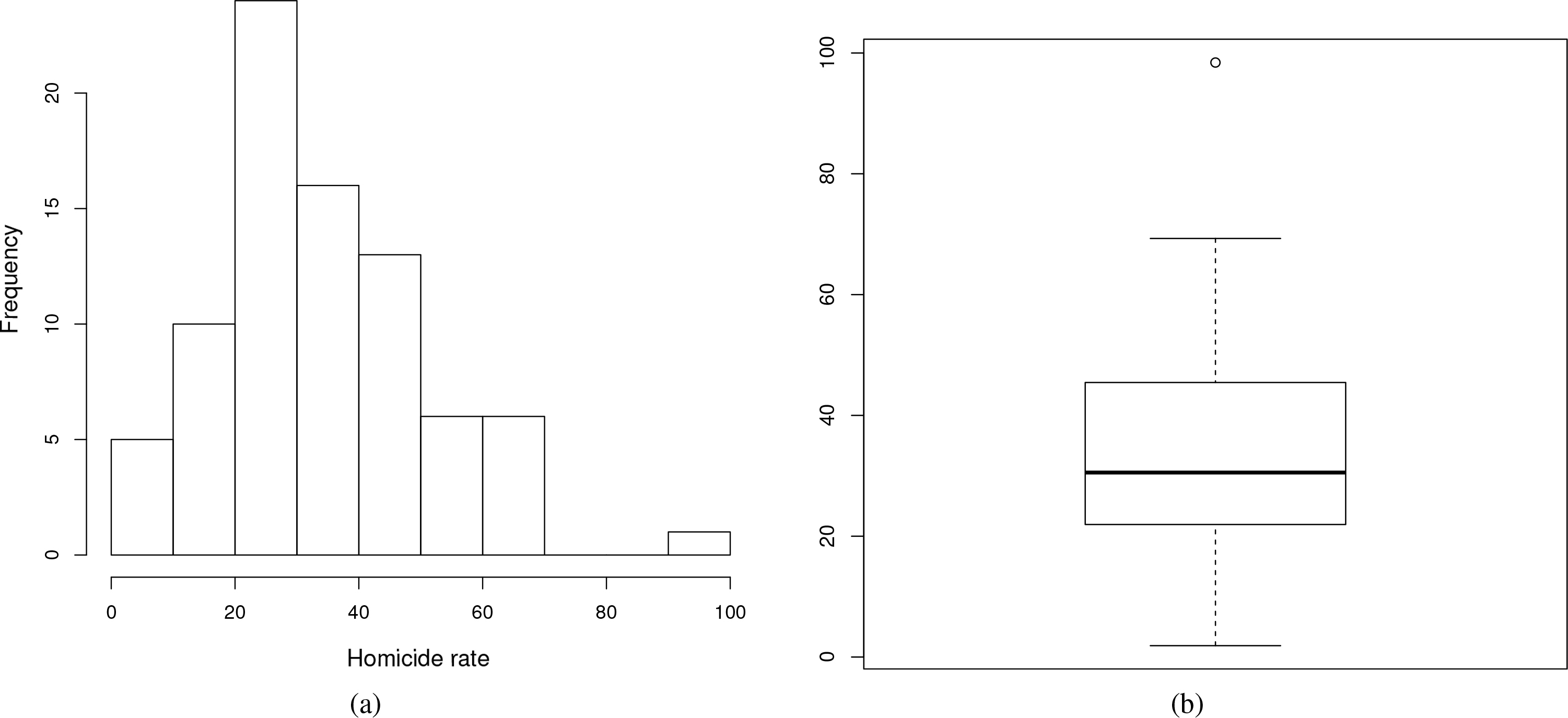

The systematic components for both beta and simplex regressions are defined by

$\displaystyle\text{logit}(\mu_{i})=\beta_{0}+\beta_{1}\text{time}_{i}+\beta_{2% }\text{GINI}_{i}+\beta_{3}\text{MHDI}_{i}+\beta_{4}\text{illiteracy}_{i}+\beta% _{5}\text{poverty}_{i}$

and

$\displaystyle h(\sigma_{i})=\gamma_{0}+\gamma_{1}\text{time}_{i}+\gamma_{2}% \text{GINI}_{i}+\gamma_{3}\text{MHDI}_{i}+\gamma_{4}\text{illiteracy}_{i}+% \gamma_{5}\text{poverty}_{i},$

where $\text{logit}(\mu_{i})=\log[\mu_{i}/(1-\mu_{i})]$ , and $h(\sigma_{i})=\text{logit}(\sigma_{i})$ for the beta regression and $h(\sigma_{i})=\log(\sigma_{1})$ for the simplex regression.

Table 2 lists the MLEs, their standard errors (SEs) and $p$ -values. In Table 3, we consider the following statistics: the global deviance (GD), Akaike Information Criterion (AIC) and Bayesian Information Criterion (BIC). The lower the values of these statistics, the better the fit. Based on these measures as selection criteria, the beta regression is more appropriate for these data.

Table 2
Results from the fitted complete beta and simplex regressions

Beta Simplex

$\bm{\beta}$ Estimate SE $p$ -value $\bm{\beta}$ Estimate SE $p$ -value

Intercept 2.232 2.308 0.337 Intercept 1.191 2.505 0.635

Time 0.949 0.207 $<$ 0.001 Time 0.196 0.001 $<$ 0.001

GINI 5.136 3.461 0.142 GINI 5.223 3.621 0.153

MHDI $-$ 9.337 2.759 0.001 MHDI $-$ 8.359 2.733 0.003

Illiteracy 0.013 0.036 0.712 Illiteracy 0.049 0.042 0.252

Poverty $-$ 0.045 0.019 0.020 Poverty $-$ 0.043 0.018 0.021

$\bm{\gamma}$ Estimate SE $p$ -value $\bm{\gamma}$ Estimate SE $p$ -value

Intercept $-$ 9.306 3.550 0.010 Intercept $-$ 10.858 3.187 0.001

Time $-$ 0.122 0.264 0.645 Time $-$ 0.485 0.221 0.032

GINI 15.359 5.033 0.003 GINI 15.330 4.396 0.001

MHDI $-$ 0.543 3.845 0.888 MHDI 3.677 3.271 0.264

Illiteracy 0.073 0.050 0.155 Illiteracy 0.123 0.038 0.002

Poverty $-$ 0.046 0.026 0.086 Poverty $-$ 0.038 0.024 0.115

Table 3
Goodness-of-fit measures for the homicide rate data

Model GD AIC BIC

Beta $-$ 85.340 $-$ 61.340 $-$ 32.600

Simplex $-$ 70.520 $-$ 46.520 $-$ 17.790

The numbers in Table 2 reveal that some explanatory variables are non-significant at the 5% level. Thus, the non-significant covariates were eliminated from the regressions based on the $p$ -values. Further, the fitted beta and simplex regressions considering only significant explanatory variables are reported in Table 4. The values in Table 5 indicate that the smaller GD, AIC and BIC statistics correspond to the reduced beta regression. So, we can conclude that this regression is the most suitable for modeling the current data.

Table 4
Results from the fitted reduced beta and simplex regressions

Beta Simplex

$\bm{\theta}$ Estimate SE $p$ -value $\bm{\beta}$ Estimate SE $p$ -value

Intercept 4.468 1.637 0.007 Intercept 4.515 1.845 0.016

Time 0.970 0.205 $<$ 0.001 Time 1.055 0.203 $<$ 0.001

MHDI $-$ 8.440 2.409 0.001 MHDI $-$ 8.612 2.631 $<$ 0.001

Poverty $-$ 0.028 0.013 0.043 Poverty $-$ 0.027 0.016 0.085

$\bm{\gamma}$ Estimate SE $p$ -value $\bm{\gamma}$ Estimate SE $p$ -value

Intercept $-$ 8.468 2.315 0.001 Intercept $-$ 6.144 1.837 0.001

GINI 12.902 3.958 0.001 GINI 11.255 3.225 0.008

Illiteracy 0.090 0.041 0.033 Illiteracy 0.097 0.034 0.005

Poverty $-$ 0.044 0.018 0.016 Poverty $-$ 0.037 0.014 0.008

Table 5
Goodness-of-fit measures considering only significant covariates

Regression model GD AIC BIC

Beta $-$ 82.120 $-$ 66.120 $-$ 46.970

Simplex $-$ 60.530 $-$ 44.530 $-$ 25.380

We now provide some conclusions about the fitted reduced beta regression which includes in the mean systematic component an intercept, time ( $\beta_{1}$ ), MHDI ( $\beta_{3}$ ) and poverty ( $\beta_{5}$ ). The positive sign of $\beta_{1}$ indicates that the mean homicide rate in the capital increases over time, assuming that both MHDI and poverty are fixed. As expected, increased quality of living conditions is associated with a lower incidence of homicides ( $\hat{\beta}_{3}=-8.440$ and $p$ -value $=0.001$ ). Unlike Blau and Blau (1982) and Messner (1982) who do not find statistically significant relationships between poverty and murder, the results indicate a small negative correlation between these variables ( $\hat{\beta}_{5}=-0.028$ and $p$ -value = $0.043$ ). Messner (1982) investigated the relationship between poverty, inequality and homicides for a sample of 204 metropolitan agglomerations and their results “suggest the need for reconsideration of the role of economic and perhaps subcultural factors in the explanation of urban homicide”. Like Messner (1982), the non-significant result of $\beta_{3}$ (GINI) indicates no association between income inequality and mean homicide rate. Pridemore (2011) argued that the effect of income concentration on homicides disappears by controlling for observed levels of poverty. Indeed, the inclusion of the poverty variable seems to have an independent effect on the mean murder rate. In particular, our estimate suggests that the higher the poverty rate, the lower the incidence of homicidal violence. In fact, we can interpret this by saying that the armed violence of gangsters is lower in very poor Brazilian capitals.

We calculate the case-deletion measures $\textit{GD}_{i}(\bm{\theta})$ and $\textit{LD}_{i}(\bm{\theta})$ defined in Section 2.3. The results of such influence measure index plots are presented in Fig. 2 for the beta regression. These plots reveal that two cases ( $\sharp$ 42 and $\sharp$ 79) for the beta regression are possible influential observations. The 42th city corresponds to Maceió (in 2010) which has the highest homicide rate. The 79th city refers to Vitória (in 1991) which has the second highest homicide rate. In this case, the beta regression can better model extreme observations than the simplex regression.

Figure 2.
Index plots for the reduced beta regression: (a) 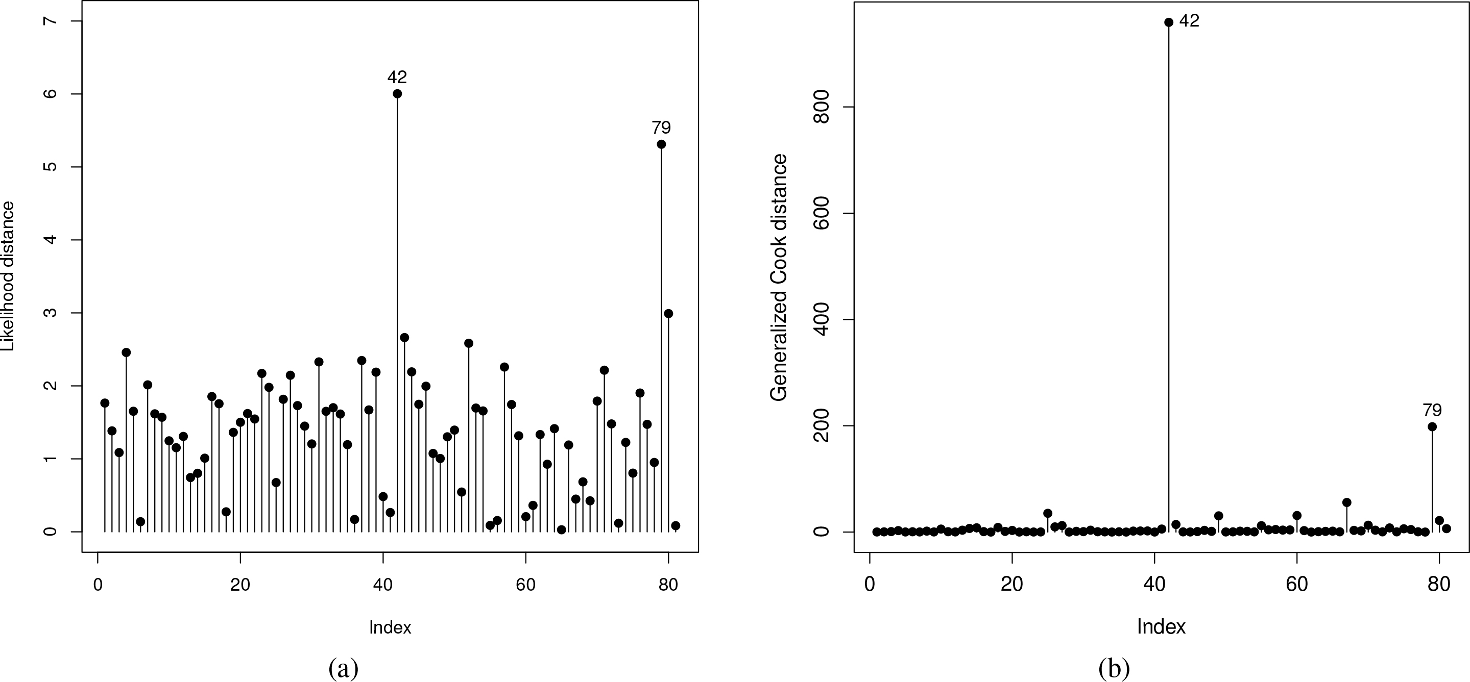$LD_{i}(\bm{\theta})$ (likelihood distance) and (b) $GD_{i}(\bm{\theta})$ (generalized Cook’s distance).

Figure 3.
Residual analysis for the reduced beta regression considering only significant covariates in 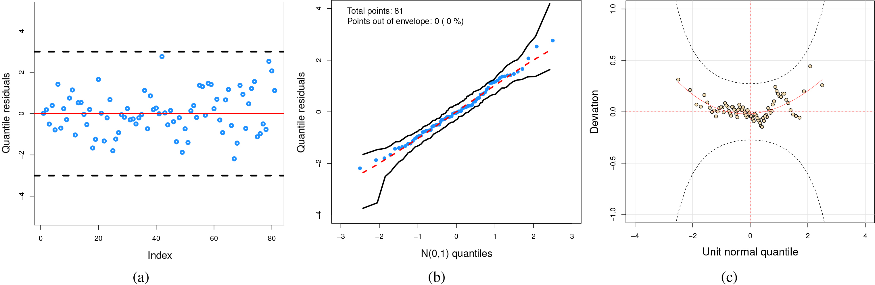$\mu$ and $\sigma$ . (a) Residuals versus index. (b) Simulated envelope. (a) Wormplot.

The plots of the quantile residuals versus the order of the observations for the fitted reduced beta regression is displayed in Fig. 3a. In these plot, we can note the random distribution of the residuals. As measure of fit quality, Fig. 3b display the normal probability plots and the simulated envelope for the fitted reduced beta regression, respectively. These plot indicate that there is no evidence of serious departures from the model assumptions of the fitted reduced beta regression. Thus, there is a clear evidence that the beta regression is better suited to the current data than the simplex regression. We display the wormplots for the fitted reduced beta regression in Fig. 3c. Based on these plot, we conclude that the beta regression with systematic components for $\mu$ and $\sigma$ is more suitable for modeling the homicide rates.
4.1 Findings for the mean homicide rates

Beta	Simplex
Intercept	2.232	2.308	0.337	Intercept	1.191	2.505	0.635
Time	0.949	0.207	$<$ 0.001	Time	0.196	0.001	$<$ 0.001
GINI	5.136	3.461	0.142	GINI	5.223	3.621	0.153
MHDI	$-$ 9.337	2.759	0.001	MHDI	$-$ 8.359	2.733	0.003
Illiteracy	0.013	0.036	0.712	Illiteracy	0.049	0.042	0.252
Poverty	$-$ 0.045	0.019	0.020	Poverty	$-$ 0.043	0.018	0.021
$\bm{\gamma}$	Estimate	SE	$p$ -value	$\bm{\gamma}$	Estimate	SE	$p$ -value
Intercept	$-$ 9.306	3.550	0.010	Intercept	$-$ 10.858	3.187	0.001
Time	$-$ 0.122	0.264	0.645	Time	$-$ 0.485	0.221	0.032
GINI	15.359	5.033	0.003	GINI	15.330	4.396	0.001
MHDI	$-$ 0.543	3.845	0.888	MHDI	3.677	3.271	0.264
Illiteracy	0.073	0.050	0.155	Illiteracy	0.123	0.038	0.002
Poverty	$-$ 0.046	0.026	0.086	Poverty	$-$ 0.038	0.024	0.115

Model	GD	AIC	BIC
Beta	$-$ 85.340	$-$ 61.340	$-$ 32.600
Simplex	$-$ 70.520	$-$ 46.520	$-$ 17.790

Beta	Simplex
Intercept	4.468	1.637	0.007	Intercept	4.515	1.845	0.016
Time	0.970	0.205	$<$ 0.001	Time	1.055	0.203	$<$ 0.001
MHDI	$-$ 8.440	2.409	0.001	MHDI	$-$ 8.612	2.631	$<$ 0.001
Poverty	$-$ 0.028	0.013	0.043	Poverty	$-$ 0.027	0.016	0.085
$\bm{\gamma}$	Estimate	SE	$p$ -value	$\bm{\gamma}$	Estimate	SE	$p$ -value
Intercept	$-$ 8.468	2.315	0.001	Intercept	$-$ 6.144	1.837	0.001
GINI	12.902	3.958	0.001	GINI	11.255	3.225	0.008
Illiteracy	0.090	0.041	0.033	Illiteracy	0.097	0.034	0.005
Poverty	$-$ 0.044	0.018	0.016	Poverty	$-$ 0.037	0.014	0.008

Regression model	GD	AIC	BIC
Beta	$-$ 82.120	$-$ 66.120	$-$ 46.970
Simplex	$-$ 60.530	$-$ 44.530	$-$ 25.380

More findings can follow from the beta regression estimates in Table 4.

•
The time is significant, i.e., the mean homicide rate tends to increase as the time goes by. These results are consistent with the aggregate analysis by federation unit which indicates a positive trend of homicidal violence in Brazil (1996–2017). Despite recent reductions (2018 and 2019), official data have not yet been released, making it difficult to assess the consistency of negative fluctuation over the past two years; see https://oglobo.globo.com/brasil/o-que-esta-por-tras-da-qual-eda-de-pais-em-2019-23900239. Perhaps it is the case to report the rate of the national homicide series (Brazil, 1996–2017).
•
The MHDI is also a significant covariate and the average homicide rate tends to increase when this index decreases. In fact, the negative sign of the estimate $\hat{\beta}_{3}$ reveals that the increase in quality of life is associated with a reduction in homicides. It is more intuitive to interpret the variation of the independent variable in a positive sense. This finding is consistent with part of the literature on the subject that explores the correlation between socioeconomic variables and levels of violence. For example, Fajnzylber et al. (2002) examined the relationship between income inequality, homicides and violent crimes from a longitudinal database. The authors found a correlation between these variables and considered a causal function between income inequality and violent crimes. Messner et al. (2002) also found statistically significant associations between homicides and income inequality.
•
The poverty is significant and the mean homicide rate tends to decrease slightly when poverty proportion increases. This finding is curious given the lower correlation between MHDI and poverty. Another interesting issue is the independent effect of the poverty, even controlled by the MHDI. The higher the poverty, the lower the mean homicide rate. These results corroborate Messner’s (1982) proposition about the need to review the causal link between poverty and violence.

In the beta regression model, we emphasize that the homicide rate variability increases when the dispersion parameter $\sigma$ increases.
4.2 Findings for the dispersion homicide rates

•
As the time passes, the estimated dispersion parameter of the homicide rate decreases, assuming the other variables fixed.
•
The GINI coefficient is significant in relation to the dispersion homicide rate, i.e., this dispersion is expected to increase when the GINI increases. This finding is consistent with the literature that examines the relationship between income inequality and homicidal violence (Kelly, 2000; Neumayer, 2005). These results have direct implications for the formulation and implementation of public policies specially designed to reduce income asymmetry.
•
The illiteracy rate is significant in relation to the dispersion parameter. The positive sign of $\hat{\gamma}_{4}$ reveals that the homicide rate dispersion tends to increase when higher illiteracy proportions. We believe that this paper presents the first systematic evidence relating the illiteracy rate to the homicide rate dispersion. In particular, this result indicates that the more heterogeneous the distribution of illiteracy, the greater the dispersion of the homicide rate.
•
Finally, the poverty proportion is also significant in relation to the dispersion homicide rate. This dispersion tends to decrease for capitals with greater variability of wealth.

5. Concluding remarks

The primary purpose of this paper is to quantify some explanatory variables that influence homicide rates in Brazil using the most important regression models for proportional data. We construct beta and simplex regressions with two systematic components for the mean and dispersion parameters for modeling the homicide rates in the Brazilian capitals. The response variable refers to the homicide rates measured by the number of homicides in the city normalized by its total population with data from the 1990s and 2000s. We consider as explanatory variables: the time, the GINI coefficient as measure of income inequality, municipal human development index (MHDI), illiteracy and poverty rates. We adopt standard methods based on likelihood theory to estimate the model parameters and select the best regression. We evaluate important findings to look for the effects of the explanatory variables on the mean and dispersion homicide rates. The analysis shows that the beta regression provides better estimates for these data and provide some more substantive conclusions about the explanatory variables that influence homicide rates in Brazil. Our results can be useful for future research on homicides prevention and enhance our understanding of which factors influence murder rate in extreme violent countries.

Footnotes

Acknowledgments

We are very grateful to a referee and Co-Editor-in-Chief for helpful comments that considerably improved the paper. We gratefully acknowledge financial support from CAPES and CNPq.

References

Atkinson

A. C.

(1985). Plots, transformations, and regression: An introduction to graphical methods of diagnostic regression analysis. Oxford: Clarendon Press Oxford.

Barndorff-Nielsen

O. E.

, & Jrgensen

(1991). Some parametric models on the simplex. Journal of Multivariate Analysis, 39, 106-116.

Blau

J. R.

, & Blau

P. M.

(1982). The cost of inequality: Metropolitan structure and violent crime. American Sociological Review, 47, 114-129.

Braithwaite

, & Braithwaite

(1980). The effect of income inequality and social democracy on homicide: A cross-national comparison. The British Journal of Criminology, 20, 45-53.

Buuren

S. V.

, & Fredriks

(2001). Worm plot: A simple diagnostic device for modelling growth reference curves. Statistics in Medicine, 20, 1259-1277.

Dunn

P. K.

, & Smyth

G. K.

(1996). Randomized quantile residuals. Journal of Computational and Graphical Statistics, 5, 236-244.

Eisner

(2003). Long-term historical trends in violent crime. Crime and Justice, 30, 83-142.

Fajnzylber

Lederman

, & Loayza

(2002). Inequality and violent crime. The Journal of Law and Economics, 45, 1-39.

Ferrari

and Cribari- Neto

(2004). Beta regression for modelling rates and proportions. Journal of Applied Statistics, 31, 799-815.

10.

Gartner

(1990). The victims of homicide: A temporal and cross-national comparison. American Sociological Review, 55, 92-106.

11.

Kelly

(2000). Inequality and crime. Review of Economics and Statistics, 82, 530-539.

12.

Krohn

M. D.

(1976). Inequality, unemployment and crime: A cross-national analysis. The Sociological Quarterly, 17, 303-313.

13.

Loftin

, & Hill

R. H.

(1974). Regional subculture and homicide: An examination of the Gastil-Hackney thesis. American Sociological Review, 39, 714-724.

14.

Mc Donald

(1976). The Sociology of Law and Order. London, Faber and Faber.

15.

Messner

S. F.

(1982). Poverty, inequality, and the urban homicide rate: Some unexpected findings. Criminology, 20, 103-114.

16.

Messner

S. F.

Raffalovich

L. E.

, & Shrock

(2002). Reassessing the cross-national relationship between income inequality and homicide rates: Implications of data quality control in the measurement of income distribution. Journal of Quantitative Criminology, 18, 377-395.

17.

Neumayer

(2005). Inequality and violent crime: Evidence from data on robbery and violent theft. Journal of Peace Research, 42, 101-112.

18.

Nivette

A. E.

(2011). Cross-national predictors of crime: A meta-analysis. Homicide Studies, 15, 103-131.

19.

Parker

R. N.

, & Smith

M. D.

(1979). Deterrence, poverty, and type of homicide. American Journal of Sociology, 85, 614-624.

20.

Parker

R. N.

, & Loftin

(1983). Poverty, inequality, and type of homicide: A reconsideration of unexpected results. In Annual Meeting of the American Society of Criminology, Denver, Nov 83.

21.

Pridemore

W. A.

(2011). Poverty matters: A reassessment of the inequality homicide relationship in cross-national studies. The British Journal of Criminology, 51, 739-772.

22.

Rigby

R. A.

, & Stasinopoulos

D. M.

(2005). Generalized additive models for location, scale and shape (with discussion). Appl Statist, 54, 507-554.

23.

Roberts

, & Willits

(2015). Income inequality and homicide in the United States: Consistency across different income inequality measures and disaggregated homicide types. Homicide Studies, 19, 28-57.

24.

Rocha

A. V.

, & Simas

A. B.

(2011). Influence diagnostics in a general class of beta regression models. Test, 20, 95-119.

25.

Song

PX-K

, & Tan

(2000). Marginal models for longitudinal continuous proportional data. Biometrics, 56, 496-502.

26.

Stasinopoulos

D. M.

, & Rigby