Random order autoregressive time series model with structural break

Abstract

This paper deals with the problem of modelling time series data with structural breaks occur at multiple time points that may result in varying order of the model at every structural break. A flexible and generalized class of Autoregressive (AR) models with multiple structural breaks is proposed for modelling in such situations. Estimation of model parameters are discussed in both classical and Bayesian frameworks. Since the joint posterior of the parameters is not analytically tractable, we employ a Markov Chain Monte Carlo method, Gibbs sampling to simulate posterior sample. To verify the order change, a hypotheses test is constructed using posterior probability and compared with that of without breaks. The methodologies proposed here are illustrated by means of simulation study and a real data analysis.

Keywords

Autoregressive model Bayesian estimation Gibbs sample order changed model structural break

1. Introduction

In the fast-growing world, data observed on chronological order show dynamical phenomenon of significant growth occurred due to implementation of new government policy, new technology and other policies. Such phenomena may often exhibit structural changes over a period of time. At a structural break, changes may occur in process mean, error variation and trends. An extensive study took place in this field. Perron (1990), Perron and Vogelsang (1992), Zivot and Andrews (1992), Chib (1998), Lee and Strazicich (2003), Maddala and Kim (2003), Chaturvedi and Kumar (2007), Shao and Zhang (2010) among others addressed the problem of testing, detection and estimation under structural breaks in the mean or trend. They demonstrated various applications in oil price, stock market and GNP growth rate etc using classical and Bayesian methods of estimation. The problem of modelling of structural breaks with varying error variance has been addressed by Inclan (1993), Kim et al. (2002), Cook (2002), Kumar et al. (2012) and Kim et al. (2002). In the literature cite above, the problem of structural breaks in mean and error variance are addressed for both univariate and multivariate setups (see Bai, 2010; Meligkotsidou et al., 2011 and Eo, 2016). Meligkotsidou et al. (2017) and Slama and Saggou (2017) also conceded the multiple break points in autoregressive coefficient and applied Bayesian significance test to detect the change occurs in the parameters. Most of the authors considered AR(1) model for detecting structural breaks in association with unit root, see Perron (1990), Perron and Vogelsang (1992), Zivot and Andrews (1992), Inclan (1993), Chib (1998). However, the following literature, Wang and Zivot (2000), Meligkotsidou et al. (2017), Vosseler (2016), Slama and Saggou (2017) considered the problem of estimation and testing under single or multiple breaks for general AR(p) model.

In the above studies, the order of AR model is assumed to be predetermined at each structural break and only changes in model parameters are considered. That seems to be unrealistic for real life situations since characteristics of any random phenomenon do not remain constant and priory know due to inherent uncertainty. A process may also change from one order (lag) to another order (lag) due to presence of structural break, known as order change process. For example, in economic and finance series a great depression was occurred in oil price stocks due to sudden changes in economic policy and stock market trading which shifted the structure of series. Therefore, this article aims to propose a flexible and generalized AR(p) model where the order of the model is assumed to be unknown and to be estimated from the given time series data. Thus, proposed method will have potential to model the situation where the AR process completely changes it’s order at each break point.

The problem of Bayesian estimation for autoregressive process under structural break is discussed by many authors. Broemeling (1972) discussed the change point problem with known variance and construct Bayesian estimators of the parameters under non-informative priors. Smith (1975) discussed the problem of change point based on the posterior probability of the possible change. A Bayesian significance test for stationarity of a regression model was proposed by Kim (1991). Barbieri and Conigliani (1998) derived a Bayes factor for identification of a change in mean of a stationary autoregressive model. Kezim and Abdelli (2004) studied a Bayesian analysis of an AR(1) model subject to one change in both error variance and autocorrelation coefficient. Meligkotsidou et al. (2011) considered structural change in level, error variance and autoregressive coefficient at unknown break point and estimation the model parameters by using marginal likelihood. Kumar et al. (2012) investigated the impact of structural break in error variance using Bayesian framework and applied on export data of selected ASEAN countries for AR(1) time series model.

The objective of the paper is many folds. First objective is to introduce an order change autoregressive model (O-AR) in consideration for structural breaks on other parameters of the series. Second is to develop maximum likelihood and Bayesian estimation methods for estimating the unknown parameters of the model. Finally, we examine the impact of such change on its regression parameters as well as order. Rest of the manuscript is organized in the following sections. The proposed model is stated in Section 2. Considering change in mean, variance and trend, four different models are given with order change. The maximum likelihood estimation is used to estimate the parameters. Bayesian estimation is discussed in Section 3. Considering conjugate prior distributions, Bayes estimation is performed under two symmetric loss functions, squared error loss and absolute loss. Posterior probability is used for detecting an arbitrary change in the order as well as breaks in mean and error variance of an autoregressive time series model under the assumption that order of the model at each break is known. To evaluate the performance of our proposed model, a simulation study and an empirical analysis of natural gas series of United State are carried out in Sections 4 and 5 respectively. At the end of the paper, conclusions are stated in Section 6.

2. Model specification

In this section, we consider a univariate autoregressive time series model of order p which is generated through the stochastic process $\{y_{t},t\in Z\}$ , where $Z$ is a set of positive integers. The AR(p) model is given by

$\displaystyle y_{t}=\theta+\phi_{1}y_{t-1}+\phi_{2}y_{t-2}+\ldots+\phi_{p}y_{t% -p}+\varepsilon_{t},\quad t=1,2,\ldots,T,$ (1)

where $\theta$ and $\phi=\{{\phi_{1},\phi_{2},\ldots,\phi_{P}}\}$ be the intercept and autoregressive coefficients, respectively. Error $\varepsilon_{t}$ is a sequence of i.i.d. normal random variable with mean zero and variance $\sigma^{2}$ .

Mainly, structural breaks take place when parameters of the model are shifted or changed permanently from one period to another period for a given series. In many cases, breaks do not affect only parameters but also affect the order p of autoregressive time series model. If the change in order of AR process is not taken place with the change on autoregressive coefficients, then this may be termed as misidentifications. So, it is equally important to consider the structural break with order change too. The main motivation of present study is to explore AR model which allows break on all parameters with the change on order. One may also be interested to explore the model where some parameters may not have exposed by the structural break. Therefore, we are formulating following models in respect to the various break(s) situations:

M1: Autoregressive model with change on order but no change on mean and variance. M2: Autoregressive model with change on order and mean but no change in variance. M3: Autoregressive model with change on order and error variance but no change on mean. M4: Autoregressive model with change on order, mean and error variance.

Let $N_{T}$ be the total number of structural break points at which model it bears the changes on parameters, $n_{i}=k_{i+1}-k_{i}$ observations present in the $i^{\text{th}}$ regime with order $p_{i}$ where $i=0,1,2,\ldots,N_{t}$ . Without loss of generality, we may use $k_{0}=0$ and $k_{N_{t}+1}=T$ . The AR model in Eq. (1) under model condition M1.

$\displaystyle y_{t}^{(i)}=\theta+\phi_{1}^{(i)}y_{t-1}^{(i)}+\phi_{2}^{(i)}y_{% t-2}^{(i)}+\ldots+\phi_{p_{i}}^{(i)}y_{t-p_{i}}^{(i)}+\varepsilon_{t},\quad k_% {i}<t\leqslant k_{i+1}.$ (2)

For mathematical manipulation, we may write model in Eq. (2) in matrix form,

$\displaystyle Y_{i}=\theta l_{n_{i}}+X_{i}\beta_{i}+E_{i},\quad i=0,1,2,\ldots% ,N_{T},$ (3)

where $l_{n_{i}}$ be a $n_{i}\times$ 1 vector with all elements one, $Y_{i}=({y_{k_{i}+1}^{(i)}}∼{}∼{}{y_{k_{i}+2}^{(i)}}∼{}∼{}\ldots∼{}∼{}{y_{k_{i+% 1}}^{(i)}})^{\prime},\\ X_{i}=\begin{pmatrix}{y_{k_{i}}^{(i)}}&{y_{k_{i}-1}^{(i)}}&\ldots&{y_{k_{i}+1-% p_{i}}^{(i)}}\\ {y_{k_{i}+1}^{(i)}}&{y_{k_{i}}^{(i)}}&\ldots&{y_{k_{i}+2-p_{i}}^{(i)}}\\ \vdots&\vdots&\ddots&\vdots\\ {y_{k_{i+1}-1}^{(i)}}&{y_{k_{i+1}-2}^{(i)}}&\ldots&{y_{k_{i+1}-p_{i}}^{(i)}}% \end{pmatrix},\beta_{i}=({\phi_{1}^{(i)}}∼{}∼{}{\phi_{2}^{(i)}}∼{}∼{}\ldots∼{}% ∼{}{\phi_{p_{i}}^{(i)}})^{\prime},E_{i}=({e_{k_{i}+1}^{(i)}}∼{}∼{}{e_{k_{i}+2}% ^{(i)}}∼{}∼{}\ldots∼{}∼{}{e_{k_{i+1}}^{(i)}})^{\prime}$ .

Similarly, model Eq. (1) may be written as under model condition M2

$\displaystyle Y_{i}=\theta_{i}l_{n_{i}}+X_{i}\beta_{i}+E_{i},\quad i=0,1,2,% \ldots,N_{T},$ (4)

and under model condition M3, model Eq. (1) expressed as

$\displaystyle Y_{i}=\theta l_{n_{i}}+X_{i}\beta_{i}+\sigma_{i}E_{i},\quad i=0,% 1,2,\ldots,N_{T},$ (5)

Above model Eq. (3) to Eq. (5), allow break on parameters one by one. However, our main interest is to study the model which allows break on all parameters. Under model condition M4, we get the model

$\displaystyle Y_{i}=\theta_{i}l_{n_{i}}+X_{i}\beta_{i}+\sigma_{i}E_{i},\quad i% =0,1,2,\ldots,N_{T}.$ (6)

Here it is noted that Model M1–M3 are the particular case of Model M4. In classical approach, the most commonly used estimation method is maximum likelihood method which is obtained by maximizing the likelihood or equivalently log-likelihood function. The likelihood functions for models M1–M4 are respectively obtained by

$\displaystyle L({\Theta_{1}|Y})=\left({\frac{1}{2\pi}}\right)^{\frac{T}{2}}% \left({\frac{1}{\sigma^{2}}}\right)^{\frac{T}{2}}\prod\limits_{i=0}^{N_{T}}{% \exp\left[{-\frac{1}{2\sigma^{2}}({Y_{i}-\theta l_{n_{i}}-X_{i}\beta_{i}})^{% \prime}({Y_{i}-\theta l_{n_{i}}-X_{i}\beta_{i}})}\right]},$ (7) $\displaystyle L({\Theta_{2}|Y})=\left({\frac{1}{2\pi}}\right)^{\frac{T}{2}}% \left({\frac{1}{\sigma^{2}}}\right)^{\frac{T}{2}}\prod\limits_{i=0}^{N_{T}}{% \exp\left[{-\frac{1}{2\sigma^{2}}({Y_{i}-\theta_{i}l_{n_{i}}-X_{i}\beta_{i}})^% {\prime}({Y_{i}-\theta_{i}l_{n_{i}}-X_{i}\beta_{i}})}\right]},$ (8) $\displaystyle L({\Theta_{3}|Y})=\left({\frac{1}{2\pi}}\right)^{\frac{T}{2}}% \prod\limits_{i=0}^{N_{T}}{\left({\frac{1}{\sigma_{i}^{2}}}\right)^{\frac{n_{i% }}{2}}\exp\left[{-\frac{1}{2\sigma_{i}^{2}}({Y_{i}-\theta l_{n_{i}}-X_{i}\beta% _{i}})^{\prime}({Y_{i}-\theta l_{n_{i}}-X_{i}\beta_{i}})}\right]},$ (9) $\displaystyle L({\Theta_{4}|Y})=\left({\frac{1}{2\pi}}\right)^{\frac{T}{2}}% \prod\limits_{i=0}^{N_{T}}{\left({\frac{1}{\sigma_{i}^{2}}}\right)^{\frac{n_{i% }}{2}}\exp\left[{-\frac{1}{2\sigma_{i}^{2}}({Y_{i}-\theta_{i}l_{n_{i}}-X_{i}% \beta_{i}})^{\prime}({Y_{i}-\theta_{i}l_{n_{i}}-X_{i}\beta_{i}})}\right]},$ (10)

where,

$\displaystyle\Theta_{1i}=\{{\theta,\beta_{i},\sigma^{2}}\},\Theta_{1}=\{{% \Theta_{10},\Theta_{11},\ldots,\Theta_{1N_{T}}}\}\Theta_{2i}=\{{\theta_{i},% \beta_{i},\sigma^{2}}\},\Theta_{2}=\{{\Theta_{20},\Theta_{21},\ldots,\Theta_{2% N_{T}}}\},$ $\displaystyle\Theta_{3i}=\{{\theta,\beta_{i},\sigma_{i}^{2}}\},\Theta_{3}=\{{% \Theta_{30},\Theta_{31},\ldots,\Theta_{3N_{T}}}\}\Theta_{4i}=\{{\theta_{i},% \beta_{i},\sigma_{i}^{2}}\},\Theta_{4}=\{{\Theta_{40},\Theta_{41},\ldots,% \Theta_{4N_{T}}}\}.$

The general forms of the maximum likelihood estimators of the parameters can be obtained as,

$\displaystyle\hat{\Theta}=(Z^{\prime}Z)^{-1}Z^{\prime}Y,∼{}\hat{\sigma}^{2}=% \frac{(Y-\hat{Y})^{\prime}(Y-\hat{Y})}{s-r},$ (11)

where, $r$ is the number of parameters and $Z=({l_{n_{i}},X_{i}})$ .

All model conditions M1–M4 allows break in respective parameters and one may be interested to test that there is a break or not. That can be stated with the following hypothesis. Under model M1: $H_{0}:p_{i}=p_{j}$ versus $H_{1}:p_{i}\neq p_{j}$ , with, $\theta_{i}=\theta_{j},\sigma_{i}^{2}=\sigma_{j}^{2}$ . Under model M2: $H_{0}:p_{i}=p_{j},\theta_{i}=\theta_{j}$ versus $H_{1}:p_{i}\neq p_{j},\theta_{i}\neq\theta_{j}$ , with, $\sigma_{i}^{2}=\sigma_{j}^{2}$ . Under model M3: $H_{0}:p_{i}=p_{j},\sigma_{i}^{2}=\sigma_{j}^{2}$ versus $H_{1}:p_{i}\neq p_{j},\sigma_{i}^{2}\neq\sigma_{j}^{2},$ with, $\theta_{i}=\theta_{j}.$ Under model M4: $H_{0}:p_{i}=p_{j},\theta_{i}=\theta_{j},\sigma_{i}^{2}=\sigma_{j}^{2}$ versus $H_{1}:p_{i}\neq p_{j},\theta_{i}\neq\theta_{j},\sigma_{i}^{2}\neq\sigma_{j}^{2}$ . Although, these hypotheses can be tested using various approach, we explored this under Bayesian framework using posterior probability.

3. Bayesian inference

Bayesian inference allows to use the information available with data by likelihood function and information about the parameters by prior information together which produces the joint posterior distribution as defined by,

$\displaystyle P({\Theta|Y})\propto L({\Theta|Y})P(\Theta)$

The joint posterior distribution of $\Theta$ is constricted using the following prior distributions,

(iii) (i)
The $N_{T}+1$ values of $\sigma_{i}^{2}$ are conditionally independent draw from the inverse gamma distribution with parameter “ $a$ ” and “ $b$ ”.
(ii)
$\beta_{i}\sim MN(\mu_{i},\sigma_{i}^{2}I_{p_{i}})$
(iii)
$\theta_{i}\sim N(\delta_{i},\sigma_{i}^{2})$
(iv)
For change point parameter, all possible location of break $k_{1}<k_{2}<k_{3}<\ldots<k_{N_{T}}$ are assume to equal probability that is $P(k|N_{T})=\begin{pmatrix}T-1\\ N_{T}\end{pmatrix}^{-1}$

The joint posterior distribution for models M1 to M4 are respectively given by

$\displaystyle P({\Theta_{1}|M1})=\left({\frac{1}{2\pi}}\right)^{\frac{T+1}{2}}% \left({\frac{b^{\rm a}}{\Gamma a}}\right)\left({\frac{1}{\sigma^{2}}}\right)^{% \frac{T+1}{2}+a+1}\begin{pmatrix}{T-1}\\ {N_{T}}\end{pmatrix}^{-1}\prod\limits_{i=0}^{N_{T}}{\left({\frac{1}{2\pi}}% \right)^{\frac{p_{i}}{2}}\left({\frac{1}{\sigma^{2}}}\right)^{\frac{p_{i}}{2}}}$ $\displaystyle\exp\left[{-\frac{1}{2\sigma^{2}}\left\{{\sum_{i=0}^{N_{T}}{({({Y% _{i}-\theta l_{n_{i}}-X_{i}\beta_{i}})^{\prime}({Y_{i}-\theta l_{n_{i}}-X_{i}% \beta_{i}})+({\beta_{i}-\mu_{i}})^{\prime}I_{p_{i}}^{-1}({\beta_{i}-\mu_{i}})}% )}+({\theta-\delta})^{2}+2b}\right\}}\right]$ $\displaystyle P({\Theta_{2}|M2})=\left({\frac{1}{2\pi}}\right)^{\frac{T}{2}}% \left({\frac{b^{\rm a}}{\Gamma a}}\right)\left({\frac{1}{\sigma^{2}}}\right)^{% \frac{T}{2}+a+1}\begin{pmatrix}{T-1}\\ {N_{T}}\end{pmatrix}^{-1}\exp\left[{-\frac{b}{\sigma^{2}}}\right]\prod\limits_% {i=0}^{N_{T}}{\left({\frac{1}{2\pi}}\right)^{\frac{p_{i}+1}{2}}\left({\frac{1}% {\sigma^{2}}}\right)^{\frac{p_{i}+1}{2}}}$ $\displaystyle\exp\left[{-\frac{1}{2\sigma^{2}}\sum_{i=0}^{N_{T}}{\{{({Y_{i}-% \theta_{i}l_{n_{i}}-X_{i}\beta_{i}})^{\prime}({Y_{i}-\theta_{i}l_{n_{i}}-X_{i}% \beta_{i}})+({\beta_{i}-\mu_{i}})^{\prime}I_{p_{i}}^{-1}({\beta_{i}-\mu_{i}})+% ({\theta_{i}-\delta_{i}})^{2}}\}}}\right]$ $\displaystyle P({\Theta_{3}|M3})=\left({\frac{1}{2\pi}}\right)^{\frac{T+1}{2}}% \left({\frac{b^{\rm a}}{\Gamma a}}\right)^{N_{T}+1}\left({\frac{1}{\tau}}% \right)^{\frac{1}{2}}\begin{pmatrix}{T-1}\\ {N_{T}}\end{pmatrix}^{-1}\exp\left[{-\frac{({\theta-\delta})^{2}}{2\tau}}% \right]\prod\limits_{i=0}^{N_{T}}{\left({\frac{1}{2\pi}}\right)^{\frac{p_{i}}{% 2}}}\left({\frac{1}{\sigma_{i}^{2}}}\right)^{\frac{p_{i}+n_{i}}{2}+a+1}$ $\displaystyle\exp\left[{-\sum_{i=0}^{N_{T}}{\frac{1}{2\sigma_{i}^{2}}\{{({Y_{i% }-\theta l_{n_{i}}-X_{i}\beta_{i}})^{\prime}({Y_{i}-\theta l_{n_{i}}-X_{i}% \beta_{i}})+({\beta_{i}-\mu_{i}})^{\prime}I_{p_{i}}^{-1}({\beta_{i}-\mu_{i}})+% 2b}\}}}\right]$ $\displaystyle P(\Theta_{4}|M4)=\left({\frac{1}{2\pi}}\right)^{\frac{T}{2}}% \left({\frac{b^{\rm a}}{\Gamma a}}\right)^{N_{T}+1}\begin{pmatrix}{T-1}\\ {N_{T}}\end{pmatrix}^{-1}\prod\limits_{i=0}^{N_{T}}{\left({\frac{1}{2\pi}}% \right)^{\frac{p_{i}+n_{i}}{2}}\left({\frac{1}{\sigma_{i}^{2}}}\right)^{\frac{% p_{i}+n_{i}}{2}+a+1}}$ $\displaystyle\exp\left[{-\sum_{i=0}^{N_{T}}{\frac{1}{2\sigma_{i}^{2}}}}\{{(Y_{% i}-\theta_{i}l_{n_{i}}-X_{i}\beta_{i})^{\prime}}{(Y_{i}-\theta_{i}l_{n_{i}}-X_% {i}\beta_{i})+(\beta_{i}-\mu_{i})^{\prime}I_{p_{i}}^{-1}(\beta_{i}-\mu_{i})+(% \theta_{i}-\delta_{i})^{2}+2b}\}\right]$

For hypothesis testing under Bayesian framework, we first obtain marginal posterior probability for each model and compare with other models. Marginal probability is obtained by integrated over the specified range of parameters. The marginal posterior probabilities for M1 to M4 are given by

$\displaystyle P({Y|M1})=\left({\frac{b^{\rm a}}{\Gamma a}}\right)(2\pi)^{{}^{-% \frac{T}{2}}}\begin{pmatrix}{T-1}\\ {N_{T}}\end{pmatrix}^{-1}\prod\limits_{i=0}^{N_{T}}{|{X_{i}^{\prime}X+I_{p_{i}% }^{-1}}|^{-\frac{1}{2}}}\frac{\Gamma\left({\frac{T}{2}+a}\right)}{({S_{1}})^{% \frac{T}{2}+a}}\prod\limits_{i=0}^{N_{T}}{|{l_{n_{i}}^{\prime}l_{n_{i}}-l_{n_{% i}}^{\prime}X_{i}(X_{i}^{\prime}X_{i}+I_{p_{i}}^{-1})^{-1}X_{i}^{\prime}l_{n_{% i}}}|^{-\frac{1}{2}}}$ $\displaystyle P({Y|M2})=\left({\frac{b^{\rm a}}{\Gamma a}}\right)(2\pi)^{{}^{-% \frac{T}{2}}}\begin{pmatrix}{T-1}\\ {N_{T}}\end{pmatrix}^{-1}\prod\limits_{i=0}^{N_{T}}{|{X_{i}^{\prime}X+I_{p_{i}% }^{-1}}|^{-\frac{1}{2}}}\frac{\Gamma\left({\frac{T}{2}+a}\right)}{({S_{2}})^{% \frac{T}{2}+a}}\prod\limits_{i=0}^{N_{T}}{|{l_{n_{i}}^{\prime}l_{n_{i}}+1-l_{n% _{i}}^{\prime}X_{i}(X_{i}^{\prime}X_{i}+I_{p_{i}}^{-1})^{-1}X_{i}^{\prime}l_{n% _{i}}}|^{-\frac{1}{2}}}$ $\displaystyle P({Y|M3})=\left({\frac{1}{2\pi}}\right)^{\frac{T+1}{2}}\left({% \frac{b^{\rm a}}{\Gamma a}}\right)^{N_{T}+1}\begin{pmatrix}{T-1}\\ {N_{T}}\end{pmatrix}^{-1}\prod\limits_{i=0}^{N_{T}}{|{X_{i}^{\prime}X+I_{p_{i}% }^{-1}}|^{-\frac{1}{2}}}\int_{-\infty}^{\infty}{\left({\frac{1}{\tau}}\right)^% {\frac{1}{2}}\prod\limits_{i=0}^{N_{T}}{\frac{\Gamma\left({\frac{n_{i}}{2}+a}% \right)}{({S_{3i}})^{\frac{n_{i}}{2}+a}}}\exp\left[{-\frac{1}{2\tau}({\theta-% \delta})^{2}}\right]}{\rm d}\theta$ $\displaystyle P({Y|M4})=\left({\frac{1}{2\pi}}\right)^{\frac{T}{2}}\left({% \frac{b^{\rm a}}{\Gamma a}}\right)^{N_{T}+1}\begin{pmatrix}{T-1}\\ {N_{T}}\end{pmatrix}^{-1}\prod\limits_{i=0}^{N_{T}}{|{X_{i}^{\prime}X+I_{p_{i}% }^{-1}}|^{-\frac{1}{2}}}\frac{\Gamma\left({\frac{n_{i}}{2}+a}\right)}{({S_{4i}% })^{\frac{n_{i}}{2}+a}}|{l_{n_{i}}^{\prime}l_{n_{i}}+1-l_{n_{i}}^{\prime}X_{i}% (X_{i}^{\prime}X_{i}+I_{p_{i}}^{-1})^{-1}X_{i}^{\prime}l_{n_{i}}}|^{-\frac{1}{% 2}}$

where

$\displaystyle\hat{\theta}_{1}=\frac{\sum_{i=0}^{N_{T}}{({Y_{i}^{\prime}l_{n_{i% }}-X_{i}^{\prime}l_{n_{i}}(X_{i}^{\prime}X_{i}+I_{p_{i}}^{-1})^{-1}(Y_{i}^{% \prime}X_{i}+\mu_{i}^{\prime}I_{p_{i}}^{-1})})+\delta}}{\sum_{i=0}^{N_{T}}{({l% _{n_{i}}^{\prime}l_{n_{i}}-l_{n_{i}}^{\prime}X_{i}(X_{i}^{\prime}X_{i}+I_{p_{i% }}^{-1})^{-1}X_{i}^{\prime}l_{n_{i}}})+1}},$ $\displaystyle\hat{\theta}_{2i}=\hat{\theta}_{4i}=({Y_{i}^{\prime}l_{n_{i}}-X_{% i}^{\prime}l_{n_{i}}(X_{i}^{\prime}X_{i}+I_{p_{i}}^{-1})^{-1}(Y_{i}^{\prime}X_% {i}+\mu_{i}^{\prime}I_{p_{i}}^{-1})+\delta_{i}})({l_{n_{i}}^{\prime}l_{n_{i}}-% l_{n_{i}}^{\prime}X_{i}(X_{i}^{\prime}X_{i}+I_{p_{i}}^{-1})^{-1}X_{i}^{\prime}% l_{n_{i}}+1})^{-1},$ $\displaystyle\hat{\theta}_{3i}=({({Y_{i}-\theta l_{n_{i}}})^{\prime}X_{i}+\mu_% {i}^{\prime}I_{p_{i}}^{-1}})(X_{i}^{\prime}X_{i}+I_{p_{i}}^{-1})^{-1},$ $\displaystyle S_{1}=\frac{1}{2}\Bigg{[}{\sum_{i=0}^{N_{T}}{\{{({Y_{i}^{\prime}% Y_{i}+\mu_{i}I_{p_{i}}^{-1}\mu_{i}-\hat{\theta}_{1}^{\prime}(l_{n_{i}}^{\prime% }l_{n_{i}}-l_{n_{i}}^{\prime}X_{i}(X_{i}^{\prime}X_{i}+I_{p_{i}}^{-1})^{-1}X_{% i}^{\prime}l_{n_{i}})\hat{\theta}_{1}})}}}-(Y_{i}^{\prime}X_{i}+\mu_{i}^{% \prime}I_{p_{i}}^{-1})^{\prime}(X_{i}^{\prime}X+I_{p_{i}}^{-1})^{-1}(Y_{i}^{% \prime}X_{i}+\mu_{i}^{\prime}I_{p_{i}}^{-1})\}+\delta^{2}+2b\Bigg{]},$ $\displaystyle S_{2}=\frac{1}{2}\Bigg{[}{\sum_{i=0}^{N_{T}}{\{{({Y_{i}^{\prime}% Y_{i}+\mu_{i}I_{p_{i}}^{-1}\mu_{i}-\hat{\theta}_{2i}^{\prime}(l_{n_{i}}^{% \prime}l_{n_{i}}-l_{n_{i}}^{\prime}X_{i}(X_{i}^{\prime}X_{i}+I_{p_{i}}^{-1})^{% -1}X_{i}^{\prime}l_{n_{i}})\hat{\theta}_{2i}})}}}+\delta_{i}^{\prime}\delta_{i% }{-(Y_{i}^{\prime}X_{i}+\mu_{i}^{\prime}I_{p_{i}}^{-1})^{\prime}(X_{i}^{\prime% }X+I_{p_{i}}^{-1})^{-1}(Y_{i}^{\prime}X_{i}+\mu_{i}^{\prime}I_{p_{i}}^{-1})}\}% +2b\Bigg{]},$ $\displaystyle S_{3i}=\frac{1}{2}\{{({Y_{i}-\theta l_{n_{i}}})^{\prime}({Y_{i}-% \theta l_{n_{i}}})+\mu_{i}^{\prime}I_{p_{i}}^{-1}\mu_{i}-\hat{\theta}_{{}_{3i}% }^{\prime}(X_{i}^{\prime}X_{i}+I_{p_{i}}^{-1})^{-1}\hat{\theta}_{3i}+2b}\},$ $\displaystyle S_{4i}=\frac{1}{2}[{({Y_{i}^{\prime}Y_{i}+\mu_{i}I_{p_{i}}^{-1}% \mu_{i}-\hat{\theta}_{4i}^{\prime}(l_{n_{i}}^{\prime}l_{n_{i}}-l_{n_{i}}^{% \prime}X_{i}(X_{i}^{\prime}X_{i}+I_{p_{i}}^{-1})^{-1}X_{i}^{\prime}l_{n_{i}})% \hat{\theta}_{4i}})}-(Y_{i}^{\prime}X_{i}+\mu_{i}^{\prime}I_{p_{i}}^{-1})^{% \prime}(X_{i}^{\prime}X+I_{p_{i}}^{-1})^{-1}(Y_{i}^{\prime}X_{i}+\mu_{i}^{% \prime}I_{p_{i}}^{-1})+\delta_{i}^{\prime}\delta_{i}+2b].$

Using the posterior probabilities, we select the most appropriate model corresponding to the maximum posterior probability and then estimate the model parameters. Sometimes, normal numerical methods are not capable to do the estimation due to complexity because of not getting standard format of a distribution. In such cases, Markov chain Monte Carlo (MCMC) method is very useful to simulate the samples from posterior distribution. Geman and Geman (1984) described a procedure known as Gibbs sampler for generating the values based on full conditional posterior distribution. The conditional posterior distribution of the autoregressive coefficient, intercept and error variance under all models are derived and respective mean and variance are presented in appendix Table A1.

In order to obtain the conditional posterior distribution of location of break points, first identify the number of break(s) where order change takes place. In present study, we consider number of break ( $N_{T}$ ) and order of AR process is known. As the order of dependency in AR process is well established and one may obtain the same by order identification. The number of breaks may also be identified by the visualization. However, the efficiency of the selected model may be examined by information criterion. Therefore, the conditional posterior distribution of location of breaks is obtained by the procedure described in Inclan (1993). For model M4, conditional posterior distribution of $k$ is

$\displaystyle P({k|Y,N_{T}})=\frac{P({k,Y|N_{T}})}{P({Y|N_{T}})}=\frac{% \displaystyle\left({\frac{1}{2\pi}}\right)^{\frac{T}{2}}\left({\frac{b^{\rm a}% }{\Gamma a}}\right)^{N_{T}+1}\begin{pmatrix}{T-1}\\ {N_{T}}\end{pmatrix}^{-1}\prod\limits_{i=0}^{N_{T}}{\frac{1}{({n_{i}+1})^{% \frac{1}{2}}}}\frac{1}{|{\varphi_{i}}|^{\frac{1}{2}}}\frac{\Gamma\left({\frac{% n_{i}}{2}+a}\right)}{({D_{i}})^{\frac{n_{i}}{2}+a}}}{\displaystyle\sum_{k_{1}}% {\sum_{k_{2}}{\ldots\sum_{k_{N_{T}}}{P({k,Y|N_{T}})}}}}$ (12)

where,

$\displaystyle\varphi_{i}=X_{i}^{\prime}X_{i}-\frac{X_{i}^{\prime}l_{n_{i}}l_{n% _{i}}^{\prime}X_{i}}{({n_{i}+1})}+I_{p_{i}}^{-1},\hat{\beta}_{i}=\frac{1}{\phi% _{i}}\left\{Y_{i}^{\prime}X_{i}-\frac{({Y_{i}^{\prime}l_{n_{i}}+\delta_{i}^{% \prime}})l_{n_{i}}^{\prime}X_{i}}{n_{i}+1}+\mu_{i}^{\prime}I_{p_{i}}^{-1}% \right\},$ $\displaystyle D_{i}=\frac{1}{2}\left\{Y_{i}^{\prime}Y_{i}+2b+\mu_{i}^{\prime}I% _{p_{i}}^{-1}\mu_{i}-\frac{({Y_{i}^{\prime}l_{n_{i}}+\delta_{i}^{\prime}})^{% \prime}({l_{n_{i}}^{\prime}Y_{i}+\delta_{i}})}{n_{i}+1}-\hat{\beta}_{i}\phi_{i% }\hat{\beta}_{i}^{\prime}\right\},$ $\displaystyle V_{1}=\frac{1}{2}\Bigg{\{}{\sum_{i=0}^{N_{T}}{({({Y_{i}-\theta l% _{n_{i}}-X_{i}\beta_{i}})^{\prime}({Y_{i}-\theta l_{n_{i}}-X_{i}\beta_{i}})+({% \beta_{i}-\mu_{i}})^{\prime}I_{p_{i}}^{-1}({\beta_{i}-\mu_{i}})})}+({\theta-% \delta})^{2}+2b}\Bigg{\}},$ $\displaystyle V_{2}=\frac{1}{2}\sum_{i=0}^{N_{T}}\bigg{\{}{({Y_{i}-\theta l_{n% _{i}}-X_{i}\beta_{i}})^{\prime}({Y_{i}-\theta l_{n_{i}}-X_{i}\beta_{i}})+({% \beta_{i}-\mu_{i}})^{\prime}I_{p_{i}}^{-1}({\beta_{i}-\mu_{i}})+({\theta_{i}-% \delta_{i}})^{2}+\frac{2b}{N_{T}+1}}\bigg{\}},$ $\displaystyle V_{3i}=\frac{1}{2}\{{({Y_{i}-\theta l_{n_{i}}-X_{i}\beta_{i}})^{% \prime}({Y_{i}-\theta l_{n_{i}}-X_{i}\beta_{i}})+({\beta_{i}-\mu_{i}})^{\prime% }I_{p_{i}}^{-1}({\beta_{i}-\mu_{i}})+2b}\},$ $\displaystyle V_{4i}=\frac{1}{2}\{{({Y_{i}-\theta l_{n_{i}}-X_{i}\beta_{i}})^{% \prime}({Y_{i}-\theta l_{n_{i}}-X_{i}\beta_{i}})+({\beta_{i}-\mu_{i}})^{\prime% }I_{p_{i}}^{-1}({\beta_{i}-\mu_{i}})+({\theta_{i}-\delta_{i}})^{2}+2b}\}.$

We also obtain the distribution of $k$ for all other models but do not discuss here due to space limitations. However, it is available with the authors and can be made available for the readers on request.
4. Simulation study

In this section, we summarize the simulation results and compare the performance of Bayes estimators obtained under different loss functions with maximum likelihood estimator. We first generate a series from the model M4 proposed in previous section with known order for selected initial values of the parameters. To compute the posterior probabilities and Bayes estimates, we consider the conjugate prior distribution for model parameters and derive the posterior distribution. Since, the conditional posterior distribution takes the form of the standard distribution for each parameter. We use Gibbs sampler to compute the Bayes estimates of parameters based on simulated posterior samples and then obtain average estimates and HPD confidence interval. The efficiency of estimators is compared by using the average absolute bias (AB) and mean squared error (MSE).

For numerical simplification, first we explore the model for single break in autoregressive process which changes the order from $p_{1}=1$ to $p_{2}=2$ and position of occurring of break is denoted by $k_{1}$ . Here we simulate the sample of size $T=120$ observations from the given model considering initial observation.

$\displaystyle y_{t}=\begin{cases}{0.1+0.2y_{t-1}+\varepsilon_{t}}&{t=1,2,3,% \ldots,k_{1}}\\ {3+0.3y_{t-1}-0.3y_{t-1}+\varepsilon_{t}}&{t=k_{1}+1,k_{1}+2,\ldots,T}\end{cases}$

with

$\displaystyle\varepsilon_{t}=\begin{cases}{N(0,0.25)}&{t=1,2,3,\ldots,k_{1}}\\ {N(0,3)}&{t=k_{1}+1,k_{1}+2,\ldots,T}\end{cases}$

Model is trained for three different breaks position, where the order change occurs at T/4, T/2 and 3T/4. The posterior probability of the break point under the assumption that order change will occur at each point is obtained as sketched in Fig. 1 for M4 model. In Fig. 1, one can easily see that the posterior probability is maximum at 25 ${}^{\text{th}}$ , 50 ${}^{\text{th}}$ and 75 ${}^{\text{th}}$ position which is assumed to be the structural break points. We evaluate the efficiency of the estimator based on 1000 replications and investigated whether the Bayesian methodology detects the change point correctly or not.

Table 1
Average posterior model probability when data generated from the model M4

T	$k_{1}$	M1	M2	M3	M4
120	30	7.28E-12	7.79E-07	4.93E-08	1.00E+00
120	60	1.06E-16	2.32E-09	8.02E-08	1.00E+00
120	90	8.90E-16	4.30E-08	5.80E-09	1.00E+00
200	50	1.36E-25	7.29E-14	8.09E-14	1.00E+00
200	100	1.89E-36	1.04E-18	2.49E-11	1.00E+00
200	150	2.26E-32	1.62E-19	5.79E-08	1.00E+00

Figure 1.

Simulated series and posterior probability of the order change point with different value of 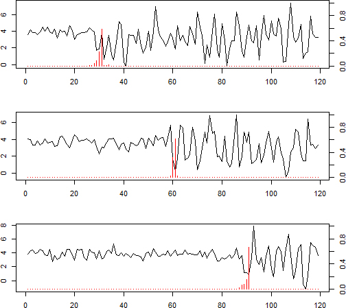$k_{1}$ .

As per discussion, the model is identified with help of the posterior probabilities. The posterior probabilities are recorded in Table 1. From Table 1, it is observed that Bayesian model probability is accurately identifying the data generating process (DGP) across for M4 model. The posterior probability of M4 is increased with increase the series size i.e., $T=200$ . Discarding the first 1,000 iterations as the burn-in period, the Gibbs sampler runs for 11,000 iterations, and the posterior mean and standard deviation are calculated. The hyper parameter values are $a=5$ and $b=0.5$ . The Bayes estimates and HPD intervals are calculated at 5% level of significance and recorded in Tables 2 and 3, respectively. For comparisons in different estimators, we also report average absolute bias (AB) and mean squared error (MSE) and shown in Table 4.

Table 2

Posterior mean (standard deviation) of M4 model parameter when $T=120$

$T,k_{1}$	Estimator	$\theta_{1}=0.1$	$\beta_{11}=0.2$	$\sigma_{1}^{2}=0.25$	$\theta_{2}=3.0$	$\beta_{21}=0.3$	$\beta_{22}=-0.3$	$\sigma_{2}^{2}=3.0$
120, 30	MLE	0.1061	0.1627	0.2482	3.0538	0.2877	$-$ 0.3084	2.9893
		( $-$ 0.1005)	( $-$ 0.1771)	( $-$ 0.0673)	( $-$ 0.4317)	( $-$ 0.1014)	( $-$ 0.0990)	( $-$ 0.4488)
	SELF	0.1059	0.1679	0.2513	3.0511	0.288	$-$ 0.308	2.9711
		( $-$ 0.0986)	( $-$ 0.1545)	( $-$ 0.0520)	( $-$ 0.4114)	( $-$ 0.0992)	( $-$ 0.0968)	( $-$ 0.4029)
	ABS	0.1014	0.1717	0.2374	3.0202	0.288	$-$ 0.3083	2.8448
		( $-$ 0.0986)	( $-$ 0.1546)	( $-$ 0.0501)	( $-$ 0.4108)	( $-$ 0.0993)	( $-$ 0.0968)	( $-$ 0.4070)
120, 60	MLE	0.103	0.1771	0.252	3.1101	0.2842	$-$ 0.3178	3.009
		( $-$ 0.0687)	( $-$ 0.1250)	( $-$ 0.0445)	( $-$ 0.5408)	( $-$ 0.1331)	( $-$ 0.1232)	( $-$ 0.5637)
	SELF	0.1031	0.1786	0.2527	3.1009	0.2855	$-$ 0.3166	2.9538
		( $-$ 0.0684)	( $-$ 0.1171)	( $-$ 0.0392)	( $-$ 0.4984)	( $-$ 0.1283)	( $-$ 0.1193)	( $-$ 0.4735)
	ABS	0.1	0.1821	0.245	3.0753	0.2828	$-$ 0.3198	2.7833
		( $-$ 0.0684)	( $-$ 0.1172)	( $-$ 0.0382)	( $-$ 0.4987)	( $-$ 0.1283)	( $-$ 0.1193)	( $-$ 0.4817)
120, 90	MLE	0.1042	0.1809	0.2495	3.1621	0.2701	$-$ 0.3263	3.0212
		( $-$ 0.0541)	( $-$ 0.0976)	( $-$ 0.0377)	( $-$ 0.7498)	( $-$ 0.1898)	( $-$ 0.1712)	( $-$ 0.8155)
	SELF	0.1043	0.1818	0.2502	3.1216	0.2759	$-$ 0.3206	2.7791
		( $-$ 0.054)	( $-$ 0.0933)	( $-$ 0.0345)	( $-$ 0.6311)	( $-$ 0.1759)	( $-$ 0.1614)	( $-$ 0.5795)
	ABS	0.1046	0.1836	0.2437	3.0968	0.2793	$-$ 0.3301	2.483
		( $-$ 0.054)	( $-$ 0.0934)	( $-$ 0.0342)	( $-$ 0.6321)	( $-$ 0.1763)	( $-$ 0.1614)	( $-$ 0.5912)

Table 3

Confidence interval and HPD interval of M4 model parameters when $T=120$

$T$ , $k_{1}$		MLE		SELF		ABS
		2.50%	97.50%	2.50%	97.50%	2.50%	97.50%
120, 30	$\theta_{1}$	$-$ 0.0665	0.3185	$-$ 0.0691	0.3050	$-$ 0.0661	0.3084
	$\beta_{11}$	$-$ 0.2072	0.4750	$-$ 0.1513	0.4432	$-$ 0.1552	0.4361
	$\sigma_{1}^{2}$	0.1353	0.3942	0.1626	0.3643	0.1573	0.3518
	$\theta_{2}$	2.2127	3.8610	2.2766	3.8596	2.2233	3.8102
	$\beta_{21}$	0.1010	0.5020	0.1035	0.4942	0.1009	0.4917
	$\beta_{22}$	$-$ 0.5237	$-$ 0.1324	$-$ 0.5264	$-$ 0.1466	$-$ 0.5276	$-$ 0.1466
	$\sigma_{2}^{2}$	2.0280	3.7872	2.2021	3.7740	2.0517	3.6354
	$\theta_{1}$	$-$ 0.0203	0.2466	$-$ 0.0178	0.2476	$-$ 0.0182	0.2467
	$\beta_{11}$	$-$ 0.0694	0.4127	$-$ 0.0508	0.4004	$-$ 0.0488	0.4010
	$\sigma_{1}^{2}$	0.1685	0.3384	0.1795	0.3286	0.1753	0.3216
120, 60	$\theta_{2}$	2.0510	4.1600	2.1038	4.0438	2.1907	4.1268
	$\beta_{21}$	$-$ 0.0215	0.5201	0.0553	0.5763	0.0499	0.5719
	$\beta_{22}$	$-$ 0.5452	$-$ 0.0769	$-$ 0.5417	$-$ 0.0871	$-$ 0.5412	$-$ 0.0859
	$\sigma_{2}^{2}$	1.8829	4.0415	2.1412	3.9538	1.8530	3.6954
	$\theta_{1}$	$-$ 0.0017	0.2104	$-$ 0.0014	0.2108	$-$ 0.0020	0.2102
	$\beta_{11}$	$-$ 0.0145	0.3589	$-$ 0.0086	0.3503	$-$ 0.0046	0.3538
	$\sigma_{1}^{2}$	0.1770	0.3231	0.1823	0.3146	0.1804	0.3105
120, 90	$\theta_{2}$	1.8541	4.6616	1.9797	4.3163	1.9579	4.3056
	$\beta_{21}$	$-$ 0.1396	0.6174	$-$ 0.0838	0.6104	$-$ 0.0860	0.6101
	$\beta_{22}$	$-$ 0.6508	$-$ 0.0120	$-$ 0.6161	$-$ 0.0138	$-$ 0.6153	$-$ 0.0136
	$\sigma_{2}^{2}$	1.6466	4.6942	1.7588	3.9550	1.5240	3.7612

Table 4

Average absolute bias and mean squared error of M4 model parameter when $T=120$

$T,k_{1}$		Average absolute bias
		$\theta_{1}$	$\beta_{11}$	$\sigma_{1}^{2}$	$\theta_{2}$	$\beta_{21}$	$\beta_{22}$	$\sigma_{2}^{2}$
120, 30	MLE	0.077	0.144	0.054	0.342	0.082	0.080	0.357
	SELF	0.076	0.126	0.041	0.325	0.080	0.078	0.322
	ABS	0.077	0.126	0.041	0.325	0.081	0.078	0.345
120, 60	MLE	0.055	0.101	0.035	0.437	0.107	0.100	0.453
	SELF	0.055	0.094	0.031	0.404	0.103	0.097	0.383
	ABS	0.054	0.094	0.031	0.404	0.103	0.097	0.424
120, 90	MLE	0.043	0.079	0.030	0.608	0.152	0.140	0.640
	SELF	0.043	0.076	0.027	0.514	0.141	0.132	0.507
	ABS	0.043	0.076	0.027	0.515	0.141	0.132	0.641
	Mean squared error
120, 30	MLE	0.010	0.033	0.005	0.189	0.010	0.010	0.201
	SELF	0.010	0.025	0.003	0.172	0.010	0.009	0.163
	ABS	0.010	0.025	0.003	0.171	0.010	0.009	0.183
120, 60	MLE	0.005	0.016	0.002	0.304	0.018	0.016	0.318
	SELF	0.005	0.014	0.002	0.258	0.017	0.015	0.226
	ABS	0.005	0.014	0.002	0.259	0.017	0.015	0.271
120, 90	MLE	0.003	0.010	0.001	0.588	0.037	0.030	0.665
	SELF	0.003	0.009	0.001	0.413	0.032	0.027	0.384
	ABS	0.003	0.009	0.001	0.414	0.032	0.027	0.575

Studying the results, one can observe that the AB and MSE of all estimators with different break points decrease as size of the time series is increased. Bayes estimator’s performance is better than the MLE. However, Bayes estimators obtained under SELF and ABS have shown similar performances. The simulation study is also analyzed for other models M1–M3 as well as different sizes of the series. But due to page limits, this is not included in main manuscript and provided as per need.

5. Empirical analysis

In this section, we apply our proposed methodology to illustrate real life applications and consider an empirical application of time series data on import and export prices of U.S. natural gas. Natural gas is taken as an energy source as the ideal transition fuel among traditional fossil fuels, coal and oil, and it is renewable for the future. With increasing concerns about the environmental and climate changes, consequence of greenhouse gas emissions, natural gas is heralded as a less harmful energy source. So, every nation wants to develop natural gas as an alternative resource. This is popular as a source of heating and cooking power in private residences as well as businesses purpose in most of the countries. The average price of the import and export natural gas was recorded in dollars per thousand cubic feet. Due to varying the natural gas price, there may be change in the structure of the time series. This variation may be explained with our proposed model.

5.1 Natural gas price of import series

For analysis purpose, the natural gas price of the import monthly series from 2001:1 to 2017:10 obtained from U.S. Energy Information Administration (EIA) which bears the structural break on all parameters including order. In order to identification of order change points, 10% data is trimmed. The posterior probability helps to identify the break point where the order is changed. The original series with posterior probability corresponding to each point is shown in Fig. 2.

In Fig. 2, we observed that there are two different regions where posterior probability of the break point forms a cluster. Considering more generalized view, we have considered one by one break point of the cluster as order change point and then fit the model. For simplicity, we consider maximum lag five of AR and get twenty combinations. In Fig. 2, highest probability recorded at break points Feb 2003 and Jan 2015, which lies between 1 ${}^{\text{st}}$ and 9 ${}^{\text{th}}$ deciles and M1 model has recorded the maximum probability value 0.99 and 0.98 for the change point locations at Feb 2003 and Jan 2015, respectively. So, we conclude that there only order change and no break on other parameters which shows that import series is not shifted due to intercept or/and error variance. The model coefficients value, mean squared error and AIC values are recorded in Table 5. In Table 5, it is observed that AIC and MSE is lesser corresponding to change point is present at January 2015.

Table 5
Model coefficient of the best order change model for import series onsidering single break

$k_{1}$	Estimator	$\theta$	$\beta_{11}$	$\beta_{21}$	$\beta_{22}$	$\sigma^{2}$	MSE	AIC
Feb 2003	MLE	0.900	0.779	1.103	$-$ 0.166	1.614	1.644	676.283
	SELF	0.885	0.722	1.033	$-$ 0.212	1.595	1.261	622.995
	ABS	0.885	0.721	1.032	$-$ 0.213	1.558	1.261	622.990
Jan 2015	MLE	0.648	1.281	$-$ 0.281	0.766	0.854	0.899	552.349
	SELF	0.727	1.200	$-$ 0.332	0.675	0.899	0.515	440.779
	ABS	0.730	1.201	$-$ 0.332	0.674	0.879	0.515	440.852

If we consider both order change points jointly and then search the best autoregressive model for each region. In order to construction of order combination for three regions, we get 125 different pairs. For each pair, we calculate the model probability for all four models and AIC values. The M2 model has maximum probability as compare to other three models and recorded pair has minimum AIC value for $p_{1}=1,p_{2}=2$ and $p_{3}=1$ . The coefficients of the M2 model and MSE are recorded in Table 6.

Table 6

Model coefficient of the best order change model for import series onsidering two breaks

Order ( $p_{1}$ , $p_{2}$ , $p_{3}$ )		$\theta_{1}$	$\beta_{11}$	$\beta_{12}$	$\theta_{2}$	$\beta_{21}$	$\theta_{3}$	$\beta_{31}$	$\sigma^{2}$	MSE	AIC
(2, 1, 1)	MLE	0.373	1.277	$-$ 0.259	0.478	0.972	0.754	0.763	0.658	0.635	486.670
	SELF	1.251	0.780	$-$ 0.108	0.662	0.886	1.054	0.603	1.137	0.536	452.999
	ABS	1.256	0.780	$-$ 0.106	0.660	0.886	1.051	0.604	1.087	0.537	453.041

The import series $({y_{t}})$ and fitted value are plotted in Fig. 3 and observed that SELF estimate gives good fit as compared to ABS and MLE estimate, since MSE and AIC values are smaller. In general, for one break and two breaks models, M2 model has minimum AIC and MSE. This model is may become more suitable for prediction of future spot price of the import natural gas and defiantly such type of analysis is helpful for making proper decision and to find a periodical strategic path in this sector.

Figure 2.

Spot price of the imported natural gas series with posterior probability of the breaks.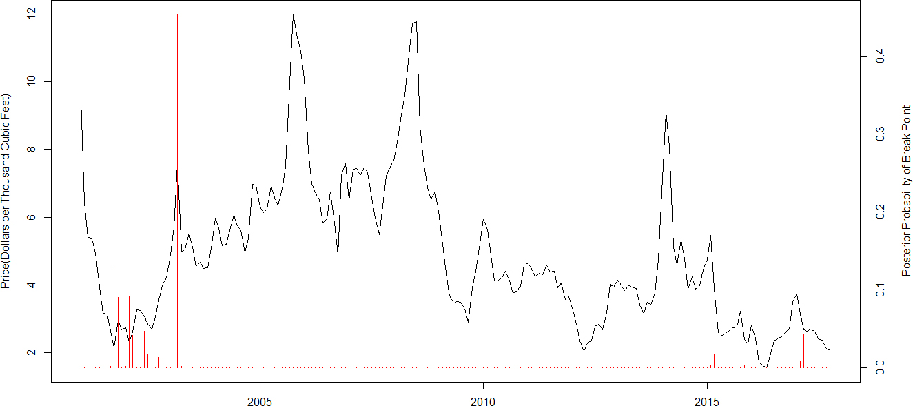

Figure 3.

Fitted series of the imported natural gas series when considering two breaks at Feb 2003 and Jan 2015.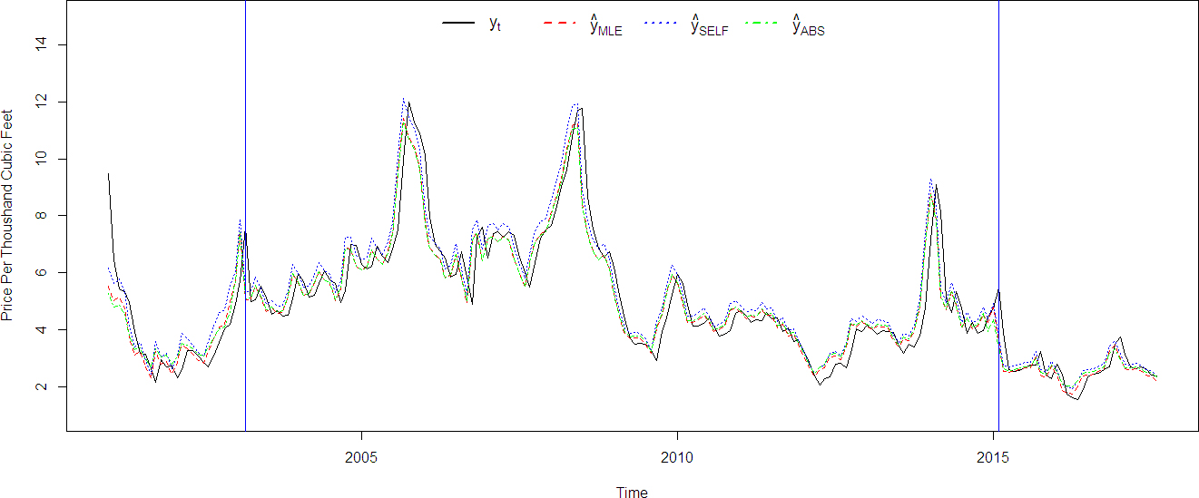

5.2 Natural gas price of export series

Similarly, we do the modelling of the export series and identify the order change points using the posterior probability. The export time series and posterior probability are shown in Fig. 4. After trimmed 10% series, we see that the first quarter of 2014 has the largest posterior probability as compared to rest of the points as shown in Fig. 4, which indicates that in this period order change phenomenon takes place.

Figure 4.

Spot price of the export natural gas series with posterior probability of breaks.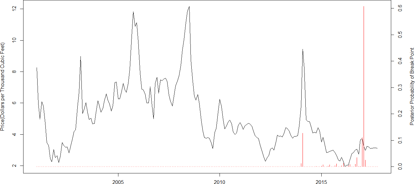

All three months of the first quarter are considered as an order change points and models are fitted. The best model is selected with the help of information criterion and posterior probability. The model posterior probability of the export series is recorded at change points Jan 2014, Feb 2014 and March 2014 with corresponding maximum probability values are 0.992, 0.996 and 0.992 respectively. Among all four models, M1 model has recorded the maximum probability. Thus, only order change model is suitable for export series also. The estimated coefficients, MSE and AIC value of M1 model corresponding to all three possible break points are recorded in Table 7 and observe that MSE and AIC values is minimum when March 2014 is considered as order change point with order (2, 5). The export time series and fitted series are plotted in Fig. 5. In this figure, SELF and ABS estimate give better fit as compared to MLE estimate.

Table 7

Model coefficient of the best order change model for export series

$k_{1}$		$\theta_{1}$	$\beta_{11}$	$\beta_{12}$	$\beta_{21}$	$\beta_{22}$	$\beta_{23}$	$\beta_{24}$	$\beta_{25}$	$\sigma^{2}$	MSE	AIC
Jan, 2014	MLE	0.638	1.187	$-$ 0.180	0.796	$-$ 0.288	0.454	$-$ 0.092	0.199	1.288	1.344	632.644
	SELF	0.685	1.113	$-$ 0.232	0.677	$-$ 0.239	0.301	$-$ 0.079	0.113	1.398	0.703	502.969
	ABS	0.684	1.110	$-$ 0.230	0.678	$-$ 0.239	0.300	$-$ 0.074	0.110	1.372	0.703	502.988
Feb, 2014	MLE	0.668	1.228	$-$ 0.223	0.632	$-$ 0.122	0.366	$-$ 0.055	0.204	1.188	1.247	617.658
	SELF	0.734	1.148	$-$ 0.272	0.529	$-$ 0.106	0.238	$-$ 0.056	0.121	1.306	0.611	474.901
	ABS	0.741	1.149	$-$ 0.272	0.529	$-$ 0.110	0.238	$-$ 0.053	0.122	1.272	0.611	475.050
Mar, 2014	MLE	0.712	1.164	$-$ 0.169	0.419	0.022	0.338	$-$ 0.015	0.217	1.122	1.182	607.060
	SELF	0.784	1.089	$-$ 0.223	0.331	0.018	0.223	$-$ 0.025	0.132	1.230	0.550	454.097
	ABS	0.779	1.089	$-$ 0.222	0.330	0.017	0.225	$-$ 0.025	0.134	1.202	0.550	454.074

Figure 5.

Fitted series of the export natural gas series when considering a break at March 2014.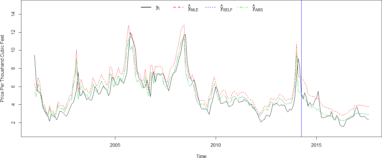

6. Conclusion

Time series modelling is a special approach of modelling where present states are dependent on it’s past. In this article, a times series model is proposed which allows the break on autoregressive coefficients, error variance as well as order of dependence in case of autoregressive time series. The estimation methodologies such as maximum likelihood and Bayesian estimations with squared error and absolute loss functions are discussed for estimating the parameters of the proposed model. The simulation study is carried out to compare the performances of the estimators. The proposed model is also trained for U.S. natural gas price of import and export time series for empirical example. Study recorded the two breaks in import series on Feb 2003 and Jan 2015. However, in export series order change phenomenon is happened in 1st quarter. The best model was identified corresponding to minimum AIC as well as maximum posterior probability. As the model is very less explored so this may also train for model selection based on accuracy of forecasting. The present work may be extended in case of multivariate time series and time series model with non-normal error in future work.

Footnotes

Appendix

Table A1

Posterior mean and variance of the parameters of the model M1–M4

Model		Distribution	Mean	Variance
M1	$\beta_{i}$	Multivariate Normal	$({X_{i}^{\prime}({Y_{i}-\theta l_{n_{i}}})+I_{p_{i}}^{-1}\mu_{i}})^{\prime}({X% _{i}^{\prime}X_{i}+I_{p_{i}}^{-1}})^{-1}$	$({X_{i}^{\prime}X_{i}+I_{p_{i}}^{-1}})^{-1}\sigma^{2}$
	$\theta$	Normal	$({\sum_{i=0}^{N_{T}}{({Y_{i}-\beta_{i}X_{i}})^{\prime}l_{n_{i}}}+\delta})({% \sum_{i=0}^{N_{T}}{l_{n_{i}}^{\prime}l_{n_{i}}}+1})^{-1}$	$({\sum_{i=0}^{N_{T}}{l_{n_{i}}^{\prime}l_{n_{i}}}+1})^{-1}\sigma^{2}$
	$\sigma^{2}$	Inverse Gamma	$\frac{D_{1}}{T+\sum_{i=0}^{N_{T}}{p_{i}}+2a-1}$	$\frac{V_{1}^{2}}{({T+\sum_{i=0}^{N_{T}}{p_{i}}+2a-1})^{2}({T+\sum_{i=0}^{N_{T}% }{p_{i}}+2a-3})}$
M2	$\beta_{i}$	Multivariate Normal	$({X_{i}^{\prime}({Y_{i}-\theta l_{n_{i}}})+I_{p_{i}}^{-1}\mu_{i}})^{\prime}({X% _{i}^{\prime}X_{i}+I_{p_{i}}^{-1}})^{-1}$	$({X_{i}^{\prime}X_{i}+I_{p_{i}}^{-1}})^{-1}\sigma^{2}$
	$\theta_{i}$	Normal	$({({Y_{i}-\beta_{i}X_{i}})^{\prime}l_{n_{i}}+\delta_{i}})({l_{{}_{n_{i}}}^{% \prime}l_{n_{i}}+1})^{-1}$	$({l_{{}_{n_{i}}}^{\prime}l_{n_{i}}+1})^{-1}\sigma^{2}$
	$\sigma^{2}$	Inverse Gamma	$\frac{D_{2}}{T+\sum_{i=0}^{N_{T}}{p_{i}}+N_{T}+2a-1}$	$\frac{V_{2}^{2}}{({T+\sum_{i=0}^{N_{T}}{p_{i}}+N_{T}+2a-1})^{2}({T+\sum_{i=0}^% {N_{T}}{p_{i}}+N_{T}+2a-3})}$
M3	$\beta_{i}$	Multivariate Normal	$({X_{i}^{\prime}({Y_{i}-\theta l_{n_{i}}})+I_{p_{i}}^{-1}\mu_{i}})^{\prime}({X% _{i}^{\prime}X_{i}+I_{p_{i}}^{-1}})^{-1}$	$({X_{i}^{\prime}X_{i}+I_{p_{i}}^{-1}})^{-1}\sigma^{2}$
	$\theta$	Normal	$({\sum_{i=0}^{N_{T}}{\frac{({Y_{i}-\beta_{i}X_{i}})^{\prime}l_{n_{i}}}{\sigma_% {i}^{2}}}+\frac{\delta}{\tau}})({\sum_{i=0}^{N_{T}}{\frac{l_{{}_{n_{i}}}^{% \prime}l_{n_{i}}}{\sigma_{i}^{2}}}+\frac{1}{\tau}})^{-1}$	$({\sum_{i=0}^{N_{T}}{\frac{l_{{}_{n_{i}}}^{\prime}l_{n_{i}}}{\sigma_{i}^{2}}}+% \frac{1}{\tau}})^{-1}$
	$\sigma_{i}^{2}$	Inverse Gamma	$\frac{D_{3i}}{p_{i}+n_{i}+2a-2}$	$\frac{V_{3i}^{2}}{({p_{i}+n_{i}+2a-2})^{2}({p_{i}+n_{i}+2a-4})}$
M4	$\beta_{i}$	Multivariate Normal	$({X_{i}^{\prime}({Y_{i}-\theta l_{n_{i}}})+I_{p_{i}}^{-1}\mu_{i}})^{\prime}({X% _{i}^{\prime}X_{i}+I_{p_{i}}^{-1}})^{-1}$	$({X_{i}^{\prime}X_{i}+I_{p_{i}}^{-1}})^{-1}\sigma^{2}$
	$\theta_{i}$	Normal	$({({Y_{i}-\beta_{i}X_{i}})^{\prime}l_{n_{i}}+\delta_{i}})({l_{{}_{n_{i}}}^{% \prime}l_{n_{i}}+1})^{-1}$	$({l_{{}_{n_{i}}}^{\prime}l_{n_{i}}+1})^{-1}\sigma^{2}$
	$\sigma_{i}^{2}$	Inverse Gamma	$\frac{D_{4i}}{n_{i}+p_{i}+2a-1}$	$\frac{V_{4i}^{2}}{({n_{i}+p_{i}+2a-1})^{2}({n_{i}+p_{i}+2a-3})}$

References

Bai

(2010). Common breaks in means and variances for panel data. Journal of Econometrics, 157(1), 78-92.

Barbieri

M. M.

, & Conigliani

(1998). Bayesian analysis of autoregressive time series with change points. Journal of the Italian Statistical Society, 7(3), 243-255.

Broemeling

L. D.

(1972). Bayesian procedures for detecting a change in a sequence of random variables. Metron, 30, 1-14.

Chaturvedi

, & Kumar

(2007). Bayesian unit root test for time series models with structural breaks. American Journal of Mathematical and Management Sciences, 27(1-2), 243-268.

Chib

(1998). Estimation and comparison of multiple change-point models. Journal of Econometrics, 86(2), 221-241.

Cook

(2001). Asymmetric unit root tests in the presence of structural breaks under the null. Economics Bulletin, 3(6), 1-10.

(2016). Structural changes in inflation dynamics: multiple breaks at different dates for different parameters. Studies in Nonlinear Dynamics & Econometrics, 20(3), 211-231.

Geman

, & Geman

(1984). Stochastic relaxation, Gibbs distribution and the Bayesian restoration of images. IEEE Transactions on Pattern Analysis and Machine Intelligence, 6, 721-741.

Inclan

(1993). Detection of multiple changes of variance using posterior odds. Journal of Business & Economic Statistics, 11(3), 289-300.

10.

Kezim

, & Abdelli

(2004). A Bayesian analysis of a structural change in the parameters of a time series. Communications in Statistics-Theory and Methods, 33(8), 1863-1876.

11.

Kim

(1991). A Bayesian significance test of the stationarity of regression parameters. Biometrika, 78(3), 667-675.

12.

Kim

T. H.

Leybourne

, & Newbold

(2002). Unit root tests with a break in innovation variance. Journal of Econometrics, 109(2), 365-387.

13.

Kumar

, & Chaturvedi

(2012). Bayesian unit root test for time series models with structural break in variance. Journal of Economics and Econometrics, 55(1), 75-86.

14.

Lee

, & Strazicich

M. C.

(2003). Minimum Lagrange multiplier unit root test with two structural breaks. Review of Economics and Statistics, 85(4), 1082-1089.

15.

Maddala

G. S.

, & Kim

I. M.

(1998). Unit roots, cointegration and structural change (No. 4). Cambridge University Press.

16.

Meligkotsidou

Tzavalis

, & Vrontos

I. D.

(2011). A Bayesian analysis of unit roots and structural breaks in the level, trend and error variance of autoregressive models of economic series. Econometric Reviews, 30(2), 208-249.

17.

Meligkotsidou

Tzavalis

, & Vrontos

I. D.

(2017). On Bayesian analysis and unit root testing for autoregressive models in the presence of multiple structural breaks. Econometrics and Statistics, 4, 70-90.

18.

Perron

(1990). Testing for a unit root in a time series with a changing mean. Journal of Business & Economic Statistics, 8(2), 153-162.

19.

Perron

, & Vogelsang

T. J.

(1992). Nonstationarity and level shifts with an application to purchasing power parity. Journal of Business & Economic Statistics, 10(3), 301-320.

20.

Shao

, & Zhang

(2010). Testing for change points in time series. Journal of the American Statistical Association, 105(491), 1228-1240.

21.

Slama

, & Saggou

(2017). A Bayesian analysis of a change in the parameters of autoregressive time series. Communications in Statistics-Simulation and Computation, 46(9), 7008-7021.

22.

Smith

A. F. M.

(1975). A Bayesian approach to inference about a change-point in a sequence of random variables. Biometrika, 62(2), 407-416.

23.

Vosseler

(2016). Bayesian model selection for unit root testing with multiple structural breaks. Computational Statistics & Data Analysis, 100, 616-630.

24.

Wang

, & Zivot

(2000). A Bayesian time series model of multiple structural changes in level, trend and variance. Journal of Business & Economic Statistics, 18(3), 374-386.

25.

Zivot

, & Andrews

D. W. K.

(1992). Further evidence on the great crash, the oil-price shock and the unit-root hypothesis. Journal of Business & Economic Statistics, 10(3), 251-270.