A binary choice model with partial observability for panel data

Abstract

We consider a panel model with a binary response variable that is a product of two unobservable factors, each determined by a separate binary choice equation. One of these factors is assumed to be time-invariant and may be interpreted as a latent class indicator. A simulation study shows that maximum likelihood estimates from even the shortest panel are much more reliable than those obtained from a cross-section. As an illustrative example, the model is applied to Russian Longitudinal Monitoring Survey data to estimate a proportion of the non-employed population who are participating in job search.

Keywords

Partial observability split population binary choice latent classes

1. Introduction

Event history analysts and survival statisticians are familiar with problems that require treating data as a sample drawn from a heterogeneous population split into two latent classes. The first class consists of objects that are going to face a certain event of interest sooner or later, while the second class includes those objects that never face the event. Models that allow for such heterogeneity are known as cure models in medicine (Boag, 1949) and split-population or mover-stayer models in event-history analysis (Schmidt & Witte, 1989; Blumen et al., 1955; Yamaguchi, 2003). Poirier (1980) used a similar approach when introducing a partial observability model for binary choice.

In this paper, we propose a panel version of a partial observability model and show that panel data allow the identification of parameters that are unidentified in the cross-section case. The paper is organized as follows. Section 2 contains a brief review of research concerning partial observability models and their applications. Section 3 describes in detail the model with partially observable bivariate binary response for cross-sectional data. Section 4 presents the extended version of the model for use with panel data. Section 5 contains the results of a simulation study. Section 6 gives an example of the model’s application to the job search analysis. Section 7 concludes the article.

2. Literature review

Binary choice models with partial observability were introduced by Poirier (1980) who gives an example from a study on the retention of trainees (Gunderson, 1974): a researcher knows whether a trainee continues working after the completion of training, but this choice is not just an individual decision. The trainee cannot continue working if the employer decides not to retain him. Therefore, we may consider a latent class of individuals who are able both to continue working and to quit and another latent class for those who have no choice except to quit the job because the employer is not interested in retaining them. Poirier uses the term “partial observability” because in this situation, a researcher does not observe the individual decisions of the trainee and the employer but only the result determined by both decisions. Poirier considers a model that consists of two probit equations for unobserved factors (decisions of the trainee and the employer) and the only observed dependent variable which is the product of these factors. Although the paper starts with demonstrative example from labor economics, it is purely theoretical and deals mostly with identifiability issues.

Applications of partial observability models include the study of political interactions by Nieman (2015), where a civil war onset is explained by unobserved decisions of rebels and the government, similar studies on international relations and conflicts (Signorino, 1999, 2002) and works on misreporting in survey data (Beger et al., 2011; Rainey & Jackson, 2013).

Identifiability of models’ parameters and reliability of estimates in presence of partial observability have always been the issue of concern. Simulation studies were conducted to examine statistical properties of estimators but these studies led to substantially different conclusions. The results presented in Beger et al. (2011) show that the estimates agree with true values, while Rainey and Jackson (2017) found the inference from partial observability models to be seriously misleading. Nieman (2015) investigates the consequences of misspecification and concludes that the estimates from misspecified models are biased but nonetheless useful. Rainey and Jackson (2017) state that even a slight specification error leads to substantial bias and distorts results of significance tests.

3. Bivariate binary model with partial observability: Cross-sectional data

For the sake of convenience, let us return to the example with the retention of trainees and consider a sample that consists of $n$ independent observations. Let $x_{i}^{\prime}$ be a row vector of variables that determine the trainee’s decision $y_{1,i}$ ( $y_{1,i}=1$ if the trainee wants to continue working, and $y_{1,i}=0$ if he or she wants to quit), and $z_{i}^{\prime}$ be a row vector of variables that determine the employer’s decision $y_{2,i}$ in observation $i$ ( $y_{2,i}=1$ if the employer decides to retain the worker, and $y_{2,i}=0$ otherwise). We do not know each agent’s decision and observe only the variable $y_{i}=y_{1,i}y_{2,i}$ , which equals 1 when the trainee continues working and 0 when the trainee quits, either voluntarily or due to the employer.

The probabilities of the agents’ decisions are

$\displaystyle P(y_{1,i}=1)=F(x_{i}^{\prime}\beta),$ (1) $\displaystyle P(y_{2,i}=1)=G(z_{i}^{\prime}\gamma).$ (2)

Here, $\beta$ and $\gamma$ denote vectors of the coefficients to be estimated, and $F(x)$ and $G(x)$ are increasing functions that take values from 0 to 1. Poirier (1980) considers the case

$\displaystyle F(x)=G(x)=\frac{1}{\sqrt{2\pi}}\int_{-\infty}^{x}{\exp(-{u^{2}}/% 2){\rm d}u}.$ (3)

In this case, the decisions of both the trainee and employer are determined by probit equations. The split-population logit model presented in Beger et al. (2011) is similar but uses a logistic function for $F(x)$ and $G(x)$ .

If variables $y_{1,1},\ldots,y_{1,n},y_{2,1},\ldots,y_{2,n}$ are assumed to be independent, then the probability of retention is

$\displaystyle P(y_{i}=1)=F(x_{i}^{\prime}\beta)G(z_{i}^{\prime}\gamma).$ (4)

The specification used by Poirier allows for correlation between the agents’ decisions, but we do not consider that case, nor do Beger et al. (2011); Nieman (2015); Rainey and Jackson (2013, 2017).

Coefficient vectors $\beta$ and $\gamma$ are estimated by maximizing the log-likelihood function:

$\displaystyle\ln L(y_{1},\ldots,y_{\rm n};x_{1}^{\prime},\ldots,x_{\rm n}^{% \prime};z_{1}^{\prime},\ldots,z_{\rm n}^{\prime};\beta,\gamma)$ $\displaystyle=\sum_{i=1}^{n}[y_{i}(\ln F(x_{i}^{\prime}\beta)+\ln G(z_{i}^{% \prime}\gamma))+(1-y_{i})\ln(1-F(x_{i}^{\prime}\beta)G(z_{i}^{\prime}\gamma))]% \mathop{\to}\limits_{\beta,\gamma}\max.$ (5)

One problem that arises when dealing with such a model is possible nonidentifiability. The simplest example of the unidentified model is obtained by omitting all the explanatory variables so that $x_{i}^{\prime}\beta$ and $z_{i}^{\prime}\gamma$ reduce to scalars $\beta_{1}$ and $\gamma_{1}$ . Then, the log-likelihood depends only on $F(\beta_{1})G(\gamma_{1})$ but not on $\beta_{1}$ and $\gamma_{1}$ separately, so the parameters cannot be uniquely identified. Adding explanatory variables may help, but “identification in partially observed bivariate probit models is a somewhat tricky problem” (Poirier, 1980, p. 215). To a certain extent, that problem may be solved by using the Bayesian approach, although it is not an absolute remedy (Poirier, 1998).

Rainey and Jackson (2017) note another weak point: estimates obtained from partial observability models are highly sensitive to misspecification. Choosing wrong functions $F(x)$ and $G(x)$ not only brings substantial bias to the estimates but also may reverse their signs. Although this result is worthy of attention, it may not be as discouraging as it seems. The question is: what are the “real” parameter values in the misspecified model? Biased estimates may not only provide a better fit to the data but also yield better out-of-sample predictions than even true parameters when they are put into a wrong function.

Most researchers, however, are interested not in predictions but in explanatory ability or theoretical inference, and switching the coefficient sign means providing the opposite explanation of a phenomenon under study. It seems that the results of Rainey and Jackson simply remind us that there can be empirically almost-equivalent models that contradict each other. This phenomenon is not just a drawback of partial observability models but a problem of science as a whole. Such a discussion is beyond the scope of our paper, although we consider it highly important. At the moment, however, let us conclude that consequences of misspecification are not as clear as they may seem.

4. Bivariate binary model with partial observability: Panel data

Now, we turn to a case where a sample consists of repeated observations of $n$ objects, so that object $i$ is observed $T_{i}$ times. Number of observations may vary from one object to another (the panel may be unbalanced). The observed response value $y_{it}$ for object $i$ in period $t$ is a product of two latent binary variables: $y_{it}=y_{1,it}y_{2,i}$ . Variables $y_{1,it}$ are linked to covariates $x_{it}^{\prime}$ by equation $P(y_{1,it}=1)=F(x_{it}^{\prime}\beta)$ . Variables $y_{2,i}$ and $i=1,\ldots,n$ are independent and time-invariant, and they depend on time-invariant covariates $z_{i}^{\prime}$ : $P(y_{2,i}=1)=G(z_{i}^{\prime}\gamma)$ .

We assume that all latent variables $y_{1,it}$ , $t=1,\ldots,T_{i}$ , $i=1,\ldots,n$ and $y_{2,i}$ , $i=1,\ldots,n$ are independent. However, the observed responses $y_{i1},\ldots,y_{iT_{i}}$ for each object $i$ are correlated because they include the same factor $y_{2,i}$ .

The response probabilities in a separate observation are determined by the following equation:

$\displaystyle P(y_{it}=1)=F(x_{it}^{\prime}\beta)G(z_{i}^{\prime}\gamma).$ (6)

The probability of observing values $y_{i1},\ldots,y_{iT_{i}}$ for object $i$ is

$\displaystyle L_{i}=G(z_{i}^{\prime}\gamma)\left[{\prod_{t=1}^{T_{i}}{F(x_{it}% ^{\prime}\beta)^{y_{it}}({1-F(x_{it}^{\prime}\beta)})^{1-y_{it}}}}\right]+(1-G% (z_{i}^{\prime}\gamma))\prod_{t=1}^{T_{i}}{({1-y_{it}})}.$ (7)

The log-likelihood function is obtained by summing the logs of these probabilities over all objects:

$\displaystyle\ln L=\sum_{i=1}^{n}{\ln L_{i}}.$ (8)

Maximizing the log-likelihood with respect to coefficient vectors $\beta$ and $\gamma$ gives us estimates for these coefficients.

It is rather weird to assume that the decision of one agent is time-invariant while another agent may change his mind, so this interpretation seems to be of little use. It is more appropriate to consider $y_{2,i}$ as a latent class indicator in the manner of automatic classification problems (Aivazian, 1987; Aivazian et al., 2015; Peresetsky et al., 2011) or mover-stayer processes (Blumen et al., 1955). If $y_{2,i}=0$ , then object $i$ belongs to a class of “stayers” that never change their state ( $y_{it}=0$ for each $t$ ). Objects with $y_{2,i}=1$ constitute a class of “movers” that switch between two possible states reflected by the observed response variable.

One may also think of time-invariant factors as individual effects. A common formulation for a binary choice model with individual effects $u_{i}$ is

$\displaystyle P(y_{it}=1)=F(x_{it}^{\prime}\beta+u_{i}).$ (9)

If we assume that $u_{i}$ are independent and normally distributed random variables uncorrelated with regressors $x_{it}$ , we obtain a random effects model. Assuming $u_{i}$ to be either nonstochastic or random but correlated with regressors leads to a fixed effects model (Hilbe, 2009). Our partial observability model is obtained when $u_{i}$ takes the value 0 with probability $G(z_{i}^{\prime}\gamma)$ and $-\infty$ with probability $1-G(z_{i}^{\prime}\gamma)$ . The individual effect may correlate with covariates $x_{it}^{\prime}$ because some variables may enter both vectors $x_{it}^{\prime}$ and $z_{i}^{\prime}$ . This specification may be considered an alternative to random and fixed effects.

5. Simulation study

We have conducted several simulation experiments to examine the properties of the estimators obtained by fitting the panel model with partial observability and its version for cross-sectional data. The results of one such experiment are presented below.

Data are generated according to the following system of equations:

$\displaystyle\begin{cases}x_{it}^{\prime}\beta=\beta_{1}+\beta_{2}x_{2,it}+% \beta_{3}x_{3,it},\\ z_{i}^{\prime}\gamma=\gamma_{1}+\gamma_{2}z_{2,i}+\gamma_{3}z_{3,i}.\end{cases}$ (10)

Both equations are specified as logit models: $F(x)=G(x)=\frac{\exp(x)}{1+\exp(x)}$ .

Values of random variables $x_{2,it}$ and $z_{2,i}$ are drawn from standard normal distribution, where $x_{3,it}$ takes values 0 and 1 with equal probabilities, and $z_{3,it}$ takes value 1 with probability 0.6 and 0 with probability 0.4. All the values are generated independently. Variables for the second equation are time-invariant (so there $i s$ dependence between response values $y_{1},\ldots,y_{\rm n}$ due to the time-invariant part $y_{2,1},\ldots,y_{2,n})$ . True parameter values are $\beta_{1}=0.2$ , $\beta_{2}=0$ , $\beta_{3}=0.4$ , $\gamma_{1}=0.3$ , $\gamma_{2}=0.6$ , and $\gamma_{3}=0$ .

Log-likelihood is maximized via the Newton-Raphson algorithm, and derivatives are calculated numerically (method d0 in Stata).

We generate 10,000 random samples for each pair $(n,T)$ , where $n\in\{200,500,1000\}$ is the number of objects and $T\in\{1,2,4\}$ is the number of time periods (which is the same for all objects in our experiment). The results are presented in Table 1. MAE denotes mean absolute error, MSE denotes mean squared error, and Prop. is the proportion of 95% confidence intervals covering true parameter values.

Table 1

Results of the simulation study

$n=$ 200, $T=$ 1, convergence achieved in 82.18% of cases
	$\hat{\beta}_{1}$	$\hat{\beta}_{2}$	$\hat{\beta}_{3}$	$\hat{\gamma}_{1}$	$\hat{\gamma}_{2}$	$\hat{\gamma}_{3}$
Bias	0.644	0.065	2.548	0.857	0.674	0.256
MAE	1.177	0.616	3.097	1.512	0.859	1.175
MSE	18.848	6.329	42.645	34.242	22.319	29.761
Prop.	0.841	0.973	0.976	0.778	0.926	0.975
$n=$ 200, $T=$ 2, convergence achieved in 100% of cases
Bias	$-$ 0.005	0.001	0.009	0.034	0.039	0.000
MAE	0.202	0.125	0.247	0.264	0.179	0.309
MSE	0.065	0.025	0.097	0.120	0.056	0.154
Prop.	0.951	0.951	0.951	0.964	0.955	0.957
$n=$ 200, $T=$ 4, convergence achieved in 100% of cases
Bias	$-$ 0.002	$-$ 0.001	0.004	0.007	0.019	0.002
MAE	0.113	0.079	0.158	0.199	0.138	0.255
MSE	0.020	0.010	0.039	0.063	0.031	0.103
Prop.	0.950	0.949	0.951	0.955	0.952	0.948
$n=$ 500, $T=$ 1, convergence achieved in 94.48% of cases
Bias	1.214	$-$ 0.358	2.298	0.352	0.276	0.026
MAE	1.689	0.738	2.583	0.984	0.433	0.428
MSE	4642.487	1212.197	119.066	2.902	0.768	1.149
Prop.	0.807	0.968	0.966	0.736	0.866	0.978
$n=$ 500, $T=$ 2, convergence achieved in 100% of cases
Bias	0.000	0.000	0.001	0.013	0.014	0.000
MAE	0.126	0.077	0.155	0.159	0.107	0.188
MSE	0.025	0.010	0.038	0.040	0.018	0.055
Prop.	0.949	0.952	0.948	0.954	0.951	0.954
$n=$ 500, $T=$ 4, convergence achieved in 100% of cases
Bias	0.002	0.000	0.001	0.002	0.007	0.001
MAE	0.071	0.050	0.100	0.121	0.085	0.157
MSE	0.008	0.004	0.016	0.023	0.011	0.039
Prop.	0.953	0.952	0.950	0.954	0.953	0.955
$n=$ 1000, $T=$ 1, convergence achieved in 98.14% of cases
Bias	0.578	0.041	2.168	0.078	0.107	$-$ 0.005
MAE	0.957	0.303	2.345	0.687	0.256	0.219
MSE	108.183	16.479	27.664	1.229	0.196	0.186
Prop.	0.724	0.971	0.963	0.735	0.794	0.975
$n=$ 1000, $T=$ 2, convergence achieved in 100% of cases
Bias	0.000	$-$ 0.001	0.001	0.006	0.007	$-$ 0.002
MAE	0.089	0.055	0.109	0.112	0.073	0.131
MSE	0.013	0.005	0.019	0.020	0.009	0.027
Prop.	0.947	0.950	0.949	0.955	0.952	0.955
$n=$ 1000, $T=$ 4, convergence achieved in 100% of cases
Bias	0.000	0.000	0.001	0.003	0.002	$-$ 0.002
MAE	0.050	0.035	0.070	0.088	0.060	0.113
MSE	0.004	0.002	0.008	0.012	0.006	0.020
Prop.	0.950	0.953	0.950	0.950	0.951	0.950

The maximization procedure fails to converge on some samples. This failure is quite common in a cross-section case, although the proportion of failures declines with sample size increasing. The panel data almost guarantee convergence. There were no failures in the described case, but in some other experiments with the same sample sizes, we observed a very small proportion of nonconvergences (less than 0.1%) when dealing with short panels, $T=2$ . Of course, one can intentionally generate data in a way that leads to a higher frequency of failures.

Nonconvergence takes place when the value of a parameter that maximizes the log-likelihood function is infinite. Such cases may appear even when estimating univariate binary choice models (“perfect separation”; see Hilbe (2009)). They also take place when a simple logit model fits the data better than a model with partial observability, so that a maximization procedure tries to set $G(z_{i}^{\prime}\gamma)=1$ by pushing the intercept term in $\gamma$ towards infinity.

The large MSEs in certain cells of Table 1 indicate that there might be some proportion of false convergences when the maximization procedure stopped at very large coefficient values because of numerical inaccuracy. In such cases, we also observe substantial bias and a proportion of correct confidence intervals that differ from the nominal confidence level.

We have tried to correct the simulation results by omitting estimates with implausibly high absolute values for at least one coefficient (for example, more than 100). Nevertheless, evidence for bias and incorrect inference does not disappear even after excluding all the cases with estimates greater than 10 in absolute value. Figure 1 presents a histogram with a kernel density plot for the remaining values of $\hat{\gamma}_{1}$ (7881 observations). The distribution is skewed and has a heavy right tail, the mean is 0.794, and the standard deviation is 1.292, so the bias persists. More than that, the estimated bias is even higher: 0.494 instead of 0.352 in Table 2. The proportion of correct 95% confidence intervals for $\gamma_{1}$ is 79.9%.

Figure 1.

Estimated density function for 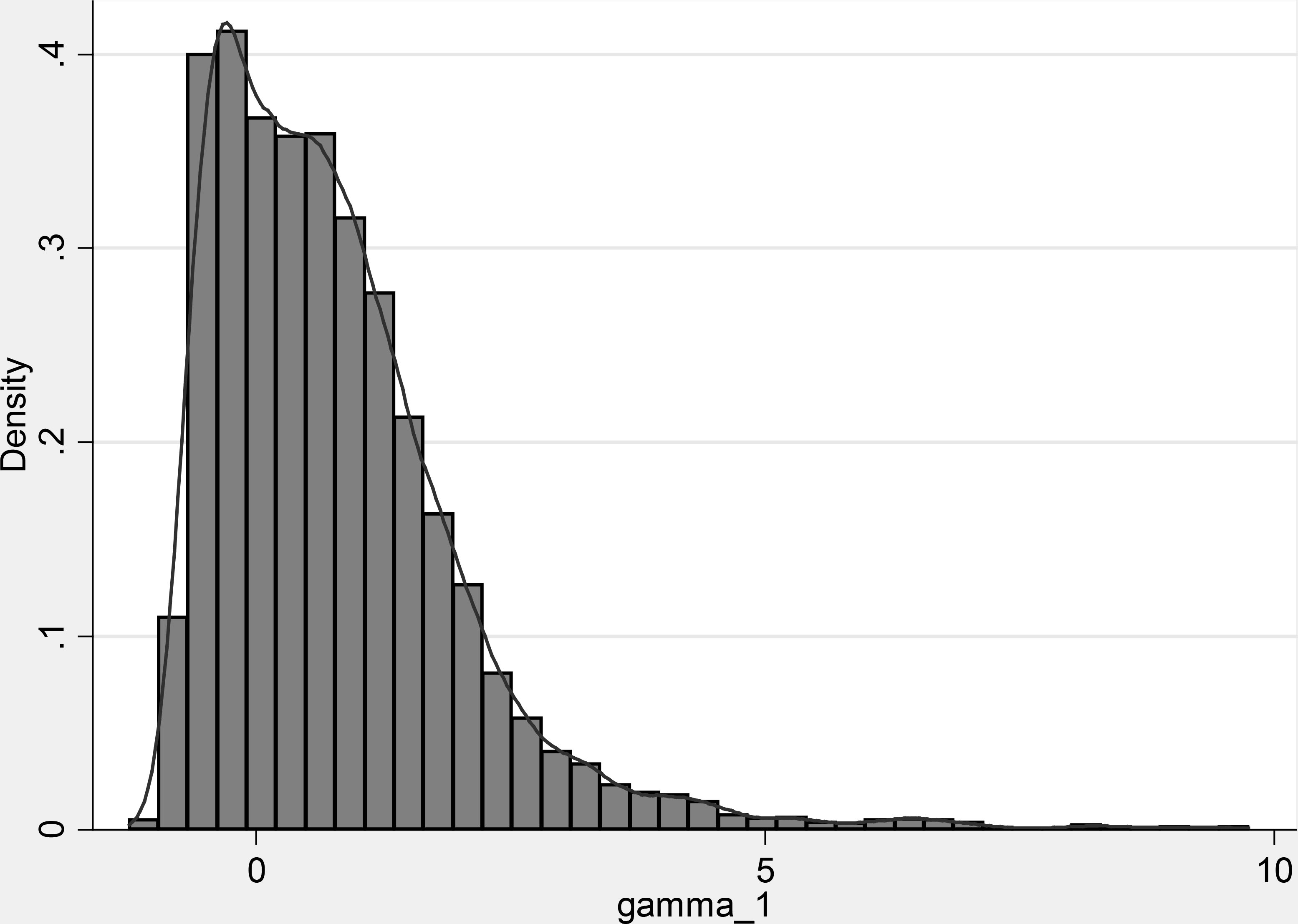$\hat{\gamma}_{1}$ ( $n=$ 500, $T=$ 1) after excluding observations with suspiciously large coefficient values.

It is worth describing other experiments in brief. They accounted for:

•

Correlation between explanatory variables with coefficient of correlation varying from 0 to 0.97;

•

Same covariates appearing in both equations;

•

No explanatory variables for time-invariant factor (only intercept term);

•

Covariates with normal and Bernoulli distribution with probabilities of values 0 and 1 ranging from 0.1 to 0.9;

•

Unbalanced panels with random number of observations per object.

We did not study the properties of estimators with almost perfectly correlated covariates or Bernoulli distributed explanatory variables with probabilities close to 0 or 1, so the caution should be taken when fitting the model in presence of multicollinearity.

All our experiments show that the use of panel data greatly reduces the proportion of nonconvergences, allowing for the estimation of parameters that would be unidentified in the cross-section case, and secures more reliable inferences.

6. Example: Job search among the non-employed in Russia

Consider a simple job search model described in Kiefer (1988). An agent is seeking a job and receives offers that he or she can either accept or reject. Once the agent accepts an offer, the job search ends, and the agent becomes employed. If acceptable offers arrive according to a Poisson process with intensity rate $\lambda$ , then the probability of finding a job within a unit of time is $p_{\text{find}}=1-\exp(-\lambda)$ .

Now let us introduce heterogeneity among the non-employed individuals: agents are involved in a job search with probability $p_{\text{search}}$ . Those who are not job seekers do not receive any offers and never enter employment. We know whether an agent has found a job during a certain time period but do not know whether he or she is a job seeker.

Let $y_{it}$ indicate whether an individual $i$ found a job during a time period $[t;t+1]$ ( $y_{it}=1$ for those who have found a job, and 0 otherwise). This variable can be expressed as the product of two latent factors: $y_{it}=y_{1,it}y_{2,i}$ , where $y_{1,it}$ indicates whether an agent would have found a job if he looked for it, and $y_{2,i}$ is 1 for job seekers and 0 otherwise.

The problem is to estimate probabilities of job search participation and of finding a job within a given period of time. It can be considered as a kind of classification problem for binary data (Aivazian et al., 2016).

We use the following parameterization (here, $\beta$ and $\gamma$ are scalars):

$\displaystyle P(y_{1,it}=1)=p_{\text{find}}=1-\exp(-\exp(\beta)),$ (11) $\displaystyle P(y_{2,i}=1)=p_{\text{search}}=\frac{\exp(\gamma)}{1+\exp(\gamma% )}.$ (12)

This is the panel model with partial observability from Section 3 with no covariates, where the first equation is the same as in a logit regression, and the second equation is the same as in a cloglog regression. Of course, other parameterizations lead to the same point estimates, although confidence intervals slightly differ.

The model is estimated from RLMS HSE data for the period from 2000 to 2015. The sample includes observations on non-employed men aged 18 to 59 years and women aged 18 to 54 years. We fit the model to two-year subpanels of men and women separately. Estimated probabilities of job search participation and proportions of job seekers are presented in Table 2. The table also presents pooled estimate for the probability of finding a job that is obtained under homogeneity assumption (all individuals are looking for job). Columns with observation numbers contain odd values because of attrition: some individuals were not observed for the full period. Untransformed estimates of $\beta$ and $\gamma$ along with their standard errors are given in Appendix.

The proportion of job seekers among both sexes mostly ranges between 50% and 65%, and men stably have a higher probability of successful search than women. We have also found that the estimated proportion of seekers increases when fitting the model to longer panels, which is quite natural. For example, using data from the 2000–2008 period, we obtain practically equal values of 89.4% and 89.5% for the proportion of seekers among men and women, respectively.

Table 2

Proportion of job seekers ( $p_{\text{search}}$ ), probability that a seeker would find a job within a year ( $p_{\text{find}}$ ) and pooled estimate for the probability of transition to employment ( $p_{\text{pooled}}$ ); estimates from RLMS HSE data on the non-employed

Period	Men				Women
	Obs	$p_{\text{search}},\%$	$p_{\text{find}},\%$	$p_{\text{pooled}},\%$	Obs	$p_{\text{search}},\%$	$p_{\text{find}},\%$	$p_{\text{pooled}},\%$
2000–2002	1625	61.3	63.3	36.1	2156	62.0	52.2	30.5
2001–2003	1775	61.7	61.6	35.0	2237	66.8	49.0	31.1
2002–2004	1882	56.6	67.6	34.6	2207	60.7	53.9	30.4
2003–2005	1907	55.3	65.5	32.6	2225	56.6	54.4	28.4
2004–2006	1888	57.1	62.0	32.0	2256	57.3	55.5	29.2
2005–2007	2033	60.2	62.5	34.5	2422	59.9	52.0	29.4
2006–2008	2127	65.9	56.4	34.7	2472	67.6	46.3	29.7
2007–2009	1989	56.5	64.1	33.3	2309	52.6	62.6	29.8
2008–2010	1977	52.7	70.9	33.3	2224	56.7	53.7	28.0
2009–2011	2464	54.4	63.4	32.2	2833	57.6	49.0	26.9
2010–2012	2927	57.8	57.1	30.4	3467	57.2	51.0	27.2
2011–2013	2921	58.1	57.4	31.2	3484	56.4	51.1	26.8
2012–2014	2809	50.1	65.6	29.5	3345	49.6	55.2	24.9
2013–2015	2558	46.6	59.4	25.4	2909	48.7	50.5	22.8

These results are presented here purely for illustrative purposes, not for discussion of Russian labor market, interested reader is referred to Grogan and van den Berg (2001); Batalova and Furmanov (2018). They demonstrate the advantage of using panel data when dealing with partial observability. It is noted in Section 2 that a model without covariates is unidentified, but here we present estimates of such a model. Panel data make this possible.

7. Conclusion

It is worth considering identification problems not as a purely mathematical issue but as something that reflects the conceptual drawback of a model. The functional form is, in fact, the only thing that distinguishes the partial observability model for cross-sectional data from its simple, single-equation counterparts such as probit and logit models. Latent classes and agents’ decisions are simply arbitrary interpretations.

In the panel case, partial observability means not only a different functional form but also a special kind of dependence between repeated observations of the same object. Of course, this meaning does not ensure that a model becomes closer to reality (which is not our aim, anyway). It just deepens latent factor interpretation and perhaps makes the model more useful.

Footnotes

Appendix

Job search model: untransformed estimates. Standard errors in parentheses.

Period	Men			Women
	Obs	$\hat{\beta}$	$\hat{\gamma}$	Obs	$\hat{\beta}$	$\hat{\gamma}$
2000–2002	1625	0.002 (0.094)	0.460 (0.127)	2156	$-0.304$ (0.106)	0.491 (0.164)
2001–2003	1775	$-$ 0.045 (0.094)	0.476 (0.127)	2237	$-$ 0.397 (0.104)	0.700 (0.190)
2002–2004	1882	0.120 (0.082)	0.265 (0.095)	2207	$-$ 0.256 (0.098)	0.435 (0.141)
2003–2005	1907	0.061 (0.090)	0.212 (0.102)	2225	$-$ 0.242 (0.101)	0.266 (0.133)
2004–2006	1888	$-$ 0.033 (0.095)	0.285 (0.115)	2256	$-$ 0.210 (0.098)	0.296 (0.127)
2005–2007	2033	$-$ 0.018 (0.088)	0.414 (0.114)	2422	$-$ 0.309 (0.101)	0.402 (0.149)
2006–2008	2127	$-$ 0.185 (0.091)	0.658 (0.144)	2472	$-$ 0.476 (0.111)	0.734 (0.210)
2007–2009	1989	0.025 (0.084)	0.263 (0.101)	2309	$-$ 0.017 (0.086)	0.106 (0.096)
2008–2010	1977	0.211 (0.078)	0.109 (0.082)	2224	$-$ 0.262 (0.103)	0.271 (0.135)
2009–2011	2464	0.006 (0.086)	0.177 (0.102)	2833	$-$ 0.395 (0.113)	0.308 (0.168)
2010–2012	2927	$-$ 0.167 (0.085)	0.315 (0.111)	3467	$-$ 0.339 (0.091)	0.288 (0.126)
2011–2013	2921	$-$ 0.159 (0.080)	0.326 (0.108)	3484	$-$ 0.335 (0.092)	0.259 (0.126)
2012–2014	2809	0.066 (0.076)	0.005 (0.080)	3345	$-$ 0.219 (0.092)	$-$ 0.017 (0.104)
2013–2015	2558	$-$ 0.102 (0.096)	$-$ 0.137 (0.103)	2909	$-$ 0.351 (0.112)	$-$ 0.054 (0.134)

References

Aivazian

S. A.

(1987). On constructing a general theory of automatic classification. In Proceedings of the I-st World Congress of the Bernoulli Society, 2, VNU Science Press, Netherlands.

Aivazian

S. A.

Bereznyatskiy

A. N.

Brodsky

B. E.

, & Darkhovsky

B. S.

(2015). Statistical analysis of variable-structure models. Applied Econometrics, 39(3), 84-105.

Aivazian

S. A.

Bereznyatskiy

A. N.

Brodsky

B. E.

, & Darhovsky

B. S.

(2016). Nonparametric methods for multivariate classification: Binary case. In Proceeding of IX International Workshop “Multivariate Statistics and Econometrics”, 29-30 (in Russian).

Batalova

E. V.

, & Furmanov

K. K.

(2018). Job search in Russia: A split-population model. HSE Economic Journal, 2018, 22(4), 531-562.

Beger

De Meritt

J. H. R.

Hwang

, & Moore

W. H.

(2011). The split population logit model (SPopLogit): Modeling measurement bias in binary data. Working Paper, FSU, Tallahassee. Available at SSRN: https://ssrn.com/abstract=1773594 or doi: 10.2139/ssrn.1773594.

Boag

J. W.

(1949). Maximum likelihood estimates for the proportion of patients cured by cancer therapy. Journal of the Royal Statistical Society. Series B (Methodological), 11(1), 15-53.

Blumen

I. M.

Kogan

& Mc Carthy

P. J.

(1955). The industrial mobility of labor as a probability process. Ithaca: Cornell University Press.

Grogan

, & van den Berg

G. J.

(2001). The duration of unemployment in russia. Journal of Population Economics, 14(3), 549-568.

Gunderson

(1974). Retention of trainees: A study with dichotomous dependent variables. Journal of Econometrics, 2, 79-93.

10.

Hilbe

J. M.

(2009). Logistic regression models. CRC Press.

11.

Kiefer

N. M.

(1988). Economic duration data and hazard functions. Journal of Economic Literature, 26(2), 646-679.

12.

Nieman

M. D.

(2015). Statistical analysis of strategic interaction with unobserved player actions: Introducing a strategic probit with partial observability. Political Analysis, 23(3), 429-448.

13.

Peresetsky

Karminsky

A. M.

, & Golovan

S. V.

(2011). Probability of default models of Russian banks. Economic Change and Restructuring, 44(4), 287-334.

14.

Poirier

D. J.

(1980). Partial Observability in Bivariate Probit Models. Journal of Econometrics, 12, 209-217.

15.

Poirier

D. J.

(1998). Revising Beliefs in Nonidentified Models. Econometric Theory, 14(4), 483-509.

16.

Rainey

, & Jackson

R. A.

(2013). Modeling misreports in self-reported U.S. senate and gubernatorial vote choice data. Southern Political Science Association Annual Conference paper.

17.

Rainey

, & Jackson

R. A.

(2017). Unreliable inferences about unobserved processes: A Critique of partial observability models. Political Science Research and Methods, 6(2), 381-391.

18.

Schmidt

& Witte

A. D.

(1989). Predicting criminal recidivism using ‘split population’ survival time models. Journal of Econometrics, 40(1), 141-159.

19.

Signorino

C. S.

(1999). Strategic interaction and the statistical analysis of international conflict. American Political Review, 93(2), 279-97.

20.

Signorino

C. S.

(2002). Strategy and selection in international relations. International Interactions, 28(1), 93-115.

21.

Yamaguchi

(2003). Accelerated failure-time mover-stayer regression models for the analysis of last-episode data. Sociological Methodology, 33(1), 81-110.