Tuning design weights to deal with non-response in successive sampling

Abstract

The estimation of finite population mean at current occasion in two occasion successive sampling in presence of non-response is investigated using tuned jackknife estimators. Based on the availability of auxiliary information at population level (Info U) and sample level (Info s) and using tuned jackknife technique, estimators have been proposed. Estimator of variance of proposed estimators have also been discussed. Different cases of occurance of non-response have been explored. The estimators are mutually compared. The properties of these estimators are studied via simulation study using natural population.

Keywords

Successive occasions non-response tuned jackknife estimator population mean variance

1. Introduction

The phenomenon of sampling the same population repeatedly and observing the same study variable each time can be acomplished by a well known survey sampling methodology termed as successive sampling. This technique is capable of providing estimates, which are reliable, precise and cost effective. In addition to this it can estimate the level, change in the level over time as well as the direction of this change.

For example: In these challenging time of global pendamic Covid-19, government agencies may be interested in estimating the status of inflation or GDP at different point of time and pattern of change in inflation or GDP over the period of time. An enviornment scientist may be interested in estimating the Air Quality Index (AQI) at different point of time and change in level of AQI over the period of time etc.

The idea of successive sampling was initiated by Jessen (1942), then the idea was explored extensively and further discussed by Patterson (1950), Narain (1953), Tikkiwal (1953, 1964), Eckler (1955), Sen et al. (1973), Scott and Smith (1974), Okafor (1992), Artes et al. (1998), Singh and Priyanka (2006, 2010), Priyanka and Mittal (2015, 2016, 2017a) and many others.

All the above quoted literatures are based on traditional techniques. However, Rueda et al. (2009) and Priyanka et al. (2019) used calibration estimator for population mean in successive sampling.

The major problem faced by survey statistician is non-response leading to incompleteness in data. The scenario of incompleteness becomes worse when one is interested in collecting data for more than one occasion because, even though one have a complete sample frame but may fail to obtain response in one way or the other. For example, in a survey related to different mines one may be interested in the mean yield from the mine. Now, it might be possible that the data on mean yield cannot be recorded since it may have been mined completely, it may have been shut down due to government issues or natural calamity ruined the entire mine.

Hence, one will have to proceed with incomplete data and device methodologies to adjust this incompleteness so that estimates may not be affected much. There are two kinds of non-response, unit non-response and item non-response. Therefore, before proceeding with the technique the kind of non-response must be identified and suitable methodology for treatment of non-response may be deviced. Immence effort have been put together by Rubin (1976) to deal with non-response. Generally subsampling of non-respondents or imputation techniques are used to propose estimators in presence of non-response. However, the recent technique namely calibration, jackknifing or tuned jackknifing etc. have not been investigated to deal with non-response in successive sampling.

Recently, Singh et al. (2016) investigated a new concept of tuning design weights using jackknife estimators.

The aim of the present work is to explore and apply the concept of newly tuned jackknife estimator in successive sampling frame work in presence of unit non-response using additional auxiliary information. The additional auxiliary information is observed to be an important factor for adjusting the design weights to deal with non-response.

In successive sampling it is common practice to use, the knowledge of study variable from previous occasion as auxiliary variable at current occasion in addition to this the availability of an additional auxiliary variable has been considered at two different levels namely at population level (Info U) and at sample level (Info s) (see Lundstorm and Särndal (1999)).

Tuned jackknife weights have been used to propose estimators for matched and unmatched portion of the sample in presence of unit non-response, considering both Info U and Info s respectively for additional auxiliary information to estimate population mean at current occasion in two occasion successive sampling. Detail properties of proposed estimators have been discussed. The newly tuned estimators under Info U and Info s are mutually compared. The various possibilities of occurance of non-response on two occasions have been explored. They are also compared with similar estimator for complete response case. Simulation studies have been carried out using natural population to judge the behaviour of considered estimators in terms of absolute relative bias and percent relative efficiencies.

2. Notations and sampling design

Let $U=(U_{1},U_{2},\ldots,U_{N})$ be the $N$ -element finite population, which has been sampled over two successive occasions. Let $x(y)$ denote the study variable at first (second) occasion. It is assumed that there is non-response at both occasions. Aim is to estimate the population mean of the study variable at current occasion in presence of non-response at both occasions.

For two occasion successive sampling set-up let $s_{n}$ denote a simple random sample (without replacement) of size $n$ from the population at first occasion. Let $s_{r_{1}}$ of size $r_{1}$ be the response set obtained from $s_{n};s_{r_{1}}\subset s_{n}\subset U$ . Further let $s_{m}$ be a simple random sub sample of size $m$ drawn from $s_{r_{1}}$ (the set of responding units at first occasion) to be used at current (second) occasion. A fresh simple random sample (without replacement) denoted by $s_{u}$ of size $u$ is drawn a current (second) occasion from the non sampled units of the population. Let $s_{r_{2}}$ of size $r_{2}$ be the response set obtained from $s_{u}$ such that $s_{r_{2}}\subset s_{u}\subset(U-s_{n})$ . The value $x_{k}(y_{k})$ at first (second) occasion are observed as per below mentioned Table 1.

Table 1
Response set and observed values on two occasions

Occasion	Sample	Response set	Observed value for study variable
$I$	$s_{n}$	$s_{r_{1}}$	$x_{k}∼{}\forall x_{k}\in s_{r_{1}}$
	$s_{m}$	$s_{m}$	$x_{k}∼{}\forall x_{k}\in s_{m}$
$I I$	$s_{m}$	$s_{m}$	$y_{k}∼{}\forall y_{k}\in s_{m}$
	$s_{u}$	$s_{r_{2}}$	$y_{k}∼{}\forall y_{k}\in s_{r_{2}}$

In order to deal with non-response on two occasions, an auxiliary variable $z$ has been assumed to be available at both occasions and is stable over time. The auxiliary variable may be considered in two ways, depending on the availability of information. It can be at the population level (Info U) or at the sample level (Info s). Both possibilities has been explored.

3. Successive tuned jackknife estimator

The traditional concept of calibration have been modified by replacing the calibrated weights by the newly tuned jackknife weights using the concept of jackknife sample mean. Both possibilities of Info U as well as Info s of the auxiliary variable $z$ have been used and the newly tuned jackknife estimators have been proposed based on sample of size $u$ and $m$ respectively under non-response.

3.1 Tuned jackknife estimator based on fresh sample

Following Singh et al. (2016), a newly tuned jackknife estimator based on fresh sample of size $u$ considering non-response at both occasions and availing Info U for auxiliary information $z$ is given as

$\displaystyle\hat{T}_{u}^{\textit{NR}}=\sum_{i\in s_{r_{2}}}[\{(r_{2}-1)^{2}% \bar{w}_{r_{2}}(i)-(r_{2}-2)\}\bar{y}_{r_{2}}(i)]$ (1)

where

$\displaystyle\bar{y}_{r_{2}}(i)=\frac{r_{2}\bar{y}_{r_{2}}-y_{i}}{r_{2}-1}$ (2)

is the jackknife sample mean of the study variable which is obtained by removing $i^{\text{th}}$ unit from the sample $s_{r_{2}}$ and

$\displaystyle\bar{w}_{r_{2}}(i)=\frac{1-w_{i}}{r_{2}-1}$ (3)

is the tunned jackknife weight of the calibrated weight $w_{i}$ .

The tuned jackknife weight $\bar{w}_{r_{2}}(i)$ are such that the following two tuning constraints are satisfied

$\displaystyle\sum_{i\in s_{r_{2}}}\bar{w}_{r_{2}}(i)=1$ (4)

and

$\displaystyle\sum_{i\in s_{r_{2}}}\bar{w}_{r_{2}}(i)\bar{z}_{r_{2}}(i)=\frac{% \bar{Z}-r_{2}(2-r_{2})\bar{z}_{r_{2}}}{(r_{2}-1)^{2}}$ (5)

where

$\displaystyle\bar{z}_{r_{2}}(i)=\bigg{(}\frac{r_{2}\bar{z}_{r_{2}}-z_{i}}{r_{2% }-1}\bigg{)}$ (6)

is the jackknife sample mean of auxiliary variable $z,$ obtained by removing the $i^{\text{th}}$ unit from the sample $s_{r_{2}}$ .

Remark 1 In case of non-availability of Info U for auxiliary variable $z$ , Info s can be utilized. In this case the constraint in Eq. (5) should be modified to

$\displaystyle\sum_{i\in s_{r_{2}}}\bar{w}_{r_{2}}(i)\bar{z}_{r_{2}}(i)=\frac{% \bar{z}_{u}-r_{2}(2-r_{2})\bar{z}_{r_{2}}}{(r_{2}-1)^{2}}$ (7)

and hence, the estimator $\hat{T}_{u}^{\textit{NR}}$ may be modified to $\hat{T}_{us}^{\textit{NR}}$ .

3.1.1 Tuning with Chi-square type distance function for fresh sample

Following Deville and Särndal (1992) and Singh et al. (2016), in order to obtain the tuned weight the following modified chi-square type distance function is minimized.

$\displaystyle\frac{r_{2}}{2}\sum_{i\in s_{r_{2}}}q_{ui}^{-1}[1-(r_{2}-1)\bar{w% }_{r_{2}}(i)-r_{2}^{-1}]^{2}$ (8)

where $q_{ui}$ are arbitrary chosen weights.

The above chi-square type function is minimized subject to tuning constraints in Eqs (4) and (5) by the method of Lagrange multiplier. Let the Lagrangian function be denoted by $L_{u1}$ and defined as

$\displaystyle L_{u1}=(2^{-1}r_{2})\sum_{i\in s_{r_{2}}}q_{ui}^{-1}[1-(r_{2}-1)% \bar{w}_{r_{2}}(i)-r_{2}^{-1}]^{2}-\lambda_{u1}\left[\sum_{i\in s_{r_{2}}}\bar% {w}_{r_{2}}(i)-1\right]-\lambda_{u2}\left[\sum_{i\in s_{r_{2}}}\bar{w}_{r_{2}}% (i)\bar{z}_{r_{2}}(i)-(r_{2}-1)^{-2}\{\bar{Z}-r_{2}(2-r_{2})\bar{z}_{r_{2}}\}\right]$ (9)

where $\lambda_{u1}$ and $\lambda_{u2}$ are the Lagrange multiplier constants.

Putting $\frac{\partial L_{u1}}{\partial\bar{w}_{r_{2}}(i)}=0$ , we get

$\displaystyle\bar{w}_{r_{2}}(i)=\frac{1}{r_{2}}\bigg{[}1+\frac{1}{(r_{2}-1)^{2% }}(q_{ui}\lambda_{u1}+\lambda_{u2}q_{ui}\bar{z}_{r_{2}}(i))\bigg{]}$ (10)

Now, using Eq. (10) in constraints Eqs (4) and (5), the following set of normal equations have been obtained to find the optimum value of $\lambda_{u1}$ and $\lambda_{u2}$ respectively:

$\displaystyle\left[\begin{array}[]{@{}l@{\quad}l@{}}\displaystyle\sum_{i\in s_% {r_{2}}}q_{ui}\quad&\displaystyle\sum_{i\in s_{r_{2}}}q_{ui}\bar{z}_{r_{2}}(i)% \\ \displaystyle\sum_{i\in s_{r_{2}}}q_{ui}\bar{z}_{r_{2}}(i)\quad&\displaystyle% \sum_{i\in s_{r_{2}}}q_{ui}\{\bar{z}_{r_{2}}(i)\}^{2}\end{array}\right]\left[% \begin{array}[]{@{}ll@{}}\lambda_{u1}\\ \lambda_{u2}\end{array}\right]=\left[\begin{array}[]{@{}ll@{}}0\\ \displaystyle(r_{2}-1)^{2}\left\{\frac{r_{2}(\bar{Z}-r_{2}(2-r_{2})\bar{z}_{r_% {2}})}{(r_{2}-1)^{2}}\right\}-\sum_{i\in s_{r_{2}}}\bar{z}_{r_{2}}(i)\end{% array}\right]$ (11)

Now, substituting the optimum value of $\lambda_{u1}$ and $\lambda_{u2}$ in Eq. (10) and finally using it in Eq. (1), we get the newly tuned jackknife estimator under non-response for fresh sample as

$\displaystyle\hat{T}_{u}^{\textit{NR}}=\frac{(r_{2}-1)^{2}}{r_{2}}\left[\sum_{% i\in s_{r_{2}}}\bar{y}_{r_{2}}(i)+\hat{\beta}_{u}\left\{\frac{r_{2}(\bar{Z}-r_% {2}(2-r_{2})\bar{z}_{r_{2}})}{(r_{2}-1)^{2}}-\sum_{i\in s_{r_{2}}}\bar{z}_{r_{% 2}}(i)\right\}\right]-(r_{2}-2)\sum_{i\in s_{r_{2}}}\bar{y}_{r_{2}}(i)$

Simplifying the above expression, $\hat{T}_{u}^{\textit{NR}}$ is obtained as:

$\displaystyle\hat{T}_{u}^{\textit{NR}}=\bar{y}_{r_{2}}+\hat{\beta}_{u}(\bar{Z}% -\bar{z}_{r_{2}})$ (13)

where

$\displaystyle\hat{\beta}_{u}=\left[\frac{\left(\sum_{i\in s_{r_{2}}}q_{ui}% \right)\left(\sum_{i\in s_{r_{2}}}q_{ui}\bar{z}_{r_{2}}(i)\bar{y}_{r_{2}}(i)% \right)-\left(\sum_{i\in s_{r_{2}}}q_{ui}\bar{y}_{r_{2}}(i)\right)\left(\sum_{% i\in s_{r_{2}}}q_{ui}\bar{z}_{r_{2}}(i)\right)}{\left(\sum_{i\in s_{r_{2}}}q_{% ui}\right)\left(\sum_{i\in s_{r_{2}}}q_{ui}(\bar{z}_{r_{2}}(i))^{2}\right)-% \left(\sum_{i\in s_{r_{2}}}q_{ui}\bar{z}_{r_{2}}(i)\right)^{2}}\right]$ (14)

Remark 2 If the constraint Eq. (7) would have been used in place of constraint Eq. (5), then similarly for Info s case, the tuned jackknife estimator for fresh sample can be obtained as

$\displaystyle\hat{T}_{us}^{\textit{NR}}=\bar{y}_{r_{2}}+\hat{\beta}_{u}(\bar{z% }_{u}-\bar{z}_{r_{2}})$ (15)

3.2 Tuned jackknife estimator based on matched sample

In sampling on successive occasions, there is a practice to utilize the information obtained from previous occasion as auxiliary information in addition to the availability of additional auxiliary information either in the form of Info U or Info s.

Hence, using Info U and based on sample of size $m$ , the tuned estimator is proposed as

$\displaystyle\hat{T}_{m}^{\textit{NR}}=\sum_{i\in s_{m}}[\{(m-1)^{2}\bar{w}_{m% }(i)-(m-2)\}\bar{y}_{m}(i)]$ (16)

where,

$\displaystyle\bar{y}_{m}(i)=\frac{m\bar{y}_{m}-y_{i}}{m-1}$ (17)

is the jackknife sample mean based on matched portion of the sample.

Now, to obtain the tuned jackknife weight $\bar{w}_{m}(i),$ we minimize the chi-square type function

$\displaystyle(2^{-1}m)\sum_{i\in s_{m}}q_{m}^{-1}[1-(m-1)\bar{w}_{m}(i)-m^{-1}% ]^{2}$ (18)

subject to newly tuned jackknife constraints:

$\displaystyle\sum_{i\in s_{m}}\bar{w}_{m}(i)=1$ (19)

and

$\displaystyle\sum_{i\in s_{m}}\bar{w}_{m}(i)\bar{x}_{m}(i)=\frac{\hat{T}_{n}^{% \textit{NR}}-m(2-m)\bar{x}_{m}}{(m-1)^{2}}$ (20)

and

$\displaystyle\sum_{i\in s_{m}}\bar{w}_{m}(i)\bar{z}_{m}(i)=\frac{\bar{Z}-m(2-m% )\bar{z}_{m}}{(m-1)^{2}}$ (21)

where $q_{mi}$ are arbitrary chosen weights and $\hat{T}_{n}^{\textit{NR}}$ is the tuned jackknife estimator of study variable at first occasion, which for Info U is obtained as

$\displaystyle\hat{T}_{n}^{\textit{NR}}=\bar{x}_{r_{1}}+\hat{\beta}_{n}(\bar{Z}% -\bar{z}_{r_{1}})$ (22)

where

$\displaystyle\hat{\beta}_{n}=\left[\frac{\left(\sum_{i\in s_{r_{1}}}q_{ni}% \right)\left(\sum_{i\in s_{r_{1}}}q_{ni}\bar{z}_{r_{1}}(i)\bar{x}_{r_{1}}(i)% \right)-\left(\sum_{i\in s_{r_{1}}}q_{ni}\bar{x}_{r_{1}}(i)\right)\left(\sum_{% i\in s_{r_{1}}}q_{ni}\bar{z}_{r_{1}}(i)\right)}{\left(\sum_{i\in s_{r_{1}}}q_{% ni}\right)\left(\sum_{i\in s_{r_{1}}}q_{ni}(\bar{z}_{r_{1}}(i))^{2}\right)-% \left(\sum_{i\in s_{r_{1}}}q_{ni}\bar{z}_{r_{1}}(i)\right)^{2}}\right]$ (23)

where $q_{ni}$ are arbitrary chosen weights.

Now, minimizing the chi-square type function in Eq. (18) subject to three constraints Eqs (19)–(21), the tuned weight is obtained as

$\displaystyle\bar{w}_{m}(i)=\frac{1}{m}\left[1+\frac{1}{(m-1)^{2}}\left\{q_{mi% }\lambda_{m1}+q_{mi}\lambda_{m2}\bar{x}_{m}(i)+q_{mi}\lambda_{m3}\bar{z}_{m}(i% )\right\}\right]$ (24)

The optimum values of $\lambda_{mi};i=1,2,3$ can be obtained from the following set of normal equations

$\displaystyle\left[\begin{array}[]{@{}l@{\quad}l@{\quad}l@{}}\displaystyle\sum% _{i\in s_{m}}q_{mi}\quad&\displaystyle\sum_{i\in s_{m}}q_{mi}\bar{x}_{m}(i)% \quad&\displaystyle\sum_{i\in s_{m}}q_{mi}\bar{z}_{m}(i)\\ \displaystyle\sum_{i\in s_{m}}q_{mi}\bar{x}_{m}(i)\quad&\displaystyle\sum_{i% \in s_{m}}q_{mi}\{\bar{x}_{m}(i)\}^{2}\quad&\displaystyle\sum_{i\in s_{m}}q_{% mi}\bar{x}_{m}(i)\bar{z}_{m}(i)\\ \displaystyle\sum_{i\in s_{m}}q_{mi}\bar{z}_{m}(i)\quad&\displaystyle\sum_{i% \in s_{m}}q_{mi}\bar{z}_{m}(i)\bar{x}_{m}(i)\quad&\displaystyle\sum_{i\in s_{m% }}q_{mi}\{\bar{z}_{m}(i)\}^{2}\end{array}\right]\left[\begin{array}[]{@{}ll@{}% }\lambda_{m1}\\ \lambda_{m2}\\ \lambda_{m3}\end{array}\right]$ $\displaystyle=\left[\begin{array}[]{@{}ll@{}}0\\ \displaystyle(m-1)^{2}\left\{\frac{m(\hat{T}_{n}^{\textit{NR}}-m(2-m)\bar{x}_{% m})}{(m-1)^{2}}\right\}-\sum_{i\in s_{m}}\bar{x}_{m}(i)\\ \displaystyle(m-1)^{2}\left\{\frac{m(\bar{Z}-m(2-m)\bar{z}_{m})}{(m-1)^{2}}% \right\}-\sum_{i\in s_{m}}\bar{z}_{m}(i)\end{array}\right]$ (25)

Substituting the optimum values of $\lambda_{mi};i=1,2,3$ from Eqs (25) in to Eqs (24), and finally substituting the value of $\bar{w}_{m}(i)$ in Eq. (16), we get the tuned jackknife estimator based on sample of size $m$ at current occasion as

$\displaystyle\hat{T}_{m}^{\textit{NR}}=\bar{y}_{m}+\hat{\beta}_{m_{1}}(\hat{T}% _{n}^{\textit{NR}}-\bar{x}_{m})+\hat{\beta}_{m_{2}}(\bar{Z}-\bar{z}_{m})$ (26)

where

$\displaystyle\hat{\beta}_{m_{1}}=\left[\frac{\left(\sum_{i\in s_{m}}q_{mi}% \right)\left(\sum_{i\in s_{m}}q_{mi}\bar{x}_{m}(i)\bar{y}_{m}(i)\right)-\left(% \sum_{i\in s_{m}}q_{mi}\bar{y}_{m}(i)\right)\left(\sum_{i\in s_{m}}q_{mi}\bar{% x}_{m}(i)\right)}{\left(\sum_{i\in s_{m}}q_{mi}\right)\left(\sum_{i\in s_{m}}q% _{mi}(\bar{x}_{m}(i))^{2}\right)-\left(\sum_{i\in s_{m}}q_{mi}\bar{x}_{m}(i)% \right)^{2}}\right]$ (27) $\displaystyle\hat{\beta}_{m_{2}}=\left[\frac{\left(\sum_{i\in s_{m}}q_{mi}% \right)\left(\sum_{i\in s_{m}}q_{mi}\bar{z}_{m}(i)\bar{y}_{m}(i)\right)-\left(% \sum_{i\in s_{m}}q_{mi}\bar{y}_{m}(i)\right)\left(\sum_{i\in s_{m}}q_{mi}\bar{% z}_{m}(i)\right)}{\left(\sum_{i\in s_{m}}q_{mi}\right)\left(\sum_{i\in s_{m}}q% _{mi}(\bar{z}_{m}(i))^{2}\right)-\left(\sum_{i\in s_{m}}q_{mi}\bar{z}_{m}(i)% \right)^{2}}\right]$ (28)

Remark 3 Similarly if Info s has been used instead of Info U for additional auxiliary information on both occasions, then the chi-square type function in Eq. (18) need to be minimized with respect to the tuning constraint given in Eq. (19) and modified constraints for Info s which are given as

$\displaystyle\sum_{i\in s_{m}}\bar{w}_{m}(i)\bar{x}_{m}(i)=\frac{\hat{T}_{ns}^% {\textit{NR}}-m(m-2)\bar{x}_{m}}{(m-1)^{2}}$ (29)

and

$\displaystyle\sum_{i\in s_{m}}\bar{w}_{m}(i)\bar{z}_{m}(i)=\frac{\bar{z}_{n}-m% (m-2)\bar{z}_{m}}{(m-1)^{2}}$ (30)

where

$\displaystyle\hat{T}_{ns}^{\textit{NR}}=\bar{x}_{r_{1}}+\hat{\beta}_{n}(\bar{z% }_{n}-\bar{z}_{r_{1}})$ (31)

Hence, proceeding similarly as that of Info U, the estimator based on matched portion of sample for Info s becomes

$\displaystyle\hat{T}_{ms}^{\textit{NR}}=\bar{y}_{m}+\hat{\beta}_{m_{1}}(\hat{T% }_{ns}^{\textit{NR}}-\bar{x}_{m})+\hat{\beta}_{m_{2}}(\bar{z}_{n}-\bar{z}_{m})$ (32)

3.3 Composite successive tuned jackknife estimators

Taking the convex linear combination of the proposed tuned jackknife estimators $\hat{T}_{u}^{\textit{NR}}$ and $\hat{T}_{m}^{\textit{NR}}$ for Info U and $\hat{T}_{us}^{\textit{NR}}$ and $\hat{T}_{ms}^{\textit{NR}}$ for Info s under non-response on both occasions, final tuned jackknife estimators are proposed as

$\displaystyle\hat{T}^{\textit{NR}}=\phi_{1}\hat{T}_{u}^{\textit{NR}}+(1-\phi_{% 1})\hat{T}_{m}^{\textit{NR}};∼{}\text{for Info U}$ (33)

and

$\displaystyle\hat{T}_{s}^{\textit{NR}}=\phi_{2}\hat{T}_{us}^{\textit{NR}}+(1-% \phi_{2})\hat{T}_{ms}^{\textit{NR}};∼{}\text{for Info s}$ (34)

where $\hat{T}_{u}^{\textit{NR}},\hat{T}_{m}^{\textit{NR}},\hat{T}_{us}^{\textit{NR}}$ and $T_{ms}^{\textit{NR}}$ are given in Eqs (13), (26), (15) and (32) respectively and $0\leqslant\phi_{1},\phi_{2}\leqslant 1$ are scalar quantities to be chosen suitably.

4. Estimation of variance of successive tuned estimator

The variance of the estimator $\hat{T}^{\textit{NR}}$ is given as

$\displaystyle V(\hat{T}^{\textit{NR}})=E[\hat{T}^{\textit{NR}}-\bar{Y}]^{2}=E[% \phi_{1}\hat{T}_{u}^{\textit{NR}}+(1-\phi_{1})\hat{T}_{m}^{\textit{NR}}-\bar{Y% }]^{2}=E[\phi_{1}(\hat{T}_{u}^{\textit{NR}}-\bar{Y})+(1-\phi_{1})(\hat{T}_{m}^% {\textit{NR}}-\bar{Y})]^{2}=\phi_{1}^{2}V(\hat{T}_{u}^{\textit{NR}})+(1-\phi_{% 1})^{2}V(\hat{T}_{m}^{\textit{NR}})+2\phi_{1}(1-\phi_{1})Cov(\hat{T}_{u}^{% \textit{NR}},\hat{T}_{m}^{\textit{NR}})$ (35)

Since, $\hat{T}_{u}^{\textit{NR}}$ and $\hat{T}_{m}^{\textit{NR}}$ are based on two non-overlapping samples of sizes $u$ and $m$ respectively. So, $Cov(\hat{T}_{u}^{\textit{NR}},\hat{T}_{m}^{\textit{NR}})=0$ . Therefore, Eq. (35) becomes

$\displaystyle V(\hat{T}^{\textit{NR}})=\phi_{1}^{2}V(\hat{T}_{u}^{\textit{NR}}% )+(1-\phi_{1})^{2}\hat{T}_{m}^{\textit{NR}}$ (36)

It is to be noted that $V(\hat{T}^{\textit{NR}})$ is a function of $\phi_{1}$ . Hence, optimising it with respect to $\phi_{1},$ the optimum value of $\phi_{1}$ is obtained as

$\displaystyle\phi_{\text{1opt.}}=\frac{V(\hat{T}_{m}^{\textit{NR}})}{V(\hat{T}% _{u}^{\textit{NR}})+V(\hat{T}_{m}^{\textit{NR}})}$ (37)

Finally substituting the optimum value of $\phi_{\text{1opt.}}$ from Eq. (37) in to Eq. (36), the optimum variance of the tuned jackknife estimator is obtained as

$\displaystyle V(\hat{T}^{\textit{NR}})_{\text{opt.}}=\frac{V(\hat{T}_{u}^{% \textit{NR}})\times V(\hat{T}_{m}^{\textit{NR}})}{V(\hat{T}_{u}^{\textit{NR}})% +V(\hat{T}_{m}^{\textit{NR}})}$ (38)

Now, following Singh et al. (2016), estimator of variance of estimators $\hat{T}_{u}^{\textit{NR}}$ and $\hat{T}_{m}^{\textit{NR}}$ are given as

$\displaystyle\hat{V}(\hat{T}_{u}^{\textit{NR}})=r_{2}(r_{2}-1)^{3}\sum_{i\in s% _{r_{2}}}(\bar{w}_{u}(i))^{2}\{\bar{y}_{(i)}^{\rm T}-\hat{T}_{u}^{\textit{NR}}% \}^{2}$ (39)

where each newly tuned doubly jackknife estimator of the population mean is given by

$\displaystyle\bar{y}^{\rm T}_{(i)}=\frac{r_{2}\hat{T}_{u}^{\textit{NR}}-r_{2}[% (r_{2}-1)^{2}\bar{w}_{u}(i)-(r_{2}-2)]\bar{y}_{r_{2}}(i)}{r_{2}-1}\text{∼{}∼{}% ∼{}for }i=1,2,\ldots,r_{2}$ (40)

Similarly, the estimator of variance of $\hat{T}_{m}^{\textit{NR}}$ is defined as

$\displaystyle\hat{V}(\hat{T}_{m}^{\textit{NR}})=m(m-1)^{3}\sum_{i\in s_{m}}(% \bar{w}_{m}(i))^{2}\{\bar{y}_{(i)}^{T*}-\hat{T}_{m}^{\textit{NR}}\}^{2}$ (41)

where

$\displaystyle\bar{y}^{T*}_{(i)}=\frac{m\hat{T}_{m}^{\textit{NR}}-m[(m-1)^{2}% \bar{w}_{m}(i)-(m-2)]\bar{y}_{m}(i)}{m-1}\text{∼{}∼{}∼{}for }i=1,2,\ldots,m$ (42)

Remark 4 As sample size increases the sample mean converges to population mean. Therefore, the proposed jackknife estimator of variance of $\hat{T}_{u}^{\textit{NR}}$ converges to the usual jackknife estimator of variance of study variable as

$\displaystyle\hat{V}_{jack}(\hat{T}_{u}^{\textit{NR}})=\frac{r_{2}-1}{r_{2}}% \sum_{i=1}^{r_{2}}(\bar{y}_{r_{2}}(i)-\hat{T}_{u}^{\textit{NR}})^{2}$ (43)

Remark 5 Following similar procedures the estimator of variance of the estimator $\hat{T}_{s}^{\textit{NR}}$ for Info s can be obtained.

5. Special Cases

5.1 Case-I: When there is non-response only at first (previous) occasion

In this situation the proposed estimator $\hat{T}^{\textit{NR}}$ of the population mean $\bar{Y}$ changes to

$\displaystyle\hat{T}_{1}^{\textit{NR}}=\phi_{1}^{*}\hat{T}_{u}+(1-\phi_{1}^{*}% )\hat{T}_{m}^{\textit{NR}};\phi_{1}^{*}\in[0,1]$ (44)

where the estimator $\hat{T}_{u}$ can be obtained by replacing $r_{2}$ by $u$ in Eq. (13) and other equations that depends on it and $\hat{T}_{m}^{\textit{NR}}$ is defined in Eq. (26).

5.2 Case-II: When there is non-response only at second (current) occasion

In the presence of non-response only at second (current) occasion, the estimator $\hat{T}^{\textit{NR}}$ of the population mean $\bar{Y}$ changes to

$\displaystyle\hat{T}_{2}^{\textit{NR}}=\phi_{1}^{**}\hat{T}_{u}^{\textit{NR}}+% (1-\phi_{1}^{**})\hat{T}_{m};\phi_{1}^{**}\in[0,1]$ (45)

where the estimator $\hat{T}_{m}$ can be obtained by replacing $r_{1}$ by $n$ in Eq. (26) and other equations that depends on it and $\hat{T}_{u}^{\textit{NR}}$ is defined in Eq. (13).

5.3 Case-III: When there is no non-response at any occasion

In this situation the proposed estimator $\hat{T}^{\textit{NR}}$ changes to

$\displaystyle\hat{T}=\varphi\hat{T}_{u}+(1-\varphi)\hat{T}_{m};\varphi\in[0,1]$ (46)

The estimator $\hat{T}_{u}$ and $\hat{T}_{m}$ can be obtained by replacing $r_{2}$ by $u$ in Eq. (13) and $r_{1}$ by $n$ in Eq. (26) and subsequent equations depending on them respectively.

6. Simulation study

A simulation study has been performed to reveal the behaviour of the proposed newly tuned jackknife estimators using natural population. The aim is to point out that out of the many estimators proposed under non-response which is the most efficient. The natural population is discussed in the following Table 2.

Table 2
Description of natural population

Population	Description	Variables
AQI	Air Quality Index (AQI)	$y$ : AQI on June 4, 2020
( $N=50$ )	at different spots in Delhi, India	$x$ : AQI on May 4, 2020
	[Source: www.aqi.in]	$z$ : AQI on May 1, 2020

The behaviour of proposed newly tuned estimators $\hat{T}^{\textit{NR}}$ and $\hat{T}_{s}^{\textit{NR}}$ have been studied for $q_{ji}=1;j\in\{u,n,m\}$ and different choices for rate of non-response at both occasions.

For simulation $a=10{,}000$ independent samples have been generated under two occasions. All samples $(s_{n},s_{m},s_{u})$ are obtained under simple random sampling without replacement. An environment have been created through simulation process, where non-response could happen. Different choices viz. 10%, 20% & 30% non-response have been assumed on first as well as second (current) occasion and all estimators are studied for all considered choices of non-response rates.

The entire simulation has been replicated for different values of $n,m\&u$ which are considered under different sets as:

$\displaystyle\text{Set-I:}n=20,m=12,u=8$ $\displaystyle\text{Set-II:}n=20,m=10,u=10$ $\displaystyle\text{Set-III:}n=25,m=10,u=15$

The performance of the estimators have been evaluated in terms of absolute relative bias and percent relative efficiency as:

$\displaystyle ARB(k)=\frac{1}{a}\sum_{i=1}^{a}\left|\frac{\hat{\theta}_{ki}-% \bar{Y}}{\bar{Y}}\right|∼{}∼{}∼{}∼{}\forall\hat{\theta}_{ki}\in\{\hat{T}_{i}^{% \textit{NR}},\hat{T}_{si}^{\textit{NR}}\}$ (47) $\displaystyle PRE(1)=\frac{\text{MSE}[\hat{\theta}_{1}]}{\text{MSE}[\hat{T}^{% \textit{NR}}]}\times 100$ (48)

where,

$\displaystyle\text{MSE}[\hat{\theta}_{1}]=\frac{1}{a}\sum_{i=1}^{a}(\hat{T}_{% si}^{\textit{NR}}-\bar{Y})^{2}.$ (49)

Figure 1.

Absolute relative bias for the estimators $T^{\textit{NR}}$ and $T_{s}^{\textit{NR}}$ respectively for different choices of non-response rate.

Figure 2.

Percent relative efficiency of estimator $\hat{T}_{s}^{\textit{NR}}$ with respect to $\hat{T}^{\textit{NR}}$ for different choices of non-response rates.

Similarly, $\text{MSE}[\hat{T}^{\textit{NR}}]$ is defined. Here the index ‘ $a$ ’ represents the $a^{\text{th}}$ simulation run. The random generations, caluculations for all estimators have been obtained using MATLAB software.

The simulation results have been represented in various graphs (Figs 1 and 2) for varying $\phi=0.1,0.2,\ldots,0.9$ where, $\phi\in\{\phi_{1},\phi_{2}\}$ .

6.1 Comparison of tuned jackknife estimators at optimum conditions

The estimators $\hat{T}^{\textit{NR}}$ and $\hat{T}_{s}^{\textit{NR}}$ depends on constants $\phi_{1}$ and $\phi_{2}$ respectively. Hence, substituting the estimated values of $V(\hat{T}_{u}^{\textit{NR}})$ and $V(\hat{T}_{m}^{\textit{NR}})$ from Eqs (39) and (41) respectively into Eqs (37) and (38) respectively, the estimated optimum values of $\phi_{\text{1opt.}}$ and $V(\hat{T}^{\textit{NR}})_{\text{opt.}}$ is obtained, which are given as

$\displaystyle\hat{\phi}_{\text{1opt.}}=\frac{\hat{V}(\hat{T}_{m}^{\textit{NR}}% )}{\hat{V}(\hat{T}_{u}^{\textit{NR}})+\hat{V}(\hat{T}_{m}^{\textit{NR}})}$ (50) $\displaystyle\hat{V}(\hat{T}^{\textit{NR}})_{\text{opt.}}=\frac{\hat{V}(\hat{T% }_{u}^{\textit{NR}})\times\hat{V}(\hat{T}_{m}^{\textit{NR}})}{\hat{V}(\hat{T}_% {u}^{\textit{NR}})+\hat{V}(\hat{T}_{m}^{\textit{NR}})}$ (51)

Similarly, for $\hat{T}_{s}^{\textit{NR}}$ , the optimum values can be obtained as

$\displaystyle\hat{\phi}_{\text{2opt.}}=\frac{\hat{V}(\hat{T}_{ms}^{\textit{NR}% })}{\hat{V}(\hat{T}_{us}^{\textit{NR}})+\hat{V}(\hat{T}_{ms}^{\textit{NR}})}$ (52) $\displaystyle\hat{V}(\hat{T}_{s}^{\textit{NR}})_{\text{opt.}}=\frac{\hat{V}(% \hat{T}_{us}^{\textit{NR}})\times\hat{V}(\hat{T}_{ms}^{\textit{NR}})}{\hat{V}(% \hat{T}_{us}^{\textit{NR}})+\hat{V}(\hat{T}_{ms}^{\textit{NR}})}$ (53)

Now, using the AQI population given in Section 6, the above values have been computed for different sets and different choices of non-response rate. The results are tablulated in Table 3.

Table 3

Comparison of $\hat{T}^{\textit{NR}}$ and $\hat{T}_{s}^{\textit{NR}}$ at optimum conditions for different sets and different choices of non-response (NR)

Set	NR	$\hat{\phi}_{\text{1opt.}}$	$\hat{V}(\hat{T}^{\textit{NR}})_{\text{opt.}}$	$\hat{\phi}_{\text{2opt.}}$	$\hat{V}(\hat{T}_{s}^{\textit{NR}})_{\text{opt.}}$
I	10%	0.7339	$6.6045\times 10^{5}$	0.5652	$1.0822\times 10^{6}$
	20%	0.9117	$1.4787\times 10^{4}$	0.6084	$6.5608\times 10^{4}$
	30%	0.6179	$6.8317\times 10^{5}$	0.3982	$1.0759\times 10^{6}$
II	10%	0.2062	$3.5580\times 10^{5}$	0.1247	$3.9150\times 10^{5}$
	20%	0.5270	$1.2867\times 10^{6}$	0.4329	$1.5431\times 10^{6}$
	30%	0.9837	$1.2722\times 10^{4}$	0.9648	$2.7452\times 10^{4}$
III	10%	0.6090	$4.7362\times 10^{5}$	0.2384	$9.2245\times 10^{5}$
	20%	0.6855	$1.3644\times 10^{5}$	0.1852	$3.5298\times 10^{5}$
	30%	0.7855	$1.4952\times 10^{5}$	0.6698	$2.2868\times 10^{5}$

6.2 Comparison of different cases of non-response with respect to complete response

In this section the simulated percent relative efficiency of the estimator $\hat{T}$ (no non-response) with respect to the estimators, $\hat{T}^{\textit{NR}}$ (non-response at both occasions), $\hat{T}_{1}^{\textit{NR}}$ (non-response only at previous occasion) and $\hat{T}_{2}^{\textit{NR}}$ (non-response only at current occasion) have been compared considering natural population considered in Section 6. The simulated percent relative efficiency is denoted and defined as

$\displaystyle E_{k}=\frac{\text{MSE}(\hat{\theta}_{k})}{\text{MSE}(\hat{T})}% \times 100\forall k=1,2,3\text{∼{}\&∼{}}\hat{\theta}_{k}\in\{\hat{T}^{\textit{% NR}},\hat{T}_{1}^{\textit{NR}},\hat{T}_{2}^{\textit{NR}}\}$ (54)

where,

$\displaystyle\text{MSE}(\hat{\theta}_{k})=\frac{1}{a}\sum_{i=1}^{a}(\hat{% \theta}_{ki}-\bar{Y})^{2}\text{ and }\text{MSE}(\hat{T})=\frac{1}{a}\sum_{i=1}% ^{a}(\hat{T}_{i}-\bar{Y})^{2}$

The results obtained are presented in following Table 4 for different choices of $\alpha\in\{\varphi,\phi_{1},\phi_{1}^{*},\phi_{1}^{**}\}$ and varying non-response rates.

Table 4

Percent relative efficiency of complete response with respect to different cases of non-response (NR) for sets I, II and III

NR $\rightarrow$		10%			20%			30%
$\alpha\downarrow$		$E_{1}$	$E_{2}$	$E_{3}$	$E_{1}$	$E_{2}$	$E_{3}$	$E_{1}$	$E_{2}$	$E_{3}$
0.1	I	108.22	103.76	104.75	125.59	109.84	113.30	126.62	107.22	119.23
	II	112.24	104.49	108.05	114.63	101.54	116.35	125.39	105.14	119.26
	III	112.39	100.47	115.65	125.46	104.93	119.17	134.56	100.12	137.08
0.2	I	153.59	105.35	150.56	201.71	105.03	203.67	243.69	107.34	236.41
	II	142.67	101.54	141.12	180.34	100.60	110.35	227.71	102.72	224.28
	III	188.07	100.11	191.32	243.57	101.06	240.65	349.69	104.39	342.86
0.3	I	233.69	102.72	232.14	374.01	105.13	361.99	466.55	107.48	460.83
	II	212.95	100.71	213.04	316.50	101.94	319.56	481.49	108.42	472.08
	III	397.12	100.62	404.42	507.85	102.97	500.63	823.32	109.75	817.51
0.4	I	370.02	102.68	368.27	615.18	103.07	612.91	813.93	107.12	809.59
	II	311.00	101.43	305.72	628.56	106.86	617.09	832.07	102.99	826.16
	III	746.12	103.75	748.07	1071.90	101.79	1054.30	1720.80	103.65	1730.60
0.5	I	450.89	100.32	447.07	861.39	104.72	854.21	1262.10	106.30	1267.50
	II	432.51	101.74	435.35	807.33	101.39	813.51	1372.00	104.28	1373.90
	III	1257.20	108.65	1248.50	1689.60	100.19	1691.80	3252.70	107.41	3245.10
0.6	I	565.95	101.79	566.24	1084.20	101.39	1079.20	1503.50	102.91	1501.00
	II	604.36	100.51	599.06	1191.50	105.73	1179.10	1372.00	104.28	1373.90
	III	1858.40	102.42	1848.70	2852.70	103.71	2835.00	4758.90	107.00	4759.00
0.7	I	659.52	100.63	660.71	1038.90	101.59	1039.10	1719.20	103.26	1723.40
	II	779.78	103.54	778.74	1445.60	102.33	1442.80	2089.80	102.31	2084.80
	III	2255.20	101.24	2262.50	3331.60	100.17	3352.50	5307.50	105.77	5312.70
0.8	I	609.49	100.11	607.30	1289.80	100.91	1289.20	1778.40	100.27	1780.90
	II	835.82	100.64	834.94	1495.10	101.98	1494.60	2361.00	101.08	2362.00
	III	2369.60	101.56	2376.90	3928.30	102.23	3923.60	5657.60	100.75	5665.50
0.9	I	706.60	100.03	706.42	1347.50	100.26	1346.70	1851.00	100.62	1850.70
	II	823.99	100.90	824.86	1639.90	100.44	1641.40	2512.10	100.31	2510.60
	III	2057.60	100.47	2550.70	3837.30	101.94	3838.50	6115.80	100.60	6115.20

7. Discussion of results

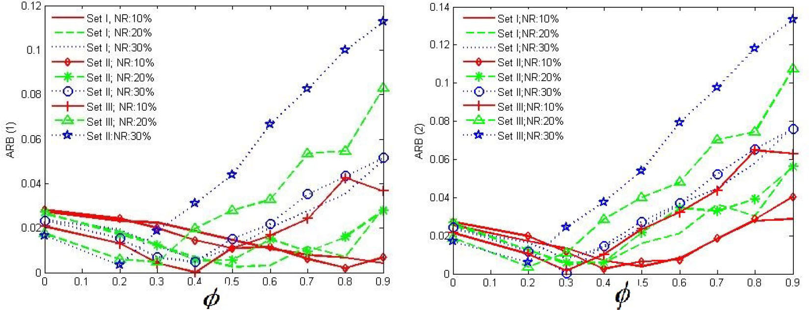
Figures 1 and 2 shows the Absolute relative bias (ARB) and the Percent relative efficiency (PRE) respectively, obtained in the simulation study for several values of $n, m$ and $u$ (termed as sets) and different choices of non-response (NR) rates in AQI population.

Some noteworthy findings from Figs 1 and 2 are as follows:

10. 1.
It is observed that in general, newly tuned jackknife successive estimators in presence of non-response have a small bias and all are within a reasonable range. As far as PRE is concerned the tuned jackknife estimator $\hat{T}^{\textit{NR}}$ is better than $\hat{T}_{s}^{\textit{NR}}$ .
2.
The result confirm the good behaviour in terms of PRE of the newly tuned jackknife successive estimator $\hat{T}^{\textit{NR}}$ (Info U) as compared to $\hat{T}_{s}^{\textit{NR}}$ (Info s) for all sample sizes considered at two occasions and for all non-response rates considered.
3.
It is further observed that for fixed set and fixed non-response rate, as $\phi$ increases the bias of the estimators decreases. However, PRE first decreases and afterwards increases again then finally decreases as $\phi$ increases.
4.
Lower value of $\phi$ indicates more weight is on the estimator for matched portion of the sample and as it is obtained from the units who responded on first occasion. This may be the reason of decrease in bias for increasing $\phi$ .
5.
For fixed $\phi$ and for fixed $n, m$ and $u$ as the non-response rate increases PRE(1) also increase.
6.
From Table 3, it is observed that the optimum value of $\phi_{1}$ and $\phi_{2}$ exists for the estimators $\hat{T}^{\textit{NR}}$ and $\hat{T}_{s}^{\textit{NR}}$ respectively for all sets considered. Further it is vindicated that $\hat{V}(\hat{T}^{\textit{NR}})_{\text{opt.}}$ $<$ $\hat{V}(\hat{T}_{s}^{\textit{NR}})_{\text{opt.}}$ for all sets and all considered non-response rates. This shows that $\hat{T}^{\textit{NR}}$ is better than $\hat{T}_{s}^{\textit{NR}}$ at their respective optimum condition.
7.
From simulation results in Table 4, it is observed that $E_{i}>100∼{}\forall i=1,2$ and $3,$ this shows that the complete response case is always better than non-response cases.
8.
As non-response increases, the value of $E_{i}∼{}\forall i=1,2$ and 3 also increases for fixed $\alpha$ .
9.
In general, it is observed that $E_{1}>E_{3}>E_{2},$ this shows that when non-response is either at both occasions or only at current occasion, then those cases are not better than, the case when non-response is only at first (previous) occasion. This may be due to retaintion of matched sample from the responding units only at first occasion.
10.
For fixed non-response and fixed set as $\alpha$ increases the value of $E_{1}$ and $E_{3}$ increases but $E_{2}$ is almost stable.

8. Concluding remarks

The new concept of tuned jackknife technique is feasible to be applied in successive sampling and is proved to be an useful tool to deal with non-response occuring on successive occasions. The performance of estimator under Info U is better than that under Info s which is in accordance with the theory that as the information on auxiliary variable increases the performance of estimator enhances. Tuned estimators are computer friendly too, which is an added benifit in today’s scenario of digital revolution. Therefore, the methodology proposed may be recommended as useful alternative with a variety of desirable properties to be used by practitioners in this field.

Footnotes

Acknowledgments

Author is thankful to the reviewer for deeply reading the paper and providing constructive suggestions that lead to improvement over the earlier version of the paper. The author is also thankful to SERB, New Delhi, India for providing financial assistance to carry out the present work and sincerely acknowledge the free access to data at www.aqi.in and https://app.cpcbccr.com/AQI_India.

References

Artes

Rueda

, & Arcos

(1998). Successive sampling using a product estimate. Applied Sciences and the Enviornment, Computational Mechanics Publications, 23, 85-90.

Deville

J. C.

, & Särndal

C. E.

(1992). Calibration estimators in survey sampling. J Amer Statist Assoc, 87, 376-382.

Eckler

A. R.

(1955). Rotation sampling. Ann Math Statist, 26(4), 664-685.

Jessen

R. J.

(1942). Statistical investigation of a sample survey for obtaining farm facts. Iowa Agri Exp Stat Res Bull, 304, 1-104.

Lundstrom

, & Särndal

C. E.

(1999). Calibration as standard method for treatment of non-response. Journal of official Statistics, 15, 305-327.

Narain

R. D.

(1953). On the recurrence formula in sampling on successive occasions. J Indi Soci Agri Statis, 5, 96-99.

Okafor

F. C.

(1992). The theory and application of sampling over two occasions for the estimation of current population ratio. Statistica, 1, 137-147.

Patterson

H. D.

(1950). Sampling on successive occasions with partial replacement of units. J Royal Stat Soci, 12, 241-255.

Priyanka

, & Mittal

(2015). A class of estimation for population median in two occasion rotation sampling. HJMS, 44(1), 189-202.

10.

Priyanka

, & Mittal

(2016). Searching effective rotation patterns for population median using exponential type estimators in two occasion rotation sampling. Communications in Statistics-Theory and Methods, 45(18), 5443-5460.

11.

Priyanka

, & Mittal

(2017). New approach using exponential type estimator with cost modelling for population mean on successive waves. Statistics in Transition-new Series, 18(4), 569-587.

12.

Priyanka

Kumar

, & Trisandhya

(2019). Calibration estimators for quantitative sensitive mean estimation under successive sampling. Comm in Stat-Theory and Meth, doi: 10.1080/03610926.2019.1649430.

13.

Rao

J. N. K.

, & Graham

J. E.

(1964). Rotation design for sampling on repeated occasions. Journal of American Statistical Association, 59, 492-509.

14.

Rubin

D. B.

(1976). Inference and missing data. Biometrika, 63, 581-592.

15.

Rueda

Martínez

Arcos

, & Muñoz

J. F.

(2009). Mean estimation under successive sampling with calibration estimators. Comm Stat-Theo and Meth, 38, 808-827.

16.

Sen

A. R.

Seller

, & Smith

D. N.

(1973). The use of ratio estimate in successive sampling. Biometrica, 31, 673-683.

17.

Scott

A. J.

, & Smith

T. M. F.

(1974). Analysis of repeated surveys using time series methods. Journal of the American Statistical Association, 69, 674-678.

18.

Singh

G. N.

, & Priyanka

(2006). On the use of chain-type ratio to difference estimator in successive sampling. International Journal of Applied Mathematics and Statistics, 5(SO6), 41-49.

19.

Singh

G. N.

, & Priyanka

(2010). Estimation of population mean at current occasion in presence of several varying auxiliary variates in two occasion successive sampling. Statistics in Transition-new Series, 11(1), 105-126.

20.

Singh

Sedory

S. A.

Rueda

M. del M.

Arcos

, & Arnab

(2016). A new concept for tuning design weights in survey sampling. Elsevier Publication.

21.

Tikkiwal

B. D.

(1953). Optimum allocation in successive sampling. J Indian Soc Agri Stat, 5, 100-102.

22.

Tikkiwal

B. D.

(1964). A note on two stage sampling on successive occasions. Sankhya, 26(A), 97-100.

Tuning design weights to deal with non-response in successive sampling

Abstract

Keywords

1. Introduction

2. Notations and sampling design

Table 1 Response set and observed values on two occasions

3.1 Tuned jackknife estimator based on fresh sample

5.1 Case-I: When there is non-response only at first (previous) occasion

Table 2 Description of natural population

Footnotes

Acknowledgments

References

Table 1
Response set and observed values on two occasions

Table 2
Description of natural population