Simultaneous prediction of functionally dependent random variables by maximum likelihood estimation

Abstract

The paper presents a fundamental parametric approach to simultaneous forecasting of a vector of functionally dependent random variables. The motivation behind the proposed method is the following: each random variable at interest is forecasted by its own model and then adjusted in accordance with the functional link. The method incorporates the assumption that models’ errors are independent or weekly dependent. Proposed adjustment is explicit and extremely easy-to-use. Not only does it allow adjusting point forecasts, but also it is possible to adjust the expected variance of errors, that is useful for computation of confidence intervals. Conducted thorough simulation and empirical testing confirms, that proposed method allows to achieve a steady decrease in the mean-squared forecast error for each of predicted variables.

Keywords

Simultaneous prediction time series economic indicators seemingly unrelated regressions maximum likelihood estimation linearly dependent random variables

1. Introduction

Very often when modeling some economic entity we encounter a problem of simultaneous time series prediction. In the majority of cases these time series are somehow interconnected as they describe a single object, e.g. a firm, a region, an industry, a country etc. However, many researchers still predict each of the considered economic indicators according to the model specially constructed for it, i.e. separately from the others. Thus, the predicted indicators often appear to be incoherent with each other as above-mentioned interconnections are omitted. If modeled time series are functionally dependent, one can try to tackle this problem with well-known simultaneous equation model (SEM) when all endogenous variables in the structural form are modeled via exogenous ones (reduced form). For example, when predicting indices of the Gross Domestic Product (GDP), the GDP deflator and GDP in constant prices one may use a trivial functional relation, more specifically the GDP index is equal to the product of the GDP deflator index and the real GDP index. This approach preserves the functional link but significantly lacks flexibility and suffers from excessive number of parameters, that dramatically decreases the accuracy of constructed models, see for example Turlach et al. (2005), Yuan and Lin (2006), Yuan et al. (2007) and Gura et al. (2020). Another popular approach to modeling interconnected random variables is seemingly unrelated regressions (SUR), originally proposed by Zellner (1962) and later elaborated by Breiman and Friedman (1997). This method considers regression with multiple responses, i.e. modeling a vector of the target variables. Such models consist of a system of regression equations with the assumption of some degree of correlation between the error terms. A number of papers have been devoted to nonparametric models with two target variables (biresponse models) estimated using smoothing splines, see for example Welsh et al. (2002), Lestari et al. (2010) and Chen and Wang (2011), as well as using the polynomial approximation, see Chamidah et al. (2012). The purpose of such models with multiple responses is to obtain more accurate predictions, since we add information about the interdependence between the errors of predicted variables. This interdependence is usually represented in the form of the variance-covariance matrix of errors, whose inverse is used to weigh observed residuals in calculating the estimates of true model parameters by analogy with the generalized least-squares method. The maximum effect in this case is achieved if there is a sufficiently strong correlation between the errors of modeled processes, which is clearly shown in the works of Ruchstuhl et al. (2000), Guo (2002) and Guo et al. (2011). The downside of SUR is that there is no clear way to compute the variance-covariance matrix of error terms and the majority of papers, devoted to multiple responses topic, are focused on that, see for example Rothman et al. (2008), Rothman et al. (2010), Lee and Liu (2012), Nyangarika et al. (2018) and Nyangarika et al. (2019). Besides that, these models do not fully bring considered random variables into accordance with stated functional link, but rather only decrease the variance of parameters’ estimates. Typically, regression models with multiple responses are widely used in the analysis of categorical or panel data in the field of medicine and sociology, see Wang et al. (2000), Welsh and Yee (2006), Antoniadis and Sapatinas (2007) and Chen and Wang (2011). However, in the field of economics, approaches that share similar idea can produce models of higher quality. This statement is reasoned by the ubiquitous presence of functional dependence among economic indicators of an object of interest. Therefore, in this paper we focus on the general framework of incorporating known functional dependence into the system of equations, which was proposed by Moiseev and Volodin (2019). We expresses an idea that it is possible to improve the accuracy of predictions of functionally dependent indicators by taking into account the dependencies between them. Since almost all functional links between economic indicators are linear (balance sheet, profit and loss account, cash flow statement, system of national accounts, etc.) or can be trivially linearized, we aim at deriving an explicit analytical form for these adjustments for the linear case. It is also worth noting, that this framework of adjustments, besides increasing the forecast accuracy and bringing modeled variables into accordance with their functional link, also does not impose any constraints on the type of constructed models, that tremendously expands its sphere of application.

The paper has the following structure. In Section 2 we propose a method of adjustments, accounting for linear dependencies between modeled indicators when they are simultaneously predicted by models of any nature. Section 3 is devoted to simulation and empirical investigation of proposed method in order to demonstrate its efficiency. Section 4 summarizes the obtained results, highlights the key characteristics of the proposed method and discusses directions for further research.

2. The method

Let $\{y_{t},\mathbf{X}_{t}:t=1,\ldots,n\}$ be a real-valued sample where $y_{t}$ is a target variable and $\mathbf{X}_{t}=(1,x_{1t},x_{2t},\ldots)$ is a countable dataset of possible explanatory variables. Then one can come up with a model of any nature for $y_{t}$ :

$\displaystyle y_{t}=\phi(\mathbf{X}_{t},\theta)+\varepsilon_{t},$ (1)

where $\theta$ is a parameter column-vector.

The only requirement for such model is that it returns an unbiased forecast and mean squared forecast error, which is subject to normal distribution. Further, suppose that there is a set of target variables $y^{(1)}_{t},y^{(2)}_{t},\ldots,y^{(K)}_{t}$ , each of which is modeled using the data set $\mathbf{X}_{t}^{(1)},\mathbf{X}_{t}^{(2)},\ldots,\mathbf{X}_{t}^{(K)}$ respectively. Besides that, there is a known functional form that binds all considered target variables together:

$\displaystyle y^{(i)}_{t}=f_{i}\left(y^{(1)}_{t},\ldots,y^{(i-1)}_{t},y^{(i+1)% }_{t},\ldots,y^{(K)}_{t}\right),$ (2)

where $f_{i}$ denotes a function, which expresses $y^{(i)}_{t}$ in terms of other explanatory variables under consideration.

Hence we make the following assumption to ensure the reliability of further derivations.

Assumption 1. Absence of correlation between errors of target variables under consideration, i.e. $\text{cov}\left({\varepsilon}^{(i)}_{t};{\varepsilon}^{(j)}_{t}\right)=0,% \forall i\neq j$ . Note that this condition is usually satisfied when modeling vectors with a sufficiently large number of indicators and their volatility is comparable in magnitude.

Then according to Moiseev and Volodin (2019) it is possible to correct obtained predictions, taking into account their probability density functions $\Psi_{i}\left(y^{(i)}_{n+1}\right)$ and a known functional relationship between the target variables. This procedure is proposed to be carried out using the Maximum Likelihood Method (MLM), which maximizes the likelihood function, which is the joint probability density of a set of analyzed random variables. In the case of the functionally dependent target variables mentioned above, the joint probability density can be represented as follows in terms of the function $f_{1}$ :

$\displaystyle LH={\Psi}_{1}\left(f_{1}\left[y^{(2)}_{n+1},y^{(3)}_{n+1},\ldots% ,y^{(K)}_{n+1}\right]\right)\cdot{\Psi}_{2}(y^{(2)}_{n+1})\ldots{\Psi}_{K}(y^{% (K)}_{n+1}).$ (3)

Thus, the procedure of adjusting the forecasts is reduced to finding such values of predicted random variables that would maximize expression Eq. (3). In order to reduce computational complexity of calculating the optimal parameters when maximizing the likelihood function Eq. (3), we resort to the maximization procedure for its log-likelihood function.

$\displaystyle\log-LH=\ln\left\{{\Psi}_{1}\left(f_{1}[y^{(2)}_{n+1},y^{(3)}_{n+% 1},\ldots,y^{(K)}_{n+1}]\right)\right\}+\ln\left\{{\Psi}_{2}(y^{(2)}_{n+1})% \right\}+\ldots+\ln\left\{{\Psi}_{K}(y^{(K)}_{n+1})\right\}.$ (4)

Therefore, by applying the correction by maximizing the log-likelihood function Eq. (4) we adjust obtained forecasts in order to bring them into coherence by initially stated functional link. In addition to proposed adjustments to traditional predictions, it is also possible to obtain the adjusted probability density function for all target variables under consideration. This procedure is proposed to be carried out by calculating the marginal distribution for the analyzed target variable, which takes into account probability distributions of the remaining target variables and the functional relationship between them. Thus, according to this method, corrected probability density function is calculated as shown below:

$\displaystyle\text{pdf}\left(y^{(i)}_{n+1}\right)=\frac{\Omega\left(y^{(i)}_{n% +1}\right)}{\int^{\infty}_{-\infty}{\Omega\left(y^{(i)}_{n+1}\right){\rm d}y^{% (i)}_{n+1}}},$ (5)

where the normalizing constant in the denominator is an integral of the likelihood function over all target variables under consideration, and $\Omega(y^{(i)}_{n+1})$ is computed as follows:

$\displaystyle\Omega\left(y^{(i)}_{n+1}\right)=\int^{\infty}_{-\infty}\ldots% \int^{\infty}_{-\infty}{\Psi}_{1}\left(y^{(2)}_{n+1}\right)\ldots\Psi_{i-1}% \left(f_{i-1}\left[y^{(1)}_{n+1},\ldots y^{(i-1)}_{n+1},y^{(i+1)}_{n+1},\ldots% ,y^{(K)}_{n+1}\right]\right)\cdot{\Psi}_{i}\left(y^{(i)}_{n+1}\right)\ldots{% \Psi}_{K}\left(y^{(K)}_{n+1}\right)dy^{(1)}_{n+1}\ldots{\rm d}y^{(i-1)}_{n+1}{% \rm d}y^{(i+1)}_{n+1},\ldots,{\rm d}y^{(K)}_{n+1}.$ (6)

Hence, for the sake of simplicity we slightly change notation as follows: $y^{(i)}_{n+1}=y_{i}$ .

In this paper we will focus on a particular case where modeled target variables represent a simple linear equation $y_{K}=\sum_{i=1}^{K-1}y_{i}$ , the error term for each model $\varepsilon_{i}\sim N(0,\sigma_{i})$ and assumption 1 holds. Then adjusted probability density function Eq. (5) for $y_{1}$ can be presented as below:

$\displaystyle\text{pdf}(y_{1})=\frac{\displaystyle\idotsint_{\mathbb{R}^{K-2}}% \frac{1}{\sqrt{2\pi}^{K}\prod^{K-1}_{i=1}\sigma_{i}}\prod^{K-1}_{i=1}e^{-\frac% {(y_{i}-\mu_{i})^{2}}{2\sigma^{2}_{1}}}e^{-\frac{\left(\sum^{K-1}_{i=1}y_{i}-% \mu_{K}\right)^{2}}{2\sigma^{2}_{K}}}{\rm d}y_{2}\ldots{\rm d}y_{K-1}}{% \displaystyle\idotsint_{\mathbb{R}^{K-1}}\frac{1}{\sqrt{2\pi}^{K}\prod^{K}_{i=% 1}\sigma_{i}}\prod^{K}_{i=1}e^{-\frac{(y_{i}-\mu_{i})^{2}}{2\sigma^{2}_{1}}}e^% {-\frac{\left(\sum^{K-1}_{i=1}y_{i}-\mu_{K}\right)^{2}}{2\sigma^{2}_{K}}}{\rm d% }y_{1}\ldots{\rm d}y_{K-1}},$ (7)

that can be easily extended to any $y_{i}$ . Here we want to show that, in case all above-mentioned assumptions hold, adjusted probability density for each target variable is subject to normal distribution and has a smaller variance, than the original pdf, that implies higher forecast accuracy, see Theorem 1 in Appendix.

Thus, we propose an easy-to-make adjustment for simultaneous prediction of linearly dependent random variables that does not impose any requirements on the model’s nature, for instance one target variable can be modeled by ARIMA model, another – by neural network and so on. The only important thing is that these models are supposed to return unbiased point forecast and its variance. Such adjustment helps increase the accuracy of constructed models by adding information about the functional link of predicted processes.

3. Empirical and simulation testing of proposed method

In order to test efficiency of the method proposed in this paper, we carry out simulation and empirical experiments. First, we check how well these adjustments work for generated data. Let us consider a simple case, when a set of target variables $y_{1},y_{2},\ldots,y_{K}$ is generated by first order autoregression model, namely:

$\displaystyle y_{it}={\beta}_{i0}+{\beta}_{i1}y_{i(t-1)}+{\varepsilon}_{it}% \forall i\neq K,$ $\displaystyle y_{Kt}=\sum_{i=1}^{K-1}y_{it}.$ (8)

Error terms $\varepsilon_{it}$ are generated from normal distribution with zero mean and $\sigma_{i}=0.5$ . Experiment designs are presented in Table 1.

Table 1

Simulation experiment designs

No.	$K$	True parameters
1	3	$\beta_{i0}=2$ , $\beta_{11}=0.3$ , $\beta_{21}=0.5$
2	5	$\beta_{i0}=2$ , $\beta_{11}=0.2$ , $\beta_{21}=0.4$ , $\beta_{31}=0.6$ , $\beta_{41}=0.8$

Table 2

Simulation experiment results, MSRFE for design 1

$n$	1	2	3	adj 1	adj 2	adj 3	$1+2$
10	0.3192	0.3622	0.6908	0.3134	0.3509	0.6525	0.6876
20	0.3108	0.3709	0.7035	0.3081	0.3571	0.6645	0.6967
40	0.3046	0.3549	0.6546	0.3025	0.3451	0.6328	0.6567
80	0.2991	0.3491	0.6599	0.3003	0.3426	0.6474	0.6571
120	0.2909	0.3399	0.6335	0.2925	0.3346	0.6264	0.6337

Generated time series were then forecasted one-step-ahead by auto.arima function from R environment, which selects the form of SARIMA class model by minimizing Akaike information criterion (AIC). To provide a comprehensive simulation experiment, all designs were tested on windows of different lengths $n$ and compared by the mean-squared realized forecast error. To compute the results for each window size we used 10,000 simulations. Therefore, this experiment can be considered as a basis for making sound conclusions about the efficiency of proposed adjustments. Of course such experiment designs will result in a violation of above-mentioned assumptions of independence of the error terms for different models (due to using information from all $y_{i}$ , $i\neq K$ to model $y_{K}$ ) and their normality (due to relatively short windows). But despite this fact, as will be shown further, proposed adjustments on average increase the forecast accuracy for modeled indicators.

Table 2 shows the mean square realized forecast error for models for design 1, numbered respectively. The last column labeled “ $1+2$ ” denotes the model, forecasting $y_{3}$ by simply summing up the predictions of initial models for $y_{1}$ and $y_{2}$ .

As it can be seen from Table 2, proposed method of correcting predicted target variables exceeds initial models in accuracy for almost any data frame under consideration (highlighted in bold). The only exception is the mean-squared realized error for $y_{1}$ for $n=80$ and $n=120$ . But even for these cases proposed adjustment is only slightly losing to initial model, see Fig. 1.

Table 3 displays the mean square realized forecast error for models for design 2, numbered respectively.

Table 3

Simulation experiment results, MSRFE for design 2

$n$	1	2	3	4	5	adj 1	adj 2	adj 3	adj 4	adj 5
10	0.2933	0.3417	0.3936	0.4579	1.5379	0.2942	0.3387	0.3837	0.4412	1.3781
20	0.2832	0.3434	0.3949	0.4711	1.5665	0.2856	0.3414	0.3872	0.4584	1.4069
40	0.2754	0.3279	0.3972	0.4591	1.5408	0.2806	0.3289	0.3916	0.4475	1.4191
80	0.2751	0.3206	0.3834	0.4536	1.4368	0.2778	0.3219	0.3794	0.4405	1.3837
120	0.2699	0.3055	0.3689	0.4521	1.4222	0.2734	0.3076	0.3659	0.4405	1.3749

Figure 1.

Simulation experiment results, MSRFE for design 1.

Analyzing results from Table 3 we observe almost the same pattern as from Table 2. Proposed method slightly underperforms for initial models with relatively low MSRFE ( $y_{1}$ and $y_{2}$ ), but for that significantly outperforms models with relatively large MSRFE ( $y_{3}\ldots y_{5}$ ), that is also displayed in Fig. 2. Low MSRFE is usually observed for target variables that are generated with smaller coefficient $\beta$ , since there is less bias in estimating true parameters.

Figure 2.

Simulation experiment results, MSRFE for design 2.

It is also worth noticing, that for all target variables and both methods under consideration, the accuracy of the prediction increases with the extension of the window, the difference between adjusted forecasts and initial ones also shrinks. However, when analyzing time series of economic processes, one very often has to work under conditions of the scarcity of statistical data. It is well known that a too long data frame yields just as inaccurate forecasts as does a too short one. Therefore, when analyzing economic processes, application of proposed adjustments allows a significant reduction of the forecast error.

Next, let us proceed to the empirical testing of the method, which takes into account the linear dependence of the modeled target variables. Consider the simplest three-factor macroeconomic equation

$\displaystyle I_{\text{RGDP}}\times I_{\text{Deflator}}=I_{\text{GDP}},$ (9)

which can be easily linearized as follows:

$\displaystyle\ln(I_{\text{RGDP}})+\ln(I_{\text{Deflator}})=\ln(I_{\text{GDP}}).$ (10)

We took the quarterly statistics for the USA for these indicators, starting from Q1.1947 to Q2.2019. Thus, the set of statistical data for carrying out the empirical experiment constitutes 290 observations. Table 4 shows the mean-squared realized forecast error of models for each variable in Eq. (10), constructed by one-step-ahead rolling window procedure, using auto.arima function from R environment, and their adjustments according to proposed method.

Table 4

Empirical experiment results, MSRFE for RGDP, Deflator and GDP

$n$	RGDP	adj RGDP	Deflator	adj Deflator	GDP	adj GDP
10	0.7082	0.6525	0.0912	0.0901	0.6845	0.6845
20	0.7854	0.6399	0.0824	0.0801	0.6301	0.6742
30	0.6387	0.5746	0.0680	0.0677	0.6103	0.6076
40	0.6514	0.5959	0.0759	0.0745	0.6503	0.6277
50	0.6072	0.5651	0.0708	0.0719	0.6253	0.5934
60	0.6013	0.5670	0.0708	0.0705	0.6192	0.6077
70	0.5973	0.5709	0.0754	0.0747	0.6268	0.6126
80	0.6155	0.5658	0.0753	0.0740	0.6204	0.6191
90	0.6157	0.5900	0.0763	0.0746	0.6514	0.6437
100	0.5551	0.5441	0.0687	0.0687	0.6225	0.5928

As it can be seen from Table 4 almost for all $n$ proposed adjustments display higher accuracy for three considered macroeconomic indicators. Figure 3 illustrates the positive effect of such adjustments, which is especially clear for $\ln(I_{\text{RGDP}})$ and $\ln(I_{\text{RGDP}})$ due to their relatively large magnitude of MSRFE.

Figure 3.

Empirical experiment results, MSRFE for RGDP, Deflator and GDP.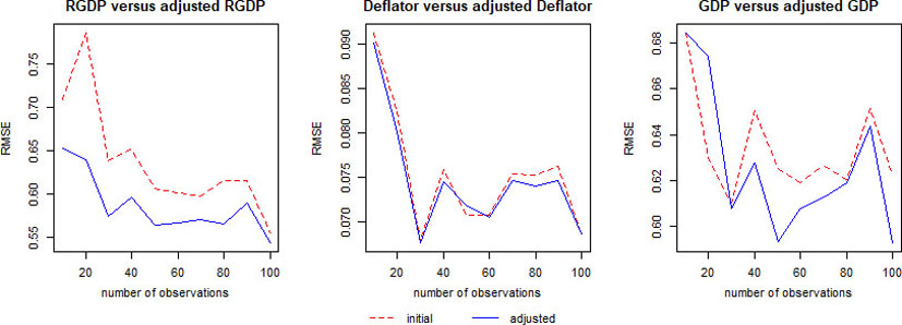

Thus, we can conclude, that proposed method results in a significant improvement of simultaneous forecasts of linearly dependent random variables, what is especially distinct under conditions of a short window. Though assumptions, imposed in Section 2, very rarely hold in practice, nevertheless the method performs well even if they are not fully met. The reason for such an improvement is that by incorporating known functional link we reduce the uncertainty concerning model specification and parameters estimates. Moreover, in distinct from SUR, proposed method does not impose any requirements on model’s nature. It is obvious, that positive effect from these adjustments is gradually canceled out with increasing number of observations. However, despite the fact that for a long data frame, the difference between the analyzed approaches is minimal, this method is still relevant, because when modeling economic processes the sufficiency of statistical data is extremely rare.

4. Conclusion

The paper presents a method of increasing the forecast accuracy when simultaneously predicting a set of linearly connected random variables. In the first step each target variable is predicted by its own model (without any requirements on model’s nature); afterwards obtained predictions are adjusted to satisfy their linear connection, using explicit and easy-to-use formula. Along with correcting predictions, we also explicitly correct the expected forecast variance, that allows one to easily compute the interval forecast. The simulation and empirical experiments show, on fairly trivial examples, practical benefits of proposed method. When making such corrections, obtained forecasts become coherent with each other, that positively affects their quality. In general, developed methods result in a significant improvement in the quality of forecasts in comparison with the regression equations that model each target variable separately. This positive effect is achieved due to the use of information about the form of the functional or dependence between the forecasted target variables. Since we can functionally bind the majority of economic indicators, proposed method can be considered relevant for complex simultaneous forecasting of economic processes.

Footnotes

Acknowledgments

This research was performed in the framework of the state task in the field of scientific activity of the Ministry of Science and Higher Education of the Russian Federation, project “Development of the methodology and a software platform for the construction of digital twins, intellectual analysis and forecast of complex economic systems”, grant no. FSSW-2020-0008.

Appendix

Theorem 1. Let $\mathbf{y}_{i}=(y_{1},y_{2},\ldots,y_{K})$ , be a set of predicted values, which satisfy the following functional link $y_{K}=\sum_{i=1}^{K-1}y_{i}$ , assumption 1 holds and respective error terms are subject to normal distribution with zero mean and constant variance. Then pdf for every modeled target variable Eq. (7) is also gaussian with variance $\hat{\sigma}^{2}_{i}$ and mean $\hat{\mu}_{i}$ , explicitly computed as below:

(11) $\displaystyle\hat{\sigma}^{2}_{1}=\frac{\sigma^{2}_{1}\sum_{i=2}^{K}\sigma^{2}% _{i}}{\sum_{i=1}^{K}\sigma^{2}_{i}}∼{}(\mbox{can be extended to any∼{}}\hat{% \sigma}_{i}),$

where $\sigma^{2}_{i}$ is variance of initially forecasted $i$ -th target variable $y_{i}$ ,

(12) $\displaystyle\hat{\mu}_{1}=\frac{\mu_{1}\sum_{i=2}^{K}\sigma^{2}_{i}+\sigma^{2% }_{1}(\mu_{K}-\sum_{i=2}^{K-1}\mu_{i})}{\sum_{i=1}^{K}\sigma^{2}_{i}}∼{}(\mbox% {can be extended to any∼{}}\hat{\mu}_{i},\mbox{except for∼{}}\hat{\mu}_{K}),$

where $\mu_{i}$ is an initially obtained mean for the forecast of the $i$ -th target variable $y_{i}$ ,

(13) $\displaystyle\hat{\mu}_{K}=\frac{\mu_{K}\sum_{i=1}^{K-1}\sigma^{2}_{i}+\sigma^% {2}_{K}\sum_{i=1}^{K-1}\mu_{i}}{\sum_{i=1}^{K}\sigma^{2}_{i}}.$

Besides that $\hat{\sigma}^{2}_{i}<\sigma^{2}_{i}∼{}\forall i$ .

Proof In order to prove it we integrate the equation Eq. (7) and get

(14) $\displaystyle\text{pdf}(y_{1})=\sqrt{\frac{\sum_{i=1}^{K}\sigma^{2}_{i}}{2\pi% \sigma^{2}_{1}\sum_{i=2}^{K}\sigma^{2}_{i}}}e^{-\frac{1}{2}\frac{\sum_{i=1}^{K% }\sigma^{2}_{i}}{\sigma^{2}_{1}\sum_{i=2}^{K}\sigma^{2}_{i}}\left(y_{1}-\frac{% \mu_{1}\sum_{i=2}^{K}\sigma^{2}_{i}+\sigma^{2}_{1}\left(\mu_{K}-\sum_{i=2}^{K-% 1}\mu_{i}\right)}{\sum_{i=1}^{K}\sigma^{2}_{i}}\right)^{2}}.$

By definition of gaussian distribution, from Eq. (14) it is clear, that the adjusted variance and mean are explicitly expressed like in Eqs (11)–(13). Given the derived analytical form for $\hat{\sigma}^{2}_{1}$ it is easy to show that $\hat{\sigma}^{2}_{1}<\sigma_{1}^{2}\forall\sigma_{i}^{2}>0$ and $\lim_{\sigma_{i}^{2}\rightarrow\infty}\hat{\sigma}^{2}_{1}=\sigma_{1}^{2}\forall i$ .

Detailed proof can be provided upon request.

References

Antoniadis

, & Spatinas

(2007). Estimation and inference in functional mixed-effects models. Computational Statistics and Data Analysis, 51(10), 4793-4813.

Breiman

, & Friedman

J. H.

(1997). Predicting multivariate responses in multiple linear regression. Journal of the Royal Statistical Society Series B, 59, 3-54.

Chamidah

Budiantara

I. N.

Sunaryo

, & Zain

(2012). Designing of child growth chart based on multiresponse local polynomial modeling. Journal of Mathematics and Statistics, 8(3), 242-247.

Chen

, & Wang

(2011). A penalized spline approach to functional mixed effects model analysis. Biometrics, 67(3), 861-870.

Guo

Levina

Michailidis

, & Zhu

(2011). Joint estimation of multiple graphical models. Biometrika, 98, 1-15.

Guo

(2002). Functional mixed effects models. Biometrics, 58(1), 121-128.

Gura

Mikhaylov

Glushkov

Zaikov

, & Shaikh

Z. A.

(2020). Model for estimating power dissipation along the interconnect length in single on-chip topology. Evolutionary Intelligence.

Lee

, & Liu

(2012). Simultaneous multiple response regression and inverse covariance matrix estimation via penalized gaussian maximum likelihood. Journal of Multivariate Analysis, 111, 241-257.

Lestari

Budiantara

I. N.

Sunaryo

, & Mashuri

(2010). Spline estimator in multi-response non-parametric regression model with unequal correlation of errors. Journal of Mathematics and Statistics, 6(3), 327-332.

10.

Moiseev

N. A.

, & Volodin

(2019). Increasing the accuracy of macroeconomic time series forecast by incorporating functional and correlational dependencies between them. Applied Econometrics, 53(1), 119-137.

11.

Nyangarika

Mikhaylov

, & Tang

B. J.

(2018). Correlation of oil prices and gross domestic product in oil producing countries. International Journal of Energy Economics and Policy, 8(5), 42-48.

12.

Nyangarika

Mikhaylov

, & Richter

(2019). Oil price factors: Forecasting on the base of modified auto-regressive integrated moving average model. International Journal of Energy Economics and Policy, 9(1), 149-160.

13.

Rothman

A. J.

Bickel

P. J.

Levina

, & Zhu

(2008). Sparse permutation invariant covariance estimation. Electronic Journal of Statistics, 2, 494-515.

14.

Rothman

A. J.

Levina

, & Zhu

(2010). Sparse multiple regression with covariance estimation. Journal of Computational and Graphical Statistics, 19, 947-962.

15.

Ruchstuhl

Welsh

A. H.

, & Carroll

R. J.

(2000). Nonparametric function estimation of the relationship between two repeatedly measured variables. Statistica Sinica, 10(1), 51-71.

16.

Turlach

B. A.

Venables

W. N.

, & Wright

S. J.

(2005). Simultaneous variable selection. Technometrics, 47, 349-363.

17.

Wang

Guo

, & Brown

M. B.

(2000). Spline smoothing for bivariate data with application to association between hormones. Statistica Sinica, 10(1), 377-397.

18.

Welsh

A. H.

Lin

, & Carroll

R. J.

(2002). Marginal longitudinal nonparametric regression: Locality and efficiency of spline and kernel methods. Journal of American Statistical Association, 97(458), 482-494.

19.

Welsh

A. H.

, & Yee

T. W.

(2006). Local regression for vector responses. Journal of Statistical Planning and Inference, 136(9), 3007-3031.

20.

Yuan

, & Lin

(2006). Model selection and estimation in regression with grouped variables. Journal of the Royal Statistical Society Series B, 68, 49-67.

21.

Yuan

Ekici

, & Monteiro

(2007). Dimension reduction and coefficient estimation in multivariate linear regression. Journal of the Royal Statistical Society Series B, 69, 329-346.

22.

Zellner

(1962). An efficient method of estimating seemingly unrelated regression equations and tests for aggregation bias. Journal of the American Statistical Association, 57(298), 348-368.

23.

Zhang

H. H.

Liu

, & Zhu

(2008). Variable selection for the multicategory svm via adaptive sup-norm regularization. Electronic Journal of Statistics, 2, 149-167.