Beauty or money? Statistical analysis

Abstract

There are many studies investigating relationship between paintings’ meta information (author, age, etc.) and their prices, however, there is limited research on how people’s aesthetic perception of paintings is related to their prices. To bridge this gap, we designed a website (pollart1000.com) collecting survey responses on people’s opinions regarding aesthetic values of paintings; survey and data were complemented with price information. Comprehensive statistical analysis of that data is presented, including scoring of the best and worst works, correlations between variables, typology of respondents, and more. The results quantify relationships between aesthetic values and art prices. Particularly, we showed that aesthetic preference is inclined to figurative and innovational rather than to abstract art and that relations between price and aesthetic values are rather weak except of special cases.

Keywords

Art price models painting aesthetic value metrics of aesthetics statistical analysis of art

1. Introduction

The recent events on a top of the “monetary ladder” in art, where closest neighbors now are pieces by such different artists as Leonardo da Vinci ($452M) and Willem de Kooning ($300M), revitalized the question about relationship between aesthetics and economic value in art. What people do pay money for? For “beauty”? For a “big name”? “For investment purposes”? Can one estimate that relation numerically?

Questions like that have been long standing. In a thorough overview of the early history (Marchi, 2009) it is traced back to de Piles (1708), Richardson (1719), and then through different contributions by famous economist Smith, political thinker Bentham, and others, to works by one of the founders of mathematical economics Jevons and initiators of the conference “Aesthetics of Value” in 1870s.

The very first attempt by de Piles in 18th century was to estimate “56 of the best-known painters $\ldots$ for their performance in the four dimensions, composition, design, coloring, and expression” (Marchi, 2009, p. 98). Among the painters were: Romano, who on the 1–10 scale (10 is the best) had received 4 for coloring; Reni, with 1 for composition; Rembrandt with 6 for design; and Titian with 6 for expression. All the scores could be disputed but for that time it was a huge brave leap ahead.

Richardson, who considered the art estimation as a “Science of a Connoisseur”, extended the de Piles’ list to 8 attributes: Composition, coloring, handling, drawing, invention, expression, grace, and greatness. The novelty was in that he estimated not artists, but separate paintings (especially portraits), and that he gave some general characteristics of the works of art, like Advantage or Pleasure, together with eight more specific features. His notion of “Intrinsic Qualities of the thing itself” (Marchi, 2009, p. 100), was really the first concept of “objective quality of art,” strongly defended by Birkhoff (1933) more than two hundred years later.

Qualitatively, important aspects of “pleasure” and market value were considered by Adam Smith, who “pointed to all the causal factors …, but …did not develop a pleasure index, nor did he try to quantify the role of any one of the causal factors” (Marchi, 2009, p.105).

The pioneering works of the 18-th century did not spark a lot of interest among scholars in creating the “pleasure indexes” or similar indicators in measurable form. As late as in 1966, a famous art historian Gombrich treated de Piles’ numerical exercise as “notorious aberration” (Ginsburgh & Weyers, 2009, p. 112). But the relationship between aesthetic and economic values, touched in those works for the first time, were actively discussed, although mainly theoretically, among different researchers, especially philosophers. Complex questions about different values of art (economic, aesthetic, propaganda, theological, moral, therapeutic, prurient, and decorative) were considered in (Lopes, 2011), where the author, after taking into account many different opinions in philosophical literature, concludes that artistic and aesthetic values are actually the same. In (Spaenjers et al., 2015) even more aspects of the art value (especially related to economics) are considered.

Different aesthetic indicators have been the subject of many studies, both theoretical and empirical; a thorough overview can be found in (Markovi & Radonji, 2008). A lot have been said about relations between economic and aesthetic values in theoretical aspects – see many references in (Spaenjers et al., 2015). There were special studies about different relations between elements of art, like “angles” versus “rounds”, and other (Locher, 2012); “art consumers” (like behavior of visitors in museums – see in Mastandrea et al, 2009); titles and prices (Park et al, 2021); and a national identity as a factor (Mastandrea et al., 2019). However, when it comes to quantitative measurement of the relations between economics and aesthetics, the number of studies is surprisingly small.

In (Ginsburg & Weyers, 2009), the authors took de Piles’ estimates of the quality of 56 painters as four independent variables and used them for considering two dependent variables they calculated. The first one was the number of lines about a given painter in the most comprehensive art dictionary (Turner, 1996). The second one was a price estimate for all paintings of a given painter sold on auctions during 1977–1993 (525 transactions). The coefficients of multiple determination of the models by de Pile’s factors (dimensions, composition, design, coloring, and expression) were relatively high, over 30%.

In a similar study (Throasby & Zednik, 2014), the experiment was designed in another way. The authors asked visitors of the gallery in Sydney, Australia, to estimate the economic and aesthetic (cultural) values of six different paintings. After 3 days of the experiment, they gathered a comparatively high number of responses in 480 filled questionnaires and conducted regression analysis based on the answers. This study has a few advantages over the work by Ginsburg and Weyers (2009) with only a single person in the study. The people looked at real art objects, not photographs; however, there were a few potential flaws: the visitors of the gallery were not typical population representatives; the number of paintings was too small; Australian aboriginal works played disproportionally high role (2 out of 6). The key limitation was the fact that respondents were given the actual market prices of all works to create their own “economic value.” It inevitably created a bias, not only the anchoring effect, admitted by the authors (respondents’ price estimates were anchored to actual prices known to them), but of another type: if one knows that this is a very expensive painting, she could value it higher in aesthetic terms as well. And this bias was greatly amplified by the fact that paintings were extremely heterogeneous: prices varied from $6k to $2.5M, which is substantial range for such a small sample. It could be the main reason of the high value of the coefficient of multiple determination 66% for the market price. The model had many predictors, but the role of one variable of the aesthetics estimate was the most important.

In another study on art and persuasion, Mastandrea and Crano (2019) aimed to determine whether artworks, being presented as created by famous artists, will be appreciated higher than the same artworks, when they are attributed to non-famous artists. Findings showed that the works attributed to famous artists were more appreciated than the same works attributed to non-famous artists. In particular, participants were willing to pay more to see the artworks in a museum, if those were described as created by famous artists.

However, lack of models with aesthetic variables does not mean a shortage of general models for the art prices. Likely started by Anderson (1974), boosted by the influential work by Baumol (1986) about repeated sales, very carefully modeled on a huge number of paintings by several scholars (Goetzmann et al., 2013; Penasse et al., 2014), it culminated in the very important recent study (Korteweg et al., 2017), based on repeated sales of more than 30,000 pieces of art. These and other studies (for example, Marinelli & Palomba, 2008, about 2,800 pieces; Bocart & Hafner, 2012, about 550 pieces; Teti, et al., 2014, about 300 pieces) mainly employed a technique of the so called “hedonic regression” and did not use aesthetic value in their models. Characteristically, the scholars admitted the importance of the aesthetics’ value, and in (Teti et al., 2014) the authors stated that without it, any art price models would be “ephemeral” and “fruitless,” but they had not explored the problem further.

Let us look closer at, possibly, the most comprehensive study of this type (Renneboog & Spaenjers, 2013). The authors used the very reliable source of data – auction sales of 1957–2007, as opposite to galleries and other types of sales where data usually is not available. There were 10,442 various artists lived in different times from Medieval to present. The total number of transactions, including repeated ones, was 1,088,709 (about 60% oils, and the others split almost evenly between drawings and watercolors). It is a huge amount of data which could yield reliable conclusions for such problems as return on investment. What did it say about the aesthetic and art-historical value of the works? Out of around 50 independent variables used in regression, there was just one which could be related to the art-historic value – it occurred to be a binary variable with the value 1 if before sale an artist was included in the last edition of the catalogue (Tansev et al., 1995) and 0 otherwise. Therefore, it relies exclusively on just one source – the knowledge of the painter’s importance, which is strongly dependent on the source used, such as mentions in the art dictionaries and critics’ opinions. In addition, the aesthetics is not clearly presented within those 50 variables. Styles of paintings (impressionism, surrealism, etc.), or genre (landscape, portrait, etc.) have very remote relation to the aesthetics, if any.

The lack of aesthetic variables in modeling could be explained by the fact that aesthetic values are very hard to measure. One cannot collect data from the auction houses and make cumbersome aesthetic measurement for many thousands of paintings by multitudes of people. This problem, possibly, will never be solved in a satisfactory manner. The current proposed study is one of the ways to find an approximate solution.

In light of all discussed and other issues the situation looks quite puzzling. The world art market is huge; for the last 15 years it was fluctuating around $62B per year (with one exception, $40B, in 2009, after the financial crisis). What do people pay that money for? Which of the “values of art” play a decisive role “Rarity”? Beauty? “Cult-following”? If the relationship between the aesthetics and market value is not clearly and numerically understood – the whole area of the “art economics” (Heilbrun & Gray 2009; Amariglio et al., 2009; Spranzi, 2008) looks like a castle built on shifting sands. Art economics should address many very practical questions, like state’s funding of museums, creation of curriculum in colleges, sponsoring artists, etc., but without a clear understanding of relations between “money” and “beauty” it hardly could be done. Finally, what is art if it does not create an aesthetic value? And if it does, but no one pays for it – should such an art be discouraged? If it does not, but still gets the highest price tag, should it be encouraged? How does that fit a societal wellbeing? Should the art be reduced merely to its market value, as all quoted studies tried to model? Should one agree that “In practice, art is actually traded as an investment. This is empirically confirmed by activity from dealers, funds …who store artworks in warehouses, or bank vaults…where obviously the aesthetic return is null” (Bocart & Hafner, 2012, p. 3092), or is there anything else behind it? What do unbelievable prices of the past years mean? Is that just the market’s whim with a hope to sell it even higher soon, or are there other reasons?

All these and related questions motivated us to conduct an experiment to understand better the relations between the aesthetic and economic aspects of art in a more systematic way than it was done before.

On a different vein, the relationship between such different fields as statistics and art is not too often discussed in statistical journals (see Lipovetsky & Mandel, 2007, 2009; Mandel & Lipovetsky, 2007). In that sense the paper feels the gap, because it is not only describing the application, but also proposes some simple methods and models which help to deal with data of the specifical structured nature.

The rest of the paper is organized as follows. Section 2 describes different types of data used in the study, including a created website pollart1000.com and its design. Section 3 contains analysis of the collected data. Finally, Section 4 summarizes the findings.

2. Data and survey design

In this paper only a high-level description of the data and experiment are presented; more details could be found in (Mandel, 2020). A hundred painters were selected based on certain procedure from the list provided in Murray (2004). They all are outstanding painters who entered an exclusive list of 600 $+$ “significant painters of Western tradition” out of potential hundreds of thousands of painters during last millennia. Each artist has the so-called Murrays’ Index (referred to later as MI), varied from 100 (the best painter; turned out to be Michelangelo) to 1. For each painter 10 works were presented: 5 most expensive and 5 randomly selected, totaling to 1,000 pieces, although much smaller number was actually used in the analysis.

Each painting had an estimated auction price (hammer plus premium) paid at the time of the latest auction for this piece, transformed into values comparable over time, in dollars as of the end of 2015. The most expensive work was Les femmes d’Alger by Pablo Picasso ($179,365,000) and the cheapest – Cavalier on horseback in a field by Giovanni Fattori ($1,059). The difference in about 170,000 times is a good illustration of what art prices are, considering that all those artists were by definition the “significant figures”. In addition, many other parameters were also collected and analyzed in (Mandel, 2020).

Following (Markovi & Radonji, 2008) and our own intuition and understanding, the following list of variables was used to measure aesthetical values, rated from 1 to 7 (1 – I don’t like it at all; 7 – magnificent, I like it a lot): General Aesthetic Impression, Harmony, Relaxation, Hedonic Value, Arousal, and Technical perfection. The presentation was supported by visual four examples for the best and worst scores with comments, helping respondents to understand what they are asked to focus on. Examples are presented in (Mandel, 2020, Annex 2).

Collecting estimates through an online survey was not an easy task. The key challenge was that one cannot expect a person to spend time rating all 1000 pieces in our database. Ideally, if each work could get at least 30 estimates (usually considered as sufficient for making a statistical inference) – but how to ensure for those desired 30,000 estimates to be evenly distributed among all pieces?

2.1 The design of experiment

After logging into her account in pollart1000.com for the first time, a new user is asked to answer some demographic questions. This information is collected once and is not asked again in subsequent ratings by the same user. Then paintings’ evaluation questions are displayed, with the questions at the top and the painting at the middle part of the screen.

The Likert scale was used to express user’s agreement with the questions, with 1 being the minimal agreement and 7 as the complete agreement. Each respondent has to rate all 10 paintings of each artist selected for evaluation. The artists displayed are selected due to the following algorithm:

(1) (1)
The system picks an artist with the minimum number of already obtained evaluations from the list of all artists having less than 300 estimates (30 for each painting); if there are several artists with minimal number of estimates then it selects one randomly. Within the selected artist the system displays the paintings according to their number of evaluations starting with the least evaluated, then second least evaluated, etc.;
(2)
The selected artist is displayed until getting 300 estimations (at least 30 for each of this artist’s ten paintings), then the system returns to step (1);
(3)
If a user has evaluated all 10 paintings of the artist, he/she is offered to evaluate next artist, also with a minimal number of evaluations.

If a respondent discontinues the session at any point, it is saved, and next time she can continue from the point of stoppage. For example, if she dropped the experiment after the third painting of an artist X, the next time she will be offered to evaluate the fourth painting of the artist X.

The first version of the website pollart1000.com was released in July 2016. Collection of data was boosted by the authors via advertising among their friends and via social media. The key characteristics of respondents are given in Table 1 as of 9/07/2017 (data collection was stopped after that date).

Table 1
Demographics of participants at the website pollart1000.com

Number of respondents Percent to total

Gender

Male 49 43%

Female 66 57%

Age

17–25 4 4%

25–34 46 40%

35–50 26 23%

51–64 23 20%

65 $+$ 16 13%

Education

Higher school (graduated or not) 8 7%

Uncompleted bachelor, or associate degree 4 4%

Bachelor degree 14 12%

Graduated higher degrees 89 77%

Nationality

East Europe and Russia 52 45%

North America 42 37%

West Europe 14 12%

Other 7 6%

Relation to art

Art professional or strong interest in art 13 11%

Interested in art 61 53%

Don’t pay much attention to art 41 36%

Number of paintings rated by one respondent

$\geqslant$ 60 9 8%

21–59 25 22%

20 46 40%

5–18 14 12%

$<$ 5 21 18%

Total 115 100%

The first impression is that too few people had responded, just 115, that is a result of insufficient advertising. Another factor is a complexity of the survey: spending 15–20 minutes filling out a survey on a topic that maybe not of a high interest or priority is not an easy task. It is surprising that 36% of respondents do not have interest in art but still provided their ratings. More than a hundred people present still a valuable source of information; many studies in psychology and sociology have a much smaller sample size. Finally, the level of trust in the results depends not only on the sample size but on the variability of the answers.

The survey represents mostly people of the Western culture (USA, Western Europe, and Russia) which, in a sense, is relevant to the material – the artists exclusively belong to the same culture. There is a clear but not overwhelming bias towards women (57%). The population younger than 25 years old is presented poorly (4% in the survey vs. 7% in the USA, according to Census data). But the most striking difference of respondents to the general population is their very high level of education $-$ 77% of respondents with degrees higher than bachelor (vs. 13% in the USA). Therefore, the survey does not represent any particular country but rather corresponds to the educated layer of population. For the sake of fairness, we can note that a huge number of surveys made in academia presents just one type of respondents – the students, like in (Markovi & Radonji, 2008), not only of a given age but often of a given class of one professor. It became a famous meme for criticism in psychology, the very common use of WEIRD (Western, Educated, Industrialized, Rich, and Democratic) respondents as objects of study – and yet it does not prevent those studies’ conclusions from claiming to represent the universal “human traits”. This survey is not totally free from this type of bias, although it is much more inclusive.

The distribution of respondents by the number of paintings they estimated is very uneven (see Table 1). We consider only completed ratings, excluding partially evaluated paintings (e.g., when some criteria are missing). Expectedly, the majority of respondents (40%) estimated as many works as they were asked to estimate, i.e. 20. However, surprisingly 30% evaluated a larger number of paintings, while 20% – a lesser value. It created several challenges in the data analysis discussed in the next section.
3. Statistical analysis

Data provided by the survey has a rather complex structure. The results are presented here by topics and then summarized. The complication in this study was that different paintings (and, respectively, artists) were evaluated different number of times. In total, 222 works got some estimations, but 99 of them – only by one person, 21 – by two, etc. It creates the methodological question: either to work only with “reliable estimates” (starting, say, from 30 responses per each painting, thus, dealing with only 19 pieces, or to absorb all information. This question was addressed differently for each considered problems, as described below.

3.1 Artists with most evaluations

First, let us consider the painters. Table 2 contains the average evaluations of six aesthetic indicators for all artists, sorted by the general impression (Aesthetics). Painters were divided into two groups: those having large number of estimates, by more than 20-30 people each (group 1), and those with much smaller number of estimates, typically by 1–5 people (group 2). This latter group (Stuart Davis, Graham Sutherland, Honore Daumier, Rene Magritte, Paul Gauguin, George Grosz, Vincent van Gogh, Eugene Delacroix, Clifford Still, Pablo Picasso, Josef Albers, Ben Nicholson, George Bellows, Jean Dubuffet) is not shown in Table 2. Three painters – Turner, Friedrich and Schiele – stand noticeably ahead of all the others, while very famous Miro and highly acclaimed by art critics abstract expressionist Newman – are left much behind. Table 2 presents results for the Artists within the group 1.

Table 2
Average aesthetic scores, prices, and correlations with general aesthetic impression

	Number of estimations	Aesthetic (general impression)	Harmony	Relaxation	Technique	Hedonic	Arousal	Average price of ten works, in thousand $
Joseph Turner	382	4.55	4.79	4.53	4.62	5.35	4.16	16,703
Caspar Friedrich	377	4.31	4.76	4.40	4.40	5.04	4.10	1,244
Egon Schiele	141	4.28	4.04	3.60	3.87	4.57	4.28	12,000
Salvador Dali	349	3.85	4.13	3.41	3.66	4.90	4.40	6,766
Otto Dix	363	3.85	4.39	3.57	3.64	4.54	4.13	1,299
Max Ernst	162	3.74	4.09	3.33	3.68	4.41	4.23	4,185
Joan Miro	374	3.11	3.30	2.98	3.06	3.20	3.67	13,289
Barnett Newman	359	2.89	3.51	3.13	2.82	2.77	2.82	18,142
Correlation for group 1		1.00	0.89	0.85	0.96	0.95	0.79	$-$ 0.30
Correlation for all estimations		1.00	0.83	0.72	0.75	0.83	0.72	$-$ 0.11

Correlations are calculated between the general aesthetic impression and specific indicators in this table: for example, 0.89 for group 1 for Harmony means, that average scores for Aesthetics for 8 painters in the table are correlated with average scores for Harmony in the table. More details are provided in Section 3.3.

Aesthetic is highly correlated with all other indicators (ranging from 0.72 to 0.96). This fact does not immediately confirm the conclusion from (Markovi & Radonji, 2008) that those variables represent different factors. The correlation with the average art price is negative (!), especially in the first group ( $-$ 0.30).

3.2 Paintings with highest and lowest scores

Let us consider which specific works of art amaze people the most and the least. Table 3 provides titles and average scores for three Best/Worst paintings for Aesthetics and for one of each specific indicator, as they are estimated by the group 1 respondents (out of 80 estimated paintings in group 1 from Table 2). Some titles are provided in a brief but understandable version. Shadowing of cells indicates different level of variability, measured as coefficient of variation (Stdev/Mean): $\leqslant$ 20% – dark grey; 21–33% – grey; 34–50% – light grey; $>$ 50% – white.

Table 3
Best and worst paintings for aesthetic indicators, average scores

Categories for best and worst paintings		Artists	Titles	Respondents	Aesthetic	Harmony	Relaxation	Technique	Hedonic	Arousal	Price, in thousand $
Aesthetics	Best	Schiele	Trieste harbor	11	5.55	5.55	5.09	5.18	5.64	4.55	2,241
	Best	Turner	Fort Vimieux	34	5.26	5.00	3.38	4.71	5.94	5.12	5,698
	Best	Friedrich	Sunset	34	5.15	5.06	4.97	5.06	5.06	4.68	2,499
	Worst	Miro	Chien dans un paysage	31	2.48	2.84	2.42	2.58	2.84	3.10	295
	Worst	Newman	White fire I	32	2.41	3.25	3.28	2.59	1.81	2.00	4,851
	Worst	Ernst	La foret Petrifiee	17	2.24	2.94	2.12	2.24	3.41	3.71	120
Harmony	Best	Schiele	Trieste harbor	11	5.55	5.55	5.09	5.18	5.64	4.55	2,241
	Worst	Miro	Femme nue	34	2.59	2.59	2.24	2.26	2.85	3.24	251
Relaxation	Best	Turner	The Temple of Jupiter	35	4.66	5.31	5.37	5.14	5.83	3.89	11,879
	Worst	Dix	Weibliche Leichen	41	3.92	3.23	1.92	2.46	4.85	4.54	169
Technique	Best	Turner	Giudecca	41	4.95	5.29	5.24	5.27	5.68	4.41	42,366
	Worst	Dix	Weibliche Leichen	41	2.66	3.73	2.07	2.20	3.98	4.15	169
Hedonic	Best	Ernst	The Stolen Mirror	12	5.08	5.08	4.08	4.42	6.25	5.42	17,294
	Worst	Newman	White fire I	32	2.41	3.25	3.28	2.59	1.81	2.00	4,851
Arousal	Best	Ernst	The Stolen Mirror	12	5.08	5.08	4.08	4.42	6.25	5.42	17,294
	Worst	Newman	Onement VI	32	2.66	3.91	3.47	2.81	2.00	1.97	44,853
Correlations with price					0.13	0.32	0.37	0.26	0.06	$-$ 0.1	1.00

It could be seen that all works with highest evaluation scores belong to figurative paintings, while paintings with lowest scores belong to abstract or semi-abstract ones, except for the Dix’s “Anatomic theater” (which is easy to explain by its repulsive subject). It is consistent with earlier stable and robust findings that, in general, people prefer figurative compared to abstract art, at both explicit and implicit levels (Boselie & Cesaro, 1994; Feist & Brady, 2004; Mastandrea et al., 2011). Even more specifically, people are prepared to pay more to view the representational than the abstract art (Mastandrea et al., 2019). Three works are present in two categories: Schiele is the best both for Aesthetic and Hedonic; Dix is the worst for Relaxation and Technique; “The stolen mirror” by Ernst is the best by Hedonic and Arousal. The images of the best and the worst works by each category are shown in Mandel (2020, Annex 3).

It is interesting to note that works of extremely inventive Ernst are both in the best and the worst groups, which indicates that the great masters of the 20th century had a much higher range in their experiments, than their predecessors (with, perhaps, one extraordinary exception – Turner).

Even a glance at the most and least liked pictures shows that figurative painting with specific types of innovation and high level of artistry lead the list. Two worst works belong to famous artists, Matta and Miro, but they had never appealed to the general public. Majority of works with zero votes are of either abstract or conceptual types. Looking at those results, together with the previous ones from the main study (Mandel, 2020), it is hard to dismiss the key point of Dutton’s book “The art instinct” (2010) that one hundred years of the modern art development and efforts of countless art critics did not essentially change the taste of the public. Therefore, public instinctively/intuitively denies the extreme experiments which leave people alienated and unemotional, but instead the humans value skills, soul, nature, and innovation in reasonable proportions.

3.3 Relationships between indicators

Relationships among the aesthetic indicators are of the special interest. How different or similar are they? What is the “contribution” of the Hedonic component into the general Aesthetic impression? What, ultimately, is Beauty? Could it be deconstructed to its components or not? Such questions are of great interest for art theoreticians and practitioners.

The relationships could be measured in different ways. Table 4 presents a matrix of Pearson pair correlations between the indicators by all available individual respondents (in groups 1 and 2), without averaging within paintings. As we saw, evaluation scores do not strongly depend on respondents’ demographic characteristics, and we will not discuss them further on.

Table 4
Pearson correlations between aesthetics and demographic variables

	Aesthetic	Harmony	Relaxation	Technique	Hedonic	Arousal
Harmony	0.71	1.00
Relaxation	0.64	0.71	1.00
Technique	0.66	0.59	0.48	1.00
Hedonic	0.81	0.75	0.75	0.64	1.00
Arousal	0.72	0.56	0.44	0.66	0.66	1.00
Gender	$-$ 0.10	$-$ 0.06	$-$ 0.06	$-$ 0.11	$-$ 0.09	$-$ 0.05
Age	$-$ 0.13	$-$ 0.09	$-$ 0.13	$-$ 0.08	$-$ 0.14	$-$ 0.09
Education	0.00	0.01	$-$ 0.03	$-$ 0.03	$-$ 0.03	0.04
Relation to art	$-$ 0.01	$-$ 0.09	$-$ 0.08	$-$ 0.13	$-$ 0.08	$-$ 0.03

All indicators are correlated (with Relaxation being slightly more separated from Technique and Arousal), but the correlations are not close to 0.9 or higher, which indicates the absence of multicollinearity. It allows us to model the general impression of Aesthetic as the function of its specific aspects presented by other variables. Technically speaking, observations are not completely independent because they represent a mixture of different respondents and estimates by each respondent. More accurately, the mixed models could be used in such a data, that can account for random effects such as different intercepts and slopes within each respondent. However, our goal is to make a workable noncomplicated model useful to make a rough estimation for the most influential factors. For that purpose, we apply the multivariate linear regression; the results of modeling are presented in Table 5.

Table 5

Model of Aesthetics as a function by other indicators

	Regression in beta-coefficients	t-statistics	Contributions to $R^{2}$
Intercept	$-$ 0.25	$-$ 4.73
Harmony	0.17	9.8	11.3%
Relaxation	0.07	4.2	4.4%
Technique	0.10	6.8	6.2%
Hedonic	0.42	20.5	31.7%
Arousal	0.28	19.1	19.9%
Total $R^{2}$			73.7%

Five indicators explain about 74% of variability in Aesthetic; the most important by far are Hedonic value (32%) and Arousal (20%). This is interesting and not obvious. Considering a complex structure of the data that may have obscured our simple regression (e.g., different scales used by respondents, possible correlation in ratings by the same respondent and the fact that some respondents provided very few ratings) we decided to also try alternative approaches for quantifying relationships. One is based on evaluating correlations within homogeneous units.

Specifically, if a certain respondent estimated all 10 works of the particular painter (yielding a table with 60 scores within 6 aesthetics dimensions), we call this set of estimates a unit. Typically, one respondent was expected to produce 2 units, but in fact some made even more. The total number of units was 220, provided by 77 respondents out of 115 and represented the whole set of works of 22 painters. Any relations within a unit reflect only this individual’s features and provide a chance to understand a logic of one’s opinions, which was exactly the goal of this data organization.

There are some anomalies in this type of data. Three people gave aesthetic score 1 to all works by Newman, two – to Miro, and one – to Turner. While the first two cases are not surprising (these artists generally have minimal scores, see Table 3), the case with Turner could be an error, because the same person scored some of Turner’s paintings as 4 and 5 by other indicators. Those 6 units were excluded. It may be expected that art lovers (11% of respondents, Table 1) may recognize some artists and have biased opinions but it should not distort the results significantly.

Figure 1 depicts how the unit-specific coefficients of correlation between the general impression of Aesthetic and other indicators are distributed (in each unit the correlations were calculated based on 10 observations for paintings). Mainly people tend to relate the general impression and specific indicators. It is especially noticeable for Technique: 51% of units have very strong (above 0.75) correlations with Aesthetics, and 81% – strong correlations (more than 0.5). Similarly, for Arousal (44% and 70%) and Harmony (35% and 68%). These results, in general, coincide with regression findings in Table 5 (although Hedonic there plays more important role than can be expected by looking at correlations alone).

Even more impressive are the results of unit-specific regressions of Aesthetic on the other five indicators. They have extremely high $R^{2}$ : for example, a proportion of units with $R^{2}$ larger than 90% is 48%, while there are only 9% with $R^{2}$ between 26% and 50% (there are no $R^{2}$ lower than 26%). So, for majority of the units (and people behind them) all specific aesthetic indicators affect the general impression and could be used for a good approximation. About 85% of units have internal $R^{2}$ in such models higher than the one obtained on the whole data set (0.737, Table 5), that confirms the presence of the scaling effects deflating the approximation level in the entire dataset.

It is important to note one caveat. Generally, the level of determination ( $R^{2}$ ) for regression tends to increase when number of observations per variable is decreasing (see, for instance, Austin & Steyerbergd, 2015). In our experiment with two cases per variable, $R^{2}$ is definitely inflated but yet demonstrates that the Aesthetics mainly could be well predicted by the other considered indicators.

Analysis of negative correlations of different indicators with aesthetics (Mandel, 2020) shows some subtle regularities. The most important one is that out of five variables, Technique has just 8% of cases of negative correlations, and the most stylistically classical artists (Dali, Turner, Friedrich) have no negative correlations at all. It confirms the idea of importance of technical mastery for aesthetical perception.

Table 6 presents the correlations between the art-historical and aesthetic values. Correlation was calculated using the assigned value of the Murray’s Index (MI), described in Section 2 (i.e., the rank of the painter among all other significant painters) to each painting in each unit, thus, the total number of observations was $10\times 220=$ 2,200. It shows that MI correlates with all aesthetic indicators positively; especially strongly with Hedonic and Technique. Therefore, the represented by MI “collective art cognition” does not contradict to the perception of common people. Interestingly, the MI correlation with Hedonic in Table 6 has the highest value, and it was the most important predictor in regression in Table 5. Does it tell anything about the “purpose of art”? Maybe, the art is needed just for pleasure, not for raising social issues? Too early to judge on such a delicate topic.

Table 6

Correlations of aesthetic indicators and painter’s art-historical value

	Aesthetic	Harmony	Relaxation	Hedonic	Technic	Arousal
Murray’s index	0.38	0.31	0.36	0.47	0.45	0.22

Figure 1.

Unit-specific correlations between Aesthetics (general impression) and of aesthetic indicators.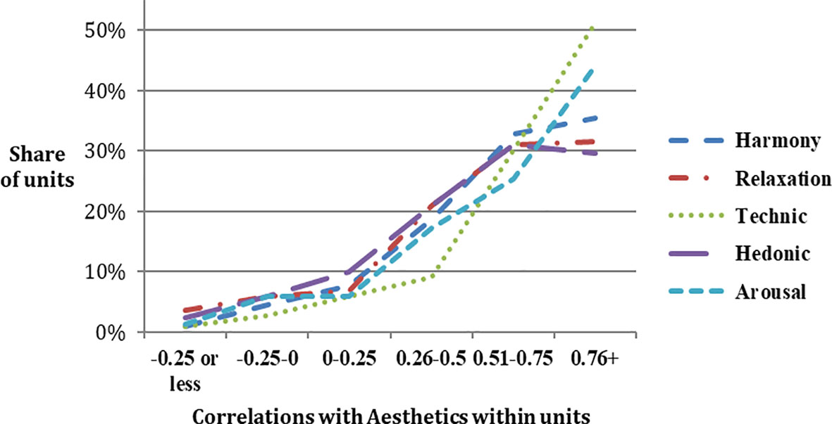

The regression model of price on all six aesthetic individual scores has no predictive power, with $R^{2}=$ 1%, that is in agreement with the previous findings. However, since the data has a complicated structure, we can consider it in more detail.

Figure 2 shows the unit-specific correlations of all aesthetic indicators and the logarithm of the Price, computed for all observed 220 units in the same fashion as it was employed for Fig. 1. These correlations are distributed for all variables very unevenly: about 30%–40% of the correlations for each indicator are negative, very few (1–5%) are more than 0.75), and about 20% exceed 0.5. For all data together, the correlations are 0.03–0.09, i.e., close to zero, but there are some individuals with quite high correlations.

Table 7 shows percent of negative correlations between the logarithm of price and different aesthetic indicators for each painter and for all units together. For example, 0.47 for Newman in column “Aesthetics” means that in 15 out of all 32 Newman’s units (47%) correlations between log (price) and aesthetic estimate were negative. Therefore, the expected relationship of “the better impression – the higher price” is not held almost in a half of the cases.

Table 7

Proportion of unit-specific negative correlations between Ln (price) and aesthetic indicators for different painters

	Number of units	Aesthetic	Harmony	Relaxation	Technique	Hedonic	Arousal	Average
Otto Dix	30	0.37	0.67	0.77	0.33	0.6	0.2	0.49
Barnett Newman	32	0.47	0.28	0.31	0.75	0.38	0.75	0.49
Joseph Turner	30	0.2	0.23	0.13	0.27	0.13	0.13	0.18
Caspar Friedrich	31	0.35	0.29	0.16	0.48	0.26	0.19	0.29
Joan Miro	30	0.2	0.27	0.23	0.33	0.2	0.2	0.24
Salvador Dali	30	0.3	0.5	0.23	0.23	0.3	0.33	0.32
Egon Schiele	11	0.45	0.36	0.09	0.45	0.36	0.55	0.38
Total/average	206	0.32	0.37	0.3	0.38	0.32	0.32	0.33

Figure 2.

Unit-specific correlations between Ln (Price) and of aesthetic indicators.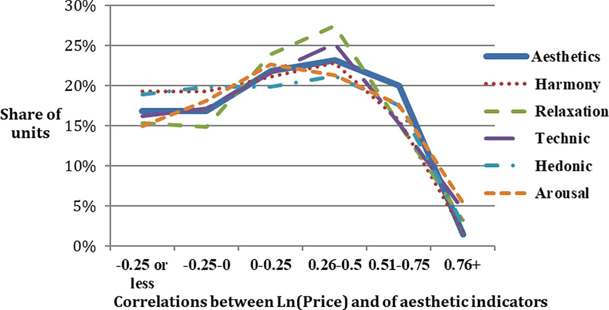

According to Table 7, 32%–38% of all units (the bottom row) are negatively correlated with the price. Dix, one of the most uncompromising artists ever, shows the highest level of negative coefficients (77%) for Relaxation, but one of the lowest (20%) for Arousal. Indeed, he is very far from conveying a “relaxing” atmosphere in his paintings, but he induces arousal and interest. The opposite is true for the very charming and more comprehensible Turner – all indicators reveal a very low percent of negative correlations, that could show that his irresistibly beautiful paintings produce a similar impression on buyers and on “commoners”. The average percent of negative correlations (the last column in Table 7) gives the idea of “level of apprehension” for a given artist: for example, Turner is the least inconsistent in the aesthetic impression and in pricing of his works, while Dix and Newman are the most controversial by this criterion. When respondents, unaware of the actual prices, give their aesthetics scores, but the prices are made in a different logic – then inevitably the correlations would be negative.

4. Conclusions

This research makes several contributions to the field of empirical aesthetics applied to painting. First, it has been shown that general aesthetic impression could be successfully modeled by more specific aesthetic indicators. Second, the hypothesis about strong interpretable correlation “price – aesthetics” was not supported by the data: the relation varies across different painters and groups of respondents and is absent in the whole population. What could be securely stated so far: the prices are higher for works which are interesting, relaxing, and not very technically elaborative. Third, the introduction of “units” (which resembles logic of the mixed models without dependent variable) looks promising for further studies, for it allows to separate the effects of the internal respondents’ feelings from the general trends, which could be misleading due to different scales used by respondents.

This work is just the beginning of a of a broader research program, and the paper outlines the research problems without offering the final answers. The future studies conducted on broader survey samplings could reveal how stable and correct the found relationships are. However, the directions of future research are clear: the more readers will visit the pollart1000.com to enter their scores, the better will be our understanding of the relations between the aesthetics variables and the prices of masterpieces discussed in the study.

Footnotes

Acknowledgments

Authors are grateful to Drs.: S. Lipovetsky who provided useful statistical references and helped in presenting the manuscript; G. Oksenoyt, who contributed to designing the questionnaire; V. Petrov who was very supportive on different stages of the project; I. Lipkovich for fruitful discussions; and to anonymous reviewers with very helpful comments. All errors and omissions are ours.

References

Amariglio

Childers

, & Cullenberg

eds, (2009). Sublime Economy: On the intersection of art and economics. New York: Routledge.

Anderson

(1974). Paintings as an investment. Economic Inquiry, 12, 13-26.

Austin

, & Steyerbergd

(2015). The number of subjects per variable required in linear regression analyses. Journal of Clinical Epidemiology, 68, 627-636.

Baumol

(1986). Unnatural value: Or art investment as floating crap game. The American Economic Review, 76(2), 10-14.

Birkhoff

G. D.

(1933). Aesthetic measure. Cambridge, MA: Cambridge Press.

Bocart

, & Hafner

(2012). Econometric analysis of volatile art markets. Computational Statistics & Data Analysis, 56(11), 3091-3104.

Boselie

, & Cesaro

(1994). Disjunctive ambiguity as a determinant of the aesthetic attractivity of visual patterns. Empirical Studies of the Arts, 12(1), 85-94.

Dutton

(2010). The art instinct: Beauty, pleasure, and human evolution. New York: Bloomsbury Press.

Feist

, & Brady

(2004). Openness to experience, nonconformity, and the preference for abstract art. Empirical Studies of the Arts, 22(1), 77-89.

10.

Ginsburgh

, & Weyers

(2009). On the contemporaneousness of Roger de Piles’ Balance des Peintres. in: Sublime Economy: On the Intersection of Art and Economics Amariglio

et al., eds, New York: Routlege, 112-124.

11.

Ginsburgh

, & Throasby

, eds, (2014). Handbook of the economics of art and culture. Oxford, UK: Elselvier.

12.

Goetzmann

Renneboog

, & Spaenjers

(2013). Art and money, https://papers.ssrn.com/sol3/papers.cfm?abstract_id=1501171.

13.

Heilbrun

, & Gray

(2004). The Economics of Art and Culture. 2nd ed. Cambridge, UK: Cambridge University Press.

14.

Korteweg

Kräussl

, & Verwijmeren

(2016). Does it Pay to Invest in Art? A Selection-corrected Returns Perspective. The Review of Financial Studies, 29(4), 1007-1038.

15.

Lipovetsky

, & Mandel

(2007). Humor and art: A topic for JSM’07. Amstat News, 355, 21.

16.

Lipovetsky

, & Mandel

(2009). How art helps to understand statistics. Model Assisted Statistics and Applications, 4(4), 313-324.

17.

Locher

P. J.

(2012). Empirical investigation of an aesthetic experience with art. in: Aesthetic science: Connecting Minds, Brains, and Experience, Oxford, UK: Oxford University Press Shimamura

A. P.

, & Palmer

S. E.

, eds, 163-188.

18.

Lopes

(2011). The myth of (non-aesthetic) artistic value. The Philosophical Quarterly, 61(244), 518-536.

19.

Mandel

, & Lipovetsky

(2007). Statistics in Humor and Art, roundtable # 216 at JSM’07. ASA Joint Statistical Meeting, July-August, Salt Lake City, UT, USA.

20.

Mandel

(2020). Aesthetic. Art-Historical and Economic Values in Painting: Empirical Study, https://papers.ssrn.com/sol3/papers.cfm?abstract_id=3160419.

21.

Marchi

(2009). Aesthetic and market value, 1708–1871. in: Sublime Economy: On the intersection of art and economics. Amariglio

et al., eds, New York: Routlege, 95-111.

22.

Marinelli

, & Palomba

(2010). A model for pricing italian contemporary art paintings at auction. The Quarterly Review of Economics and Finance, 51(2), 212-224.

23.

Marković

, & Radonjić

(2008). Implicit and explicit features of paintings. Spatial Vision, 21(3-5), 229-259.

24.

Mastandrea

Bartoli

, & Bove

(2009). Preferences for ancient and modern art museums: Visitor experiences and personality characteristics. Psychology of Aesthetics, Creativity, and the Arts, 3(3), 164-173.

25.

Mastandrea

Bartoli

, & Carrus

(2011). The automatic aesthetic evaluation of different art and architectural styles. Psychology of Aesthetic, Creativity, and the Arts, 5(2), 126-134.

26.

Mastandrea

, & Crano

(2019). Peripheral factors affecting the evaluation of artworks. Empirical Studies of the Arts, 37(1), 82-91.

27.

Mastandrea

Wagoner

J. A.

, & Hogg

M. A.

(2019). Liking for abstract and representational art: National identity as an art appreciation heuristic. Psychology of Aesthetics, Creativity, and the Arts. Advance online publication. doi: 10.1037/aca0000272.

28.

Murray

(2004). Human accomplishment: The pursuit of excellence in the arts and sciences, 800 B.C. to 1950. New York: Harper Perennial.

29.

Park

J. Y.

Park

J. H.

, & Park

J. H.

(2021). What type of title would you put on your paintings? The impact on the price of artwork according to its title. Empirical Studies of the Arts, 0(0), 1-24 doi: 10.1177/0276237421994700.

30.

Pénasse

Renneboog

, & Spaenjers

(2014). Sentiment and art prices. Economics Letters, 122(3), 432-434.

31.

Renneboog

, & Spaenjers

(2012). Buying beauty: On prices and returns in the art market. Management Science, 59(1), 36-53.

32.

Spaenjers

Goetzmann

W. N.

, & Mamonova

(2015). The economics of aesthetics and record prices for art since 1701. Explorations in Economic History, 57, 79-94.

33.

Spranzi

(2008). Economics & aesthetics: How can art economists obtain the aesthetic knowledge they need for their economic purposes? https://papers.ssrn.com/sol3/papers.cfm?abstract_id=1132997.

34.

Tansev

Kleiner

, & Croix

(1995). Gardner’s art through the ages. 10𝑡ℎ ed. Philadelphia, PA: Harcourt College.

35.

Teti

Galli

, & Sacco

(2014). Ephemeral estimation of the value of art. Empirical Studies of the Arts, 32(1), 75-92.

36.

Throasby

, & Zednik

(2014). The economical and cultural value of painting: Some empirical evidence. in: Handbook of the Economics of Art and Culture) Ginsburgh

, & Throasby

, eds, Oxford, UK: Elselvier, 2, 81-100.

37.

Turner

, eds, (1996). The Dictionary of Art, 34, New York: Grove.

	Number of respondents	Percent to total
Gender
Male	49	43%
Female	66	57%
Age
17–25	4	4%
25–34	46	40%
35–50	26	23%
51–64	23	20%
65 $+$	16	13%
Education
Higher school (graduated or not)	8	7%
Uncompleted bachelor, or associate degree	4	4%
Bachelor degree	14	12%
Graduated higher degrees	89	77%
Nationality
East Europe and Russia	52	45%
North America	42	37%
West Europe	14	12%
Other	7	6%
Relation to art
Art professional or strong interest in art	13	11%
Interested in art	61	53%
Don’t pay much attention to art	41	36%
Number of paintings rated by one respondent
$\geqslant$ 60	9	8%
21–59	25	22%
20	46	40%
5–18	14	12%
$<$ 5	21	18%
Total	115	100%

Beauty or money? Statistical analysis

Abstract

Keywords

1. Introduction

2. Data and survey design

2.1 The design of experiment

3.1 Artists with most evaluations

Table 2 Average aesthetic scores, prices, and correlations with general aesthetic impression

Table 3 Best and worst paintings for aesthetic indicators, average scores

Table 4 Pearson correlations between aesthetics and demographic variables

Footnotes

Acknowledgments

References

Table 2
Average aesthetic scores, prices, and correlations with general aesthetic impression

Table 3
Best and worst paintings for aesthetic indicators, average scores

Table 4
Pearson correlations between aesthetics and demographic variables