Different inference approaches for the estimators of the sushila distribution

Abstract

In this paper, we order to evaluate via Monte Carlo simulations the performance of sample properties of the estimates of the estimates for Sushila distribution, introduced by Shanker et al. (2013). We consider estimates obtained by six estimation methods, the known approaches of maximum likelihood, moments and Bayesian method, and other less traditional methods: L-moments, ordinary least-squares and weighted least-squares. As a comparison criterion, the biases and the roots of mean-squared errors were used through nine scenarios with samples ranging from 30 to 300 (every 30rd). In addition, we also considered a simulation and a real data application to illustrate the applicability of the proposed estimators as well as the computation time to get the estimates. In this case, the Bayesian method was also considered. The aim of the study was to find an estimation method to be considered as a better alternative or at least interchangeable with the traditional maximum likelihood method considering small or large sample sizes and with low computational cost.

Keywords

Bayesian analysis L-moments maximum likelihood method of moments Monte Carlo simulation ordinary least-squares weighted least-squares

1. Introduction

The Sushila distribution was introduced by Shanker et al. (2013). This distribution includes the one-parameter Lindley distribution (Ghitany et al., 2008; Lindley, 1958) as a particular case and can also be written as a mixture of distributions in the same way of the Lindley distribution. Its probability density function (pdf) is given by,

$\displaystyle f_{{X}}(x\mid\alpha,\theta)={\displaystyle\frac{\theta^{2}}{% \alpha(\theta+1)}}\left(1+{\displaystyle\frac{x}{\alpha}}\right)\exp\left\{-{% \displaystyle\frac{\theta}{\alpha}}x\right\},\quad x\in\mathbb{R}_{+},$ (1)

where $\theta\in\mathbb{R}_{+}$ is a scale parameter and $\alpha\in\mathbb{R}_{+}$ is a shape paramater. Shanker et al. (2013) showed that this model is a two-component mixture of an exponential distribution with scale parameter $\theta/\alpha$ and a gamma distribution having shape parameter 2 and scale parameter $\theta/\alpha$ with mixing proportion given by $\theta/(\theta+1)$ .

The mode of Sushila distribution is restricted to $0<\theta<1$ and is given by $\alpha(1-\theta)/\theta$ , that is, the Sushila distribution is unimodal only if $0<\theta<1$ , otherwise it is decreasing. A comprehensive discussion about the mathematical properties of the Sushila distribution such as moments, hazard function, stochastic orderings, parameter estimation, among others, is also presented by Shanker et al. (2013). Moreover, its discrete version was firstly introduced by Borah and Saikia (2016) based on the survival function proposed by Nakagawa and Osaki (1975); a second discrete version was introduced by de Oliveira et al. (2019) based on series method.

The corresponding cumulative distribution function (cdf) and survival function (sf) are given, respectively by,

$\displaystyle F_{{X}}(x\mid\alpha,\theta)=1-{\displaystyle\frac{\alpha(\theta+% 1)+\theta x}{\alpha(\theta+1)}}\exp\left\{-{\displaystyle\frac{\theta}{\alpha}% }x\right\}$ (2)

and,

$\displaystyle S_{{X}}(x\mid\alpha,\theta)={\displaystyle\frac{\alpha(\theta+1)% +\theta x}{\alpha(\theta+1)}}\exp\left\{-{\displaystyle\frac{\theta}{\alpha}}x\right\}$ (3)

The hazard function, according to Shanker et al. (2013), is an increasing function as the hazard function of the Lindley distribution and it is given by,

$\displaystyle h_{{X}}(x\mid\alpha,\theta)={\displaystyle\frac{\theta^{2}(% \alpha+x)}{\alpha[\alpha(\theta+1)+\theta x]}}$ (4)

For the estimation of the parameters of the Sushila distribution, Shanker et al. (2013) considered only maximum likelihood (ML) and moments (MO) estimation methods from where it could be seen that the moments estimator for $\theta$ is approximately the same as the maximum likelihood estimator. In this way, it could be interesting to compare the ML and MO estimators with some other estimate methods less traditional, the L-moments (LMO) estimation, ordinary least-squares (OLS) estimation and weighted least-squares (WLS) estimation, and also with Bayesian methods to decide which methods are more effective to get the inferences of interest for the Sushila distribution.

The main goal of this paper is to compare the six above cited different estimate methods via extensive simulation studies assuming complete data with small and large samples sizes. Another similar studies considring differents distributions can being see in, Kundu and Raqab (2005); Dey et al. (2014); Shawky and Bakoban (2012); Kim et al. (2010); Mazucheli et al. (2013); Teimouri et al. (2013) and others. This paper is organized as follows: In Section 2, it is discussed the six estimation methods considered in this paper. The comparison of these methods in terms of bias and root-mean-squared error as well applications involving simulated data are presented in Section 3. In Section 4, a real dataset is considered to compare the performance of the six estimation methods. Finally, in Section 5 it is presented some conclusions remarks and discussion of the obtained results.

2. Estimation methods

2.1 Maximum likelihood

Let $x_{1},x_{2},\ldots,x_{n}$ be a random sample of size $n$ from the Sushila distribution with parameters $\alpha$ and $\theta$ with pdf given by Eq. (1). Shanker et al. (2013) showed that the maximum likelihood estimators $\widehat{\alpha}_{ML}$ and $\widehat{\theta}_{ML}$ of $\alpha$ and $\theta$ are given by,

$\displaystyle\widehat{\theta}_{ML}={\displaystyle\frac{\widehat{\alpha}_{ML}-% \overline{X}+\sqrt{\overline{X}^{2}+6\overline{X}\widehat{\alpha}_{ML}+% \widehat{\alpha}_{ML}^{2}}}{2\overline{X}}}$ (5)

where $\overline{X}$ is the sample mean and $\widehat{\alpha}_{ML}$ is the solution of the non-linear equation:

$\displaystyle-{\displaystyle\frac{n}{\alpha}}+\sum_{x=1}^{n}{\displaystyle% \frac{x\mathsf{f}_{x}}{\alpha(\alpha+x)}}+{\displaystyle\frac{n\overline{X}% \widehat{\theta}_{ML}}{\alpha^{2}}}=0$ (6)

2.2 Method of moments

The method of moments is also traditional approach used in parameter estimation of a distribution. In this method is is necessary in order to understand the first moments of the distribution. Considering the Sushila distribution, we have to the first two raw moments are given, respectively, by,

$\displaystyle\mathbb{E}[X]={\displaystyle\frac{\alpha(\theta+2)}{\theta(\theta% +1)}}\quad\text{and}\quad\mathbb{E}[X^{2}]={\displaystyle\frac{2\alpha^{2}(% \theta+3)}{\theta^{2}(\theta+1)}}$ (7)

The methods of moments estimators $\widehat{\alpha}_{MO}$ and $\widehat{\theta}_{MO}$ for $\alpha$ and $\theta$ are obtained by solving the equations:

$\displaystyle{\displaystyle\frac{\alpha(\theta+2)}{\theta(\theta+1)}}=m_{1}% \quad\text{and}\quad{\displaystyle\frac{2\alpha^{2}(\theta+3)}{\theta^{2}(% \theta+1)}}=m_{2}$ (8)

where $m_{1}={\displaystyle\frac{1}{n}}\sum_{i=1}^{n}x_{i}$ is first sample moment and $m_{2}={\displaystyle\frac{1}{n}}\sum_{i=1}^{n}x_{i}^{2}$ is second sample moments.

2.3 Method of L-moments

The method of L-moments, is defined in terms of linear functions of population order statistics and their sample counterparts. This method was introduced by Hosking (1990). Considering the Sushila distribution, the first two population L-moments are, respectively, given by,

$\displaystyle L_{1}=\mathbb{E}[X_{1:1}]=\mathbb{E}[X]\quad\text{and}\quad L_{2% }={\displaystyle\frac{1}{2}}\mathbb{E}[X_{2:2}-X_{1:2}]=\mathbb{E}[X]-\mathbb{% E}[X_{1:2}]$ (9)

where $\mathbb{E}[X]$ is given by Eq. (7) and,

$\displaystyle\mathbb{E}[X_{1:2}]=\int_{0}^{\infty}[1-F_{{}_{X}}(x\mid\alpha,% \theta)]^{2}dx=\int_{0}^{\infty}\left[{\displaystyle\frac{\alpha(\theta+1)+% \theta x}{\alpha(\theta+1)}}\exp\left\{-{\displaystyle\frac{\theta}{\alpha}}x% \right\}\right]^{2}dx={\displaystyle\frac{\alpha(2\theta^{2}+6\theta+5)}{4% \theta(\theta+1)^{2}}}$ (10)

The L-moments estimators $\widehat{\alpha}_{\textit{LMO}}$ and $\widehat{\theta}_{\textit{LMO}}$ for $\alpha$ and $\theta$ are, respectively, obtained by solving the equations:

$\displaystyle{\displaystyle\frac{\alpha(\theta+2)}{\theta(\theta+1)}}=l_{1}% \quad\text{and}\quad{\displaystyle\frac{(2\theta^{2}+6\theta+3)\alpha}{4(% \theta+1)^{2}\theta}}=l_{2}$ (11)

where $l_{1}={\displaystyle\frac{1}{n}}\sum_{i=1}^{n}x_{i}$ and $l_{2}=\left[{\displaystyle\frac{2}{n(n+1)}}\sum_{i=1}^{n}(i-1)x_{i:n}\right]-{% \displaystyle\frac{1}{n}}\sum_{i=1}^{n}x_{i}$ are the first two sample L-moments.

2.4 Method of ordinary and weighted least-squares

Considering $x_{1:n}\leqslant\ldots\leqslant x_{n:n}$ the order statistics of a random sample of size $n$ derived on distribution with cdf $F(x)$ . So we known that:

$\displaystyle\mathbb{E}[F(x_{i:n})]={\displaystyle\frac{i}{n+1}}\quad\text{and% }\quad\text{Var}[F(x_{1:n})]={\displaystyle\frac{i(n-i+1)}{(n+1)^{2}(n+2)}}$ (12)

For the Sushila distribution, the least squares estimates $\widehat{\alpha}_{\textit{OLS}}$ and $\widehat{\theta}_{\textit{OLS}}$ for the parameters $\alpha$ and $\theta$ are, respectively, derived by minimizing the function,

$\displaystyle O(\alpha,\theta)=\sum_{i=1}^{n}\left[F(x_{i:n}\mid\alpha,\theta)% -\mathbb{E}[F(x_{i:n})]\right]^{2}=\sum_{i=1}^{n}\left[F(x_{i:n}\mid\alpha,% \theta)-{\displaystyle\frac{i}{n+1}}\right]^{2}$ (13)

On other hand, the weighted least-squares estimates $\widehat{\alpha}_{\textit{WLS}}$ and $\widehat{\theta}_{\textit{WLS}}$ for $\alpha$ and $\theta$ are, respectively, obtained by minimizing the function,

$\displaystyle W(\alpha,\theta)=\sum_{i=1}^{n}{\displaystyle\frac{\left[F(x_{i:% n}\mid\alpha,\theta)-\mathbb{E}[F(x_{i:n})]\right]^{2}}{\text{Var}[F(x_{1:n})]% }}=\sum_{i=1}^{n}{\displaystyle\frac{(n+1)^{2}(n+2)}{i(n-i+1)}}\left[F(x_{i:n}% \mid\alpha,\theta)-{\displaystyle\frac{i}{n+1}}\right]^{2}$ (14)

where the cdf of the order statistics, $F(x_{i:n},\alpha,\theta)$ , for the Sushila distribution is given by,

$\displaystyle F(x_{i:n}\mid\alpha,\theta)=\sum_{r=i}^{n}{n\choose r}\left[1-{% \displaystyle\frac{\alpha(\theta+1)+\theta x}{\alpha(\theta+1)}}\exp\left\{-{% \displaystyle\frac{\theta}{\alpha}}x\right\}\right]^{r}\left[{\displaystyle% \frac{\alpha(\theta+1)+\theta x}{\alpha(\theta+1)}}\exp\left\{-{\displaystyle% \frac{\theta}{\alpha}}x\right\}\right]^{n-r}$ (15)

2.5 Bayesian estimation method

In order to determine the Bayesian estimators for the unknown parameters of the Sushila distribution based on the squared error loss function, $L(\eta,a)=(\eta-a)^{2}$ , suppose that the parameters $\alpha$ and $\theta$ have independent gamma prior distributions with same hyperparater values given respectively, by,

$\displaystyle\pi_{1}(\alpha)={\displaystyle\frac{\beta^{\lambda}}{\Gamma(% \lambda)}}\alpha^{(\lambda-1)}\exp\{-\beta\alpha\}\quad\text{and}\quad\pi_{2}(% \theta)={\displaystyle\frac{\beta^{\lambda}}{\Gamma(\lambda)}}\theta^{(\lambda% -1)}\exp\{-\beta\theta\}.$ (16)

Such that, the gamma distribution with mean $\lambda/\beta$ and variance $\lambda/\beta^{2}$ . In this case, the joint posterior density function for the Sushila distribution is given by,

$\displaystyle\pi(\alpha,\theta\mid\textbf{x})\propto\left[{\displaystyle\frac{% \beta^{2\lambda}\theta^{2}}{\alpha(\theta+1)[\Gamma(\lambda)]^{2}}}\right]% \alpha^{\lambda-1}\theta^{\lambda-1}\exp\{-\beta(\alpha+\theta)\}\prod_{i=1}^{% k}\left(1+{\displaystyle\frac{x_{i}}{\alpha}}\right)^{\mathsf{f}_{x_{i}}}\exp% \left\{-{\displaystyle\frac{n\theta}{\alpha}}\overline{x}\right\}$ (17)

where $\mathsf{f}_{x}$ is the observed frequency in the sample corresponding to $X=x,(x=1,2,\ldots,k)$ such that $\sum_{x=1}^{k}\mathsf{f}_{x}=n$ where $k$ is the largest observed value having non-zero frequency; and $\beta,\lambda$ are positive real numbers. The values for the hyperparameters $\beta$ and $\lambda$ were chosen in order to reflect prior knowledge of the parameters and better performance of the algorithm in terms of good convergence and computation stability. In general the values $\beta$ and $\lambda$ of are chosen to obtain mean prior equal to 1 and high variance, thus becomes a prior distribution approximately non-informative. In this paper, without loss of generality, it is used the Gibbs sampling algorithm (Gelfand & Smith, 1990; Casella & George, 1992) to generate samples from the posterior distribution of interest from which it is computed the Monte Carlo Bayes estimators (Bayes) under the squared error loss function. The Gibbs sampling algorithm steps are given by,

•

Step 1: Choose initial values, $\alpha^{(0)}$ and $\theta^{(0)}$ for $\alpha$ and $\theta$ . Denote the values of $\alpha$ and $\theta$ at the $i^{\text{th}}$ step by $\alpha^{(i)},\theta^{(i)}$ .

•

Step 2: Generate $\alpha^{(i)}$ , $\theta^{(i+1)}$ from the conditional posterior distributions needed for the Gibbs sampling algorithm obtained directly from the joint posterior distribution.

•

Step 3: Repeat step 2, $N$ times.

•

Step 4: Calculate the Monte Carlo Bayes estimate of $\omega(\alpha,\theta)$ using the expression given by $(1/(N-B))\linebreak{\sum}_{i=B+1}^{N}\omega(\alpha^{(i)},\theta^{(i)})$ where $B$ is the burn-in period.

To simulate samples from the joint posterior distribution, we could consider the use of algorithms implemented in the JAGS software (Plummer, 2003), where we just need to specify the data distribution and the prior distribution for the parameters.

3. Generation algorithms and monte carlo simulation study

3.1 Generation algorithms

In this subsection, two different algorithms for generating random data from the Sushila distribution are presented as follows:

1.
The first algorithm is based on generating random data from Sushila distribution using the exponential-gamma mixture form;
2.
The second algorithm is based on generating random data from the inverse cdf in Eq. (2) of the Sushila distribution.

Algorithm 1: (mixture form of the Sushila distribution)

1. Generate $U_{i}\sim\textit{Uniform}(0,1),i=1,\ldots,n;$

2. Generate $V_{i}\sim\textit{Exponential}(\theta/\alpha),i=1,\ldots,n;$

3. Generate $W_{i}\sim\textit{Gamma}(2,\theta/\alpha),i=1,\ldots,n;$

4. If $U_{i}\leqslant{\displaystyle\frac{\theta}{\theta+1}}$ , then set $X_{i}=V_{i}$ , otherwise, set $X_{i}=W_{i},i=1,\ldots,n.$

Algorithm 2: (inverse cdf)

1. Generate $U_{i}\sim\textit{Uniform}(0,1),i=1,\ldots,n;$

2. Set
$\displaystyle X_{i}=-\alpha-{\displaystyle\frac{\alpha}{\theta}}-{% \displaystyle\frac{\alpha}{\theta}}W_{-1}((u-1)(\theta+1)\exp\{-1-\theta\}),i=% 1,\ldots,n,$ (18) where $W_{-1}(\cdot)$ denotes the negative branch of the Lambert W function (Jodrá, 2010; Lambert, 1758).

3.2 Simulation results

Algorithm 1: (mixture form of the Sushila distribution)
1. Generate $U_{i}\sim\textit{Uniform}(0,1),i=1,\ldots,n;$
2. Generate $V_{i}\sim\textit{Exponential}(\theta/\alpha),i=1,\ldots,n;$
3. Generate $W_{i}\sim\textit{Gamma}(2,\theta/\alpha),i=1,\ldots,n;$
4. If $U_{i}\leqslant{\displaystyle\frac{\theta}{\theta+1}}$ , then set $X_{i}=V_{i}$ , otherwise, set $X_{i}=W_{i},i=1,\ldots,n.$

Algorithm 2: (inverse cdf)
1. Generate $U_{i}\sim\textit{Uniform}(0,1),i=1,\ldots,n;$
2. Set $\displaystyle X_{i}=-\alpha-{\displaystyle\frac{\alpha}{\theta}}-{% \displaystyle\frac{\alpha}{\theta}}W_{-1}((u-1)(\theta+1)\exp\{-1-\theta\}),i=% 1,\ldots,n,$ (18) where $W_{-1}(\cdot)$ denotes the negative branch of the Lambert W function (Jodrá, 2010; Lambert, 1758).

This subsection reports the results of a simulation study carried out to assess the performance of the ML, Bayes, MO, LMO, OLS and WLS estimators for the Sushila distribution assuming complete data. The simulation study was performed in R (R Core Team, 2018) software using the packages maxLik (Henningsen & Toomet, 2011) for ML estimators, nleqslv (Hasselman, 2018) for MO and LMO estimators and optim function for OLS and WLS estimators. The Broyden-Fletcher-Goldfarb-Shanno (BFGS) and Newton optimization methods were considered as optim.method. For the Bayesian approach, the R2jags package (Su & Yajima, 2015) was considered to get the inferences of interest, and we assumed approximately non-informative gamma prior distributions with hyperparameter values equal to (0.001, 0.001). Also, the Algorithm 2 (inverse cdf) was considered to generate random samples from the Sushila distribution.

The simulation study was performed under nine scenarios considering the assumed parameter values as the combination of $\alpha\times\theta=(0.3,0.6,0.9)\times(0.3,0.6,0.9)$ for better computational stability. It was also considered the sample sizes $n=30,60,\ldots,300$ , each one involving 10,000 Monte Carlo replications. For each scenario, the biases (BIAS) and the root of the mean squared errors (RMSE) for the estimated parameter component of the vector of parameters $(\alpha,\theta)$ were respectively computed using the expressions:

$\displaystyle\textit{BIAS}(\widehat{\Psi})=\frac{1}{N}\sum_{i=1}^{N}(\widehat{% \Psi}_{i}-\Psi)\text{ and }\textit{RMSE}(\widehat{\Psi})=\sqrt{\frac{1}{N}\sum% _{i=1}^{N}(\widehat{\Psi}_{i}-\Psi)^{2}}$

where $N=$ 10,000 is the number of simulations and $\Psi$ denotes each parameter $\alpha$ or $\theta$ . From the simulation results, it is possible to conclude that,

i.)
Assuming the ML estimators of both parameters, it could be seen that the ML estimators are asymptotically non-biased since $E(\theta)\approx\theta$ and $E(\alpha)\approx\alpha$ when $n\rightarrow\infty$ . Moreover, the RMSE values also tend to zero when $n\rightarrow\infty$ . Compared to the others, the ML estimator is close to the Bayes estimator to get the inferences of interest for Sushila distribution and, for this estimator, the biases and RMSEs values are lower than obtained from the other methods (except Bayes estimator).
ii.)
Assuming the Bayes estimators of both parameters, it could be seen that the Bayes estimators are asymptotically non-biased for the parameter $\alpha$ since $E(\alpha)\approx\alpha$ and it is seen negative biased in one scenario when $n\rightarrow\infty$ for parameter $\theta$ when $n\rightarrow\infty$ . Compared to the others, the Bayes estimator is not so good as the ML estimator to get the inferences of interest for Sushila distribution, however, this estimator depends on the choice of a prior distribution that could provide better results for the biases and RMSEs. That is, the Bayes estimator could be an useful estimator as the ML, MO, LMO estimators in practice.
iii.)
Assuming the MO estimators of both parameters, it could be seen that the MO estimators are asymptotically non-biased since $E(\theta)\approx\theta$ and $E(\alpha)\approx\alpha$ when $n\rightarrow\infty$ . Moreover, the RMSE values also tend to zero when $n\rightarrow\infty$ .
iv.)
In the same way of MO estimators for both parameters, it could be seen that the LMO estimators are asymptotically non-biased since $E(\theta)\approx\theta$ and $E(\alpha)\approx\alpha$ when $n\rightarrow\infty$ . Moreover, the RMSE values also tend to zero when $n\rightarrow\infty$ . However, compared to the MO estimator, the LMO estimator is a little more unstable which reduces its performance.
v.)
Assuming the OLS estimators, it could be seen that the OLS estimator for $\alpha$ is negative biased and the OLS estimator for $\theta$ is positive biased, that is, $E(\theta)\neq\theta$ and $E(\alpha)\neq\alpha$ when $n\rightarrow\infty$ . Considering the RMSE values, it could be seen that the RMSE do not tend to zero when $n\rightarrow\infty$ , in fact, it seems almost constant. In conclusion, the OLS estimator is not a good choice for the estimation of the parameters of the Sushila distribution.
vi.)
In the same way as for the OLS estimators, it could be seen that the WLS estimator for $\alpha$ is negative biased and the WLS estimator for $\theta$ is positive biased, that is, $E(\theta)\neq\theta$ and $E(\alpha)\neq\alpha$ when $n\rightarrow\infty$ . Considering the RMSE values, it could be seen that the RMSE do not tend to zero when $n\rightarrow\infty$ , in fact, it seems almost constant. In conclusion, the WLS estimator also is not a good choice for the estimation of the parameters of the Sushila distribution.
vii.)
Based on these simulation results and using the Algorithm 2 to generate the simulated data, it could be concluded that the MO, LMO, Bayes and MLE estimators are the best estimators to get inferences of interest assuming the Sushila distribution due to their performance in the simulation studies and the fact that they are not biased when the sample size increases and the RMSE values tend to zero, mainly observed in MLE and Bayes estimators. The OLS and WLS should not be used to get estimators for the parameters of the Sushila since these estimators could be strongly biased. In conclusion, the Sushila distribution could be used as good alternative to other existing continuous univariate distributions to describe univariate lifetimes with good accuracy if the MO, LMO, Bayes and MLE estimators are considered; also, the results could be improved assuming the Algorithm 1 to generate the random data.

Figure 1.
The biases and RMSEs for both parameters assuming the Sushila distribution for each considered scenario considering the ML estimators assuming complete data (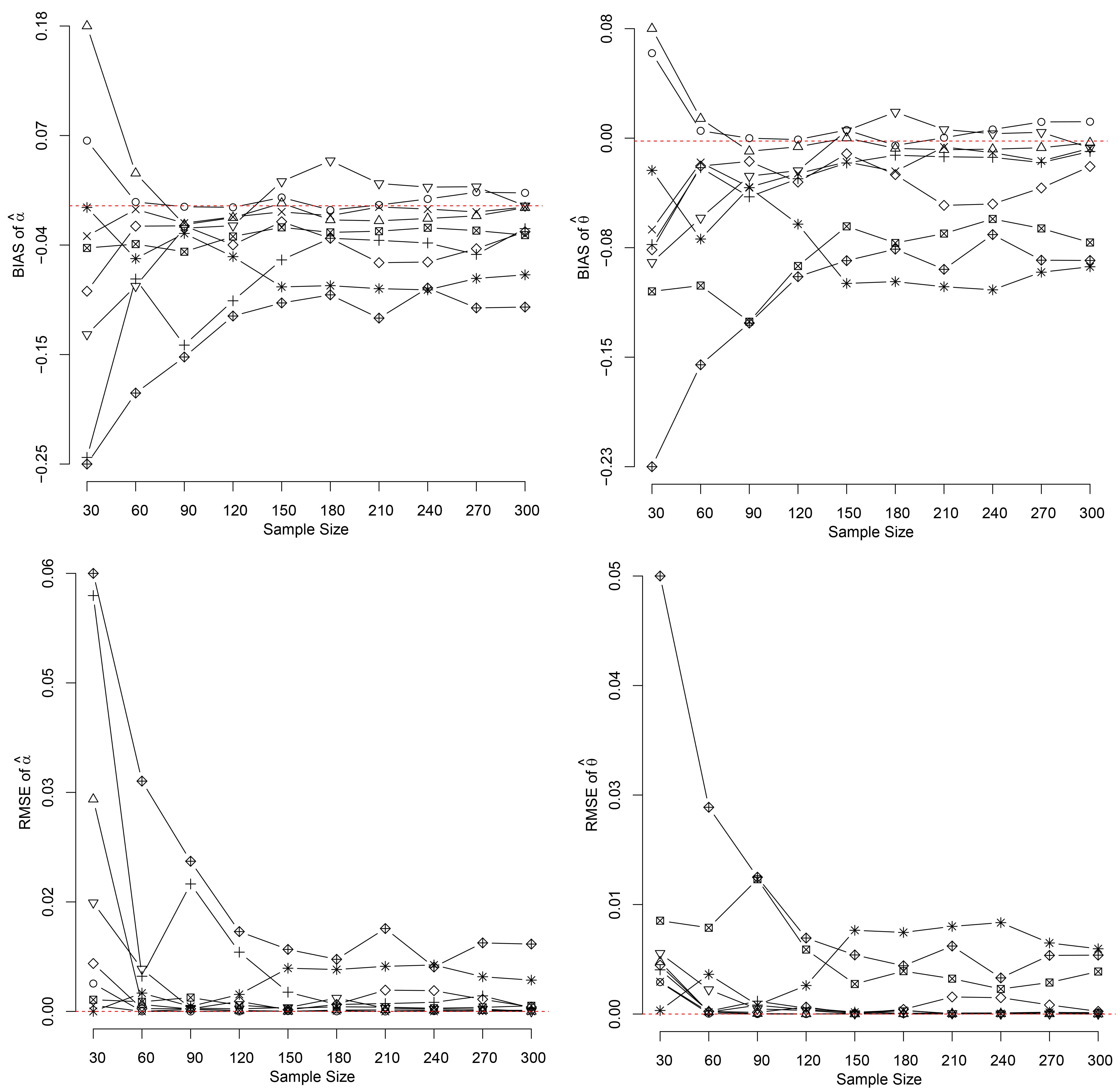 $\circ:(\alpha=0.3,\theta 0.3)$ ; $\triangle:(\alpha=0.6,\theta=0.3)$ ; $+:(\alpha=0.9,\theta=0.3)$ ; $\times:(\alpha=0.3,\theta=0.6)$ ; $\diamond:(\alpha=0.6,\theta=0.6)$ ; $\triangledown:(\alpha=0.9,\theta=0.6)$ ; $\boxtimes:(\alpha=0.3,\theta=0.9)$ ; $\ast:(\alpha=0.6,\theta=0.9)$ ; $\Diamond$ $+$ : $(\alpha=0.9,\theta=0.9)$ ).

Figure 2.
The biases and RMSEs for both parameters assuming the Sushila distribution for each considered scenario considering the Bayes estimators assuming complete data (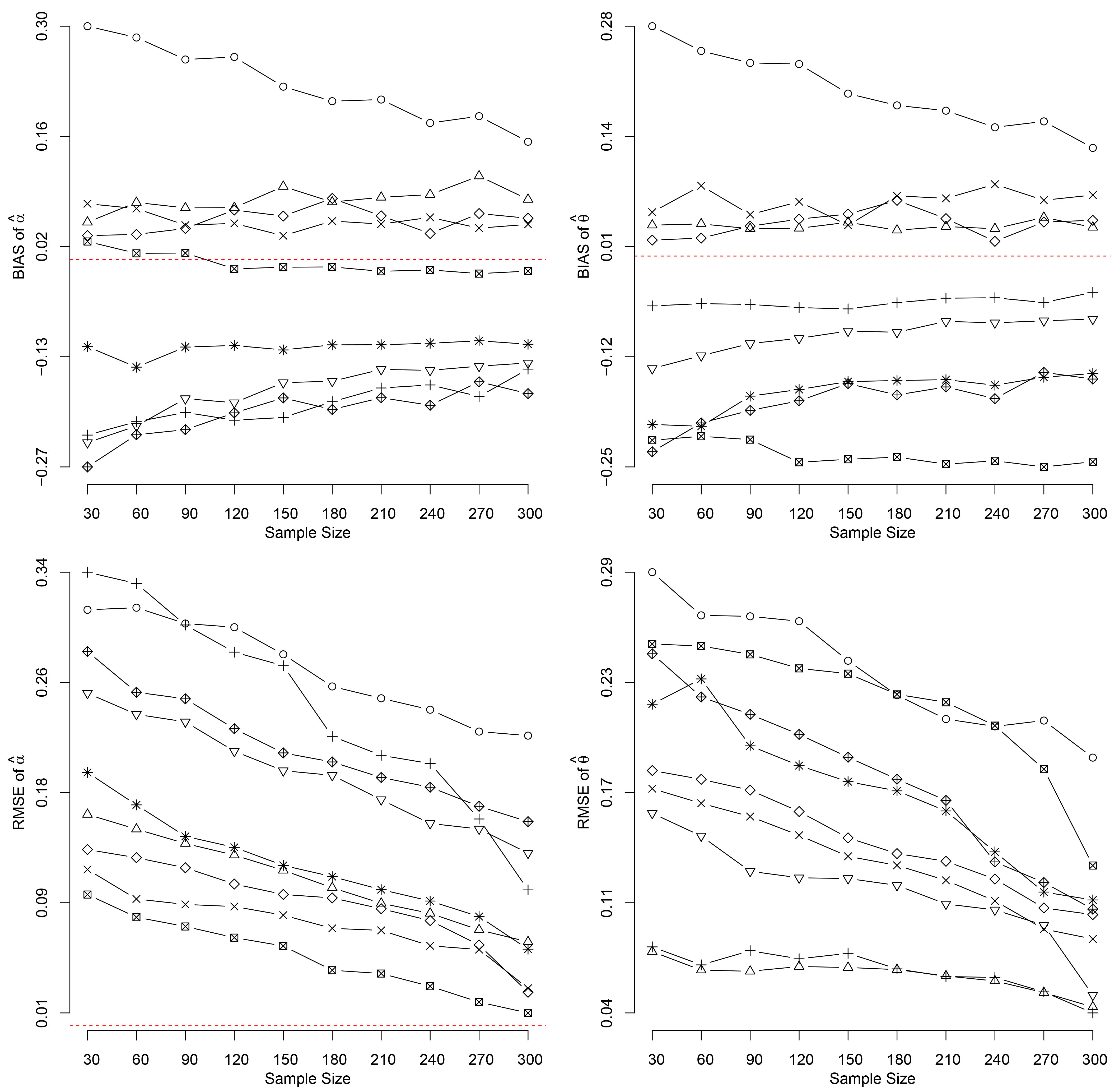 $\circ:(\alpha=0.3,\theta 0.3)$ ; $\triangle:(\alpha=0.6,\theta=0.3)$ ; $+:(\alpha=0.9,\theta=0.3)$ ; $\times:(\alpha=0.3,\theta=0.6)$ ; $\diamond:(\alpha=0.6,\theta=0.6)$ ; $\triangledown:(\alpha=0.9,\theta=0.6)$ ; $\boxtimes:(\alpha=0.3,\theta=0.9)$ ; $\ast:(\alpha=0.6,\theta=0.9)$ ; $\Diamond$ $+$ : $(\alpha=0.9,\theta=0.9)$ ).

The obtained simulation results for each scenario of the best estimators assuming complete data are illustrated in Figs 1 and 2 for ML and Bayes, respectively.
3.3 A numerical experiment

Let us consider now $n=50$ univariate lifetimes generated from the Sushila distribution using the Algorithm 2 (dataset in Table 1) with nominal parameters values $\alpha=0.3$ and $\theta=0.7$ to evaluate the performance of the proposed estimators in Section 2 for the Sushila distribution. In this experiment, we aim to assess how close the proposed estimators get to the nominal values.

For the statistical analysis, it is considered all methods of estimation presented in Section 2, and for Bayesian approach, we assumed approximately non-informative uniform prior distributions with hyperparameter values equal to (0, 1) instead of gamma (0.001, 0.001) prior distributions. The results are presented in Table 2, and as comparative criteria, we considered the highest $p$ -value of the Anderson-Darling (AD) test and the highest $p$ -value of the Cramer-Von Mises (CvM) test. The null-hypothesis of these tests is that the provided data follow a Sushila distribution with the estimated parameters.

Table 1
Simulated lifetimes from a Sushila distribution with nominal parameters values $\alpha=0.3$ and $\theta=0.7$

$X$	0.28814033	1.04722669	0.42074421	1.37376358	1.73042181	0.04649650	0.56931812
	1.41874240	0.60156574	0.47737233	1.89614044	0.47336685	0.80369526	0.63201302
	0.10345411	1.45684891	0.24553437	0.04298062	0.33069754	1.86918975	1.40458661
	0.83238738	0.73839779	2.90040954	0.76445815	0.86331939	0.59124365	0.66414873
	0.28978658	0.14693287	1.97520496	1.47017107	0.82836421	1.06663647	0.02532433
	0.50365116	0.97220180	0.21561737	0.32030635	0.23090667	0.14268757	0.42720400
	0.42624807	0.37529833	0.15218196	0.13875807	0.23232672	0.48887895	0.26582569
	1.26808188

Table 2

Inference summaries for Sushila distribution with nominal parameters values $\alpha=0.3$ and $\theta=0.7$

Method	Estimates	AD	CvM
		$p$ -values
ML	$\widehat{\alpha}=$ 0.2614	0.9843	0.9537
	$\widehat{\theta}=$ 0.5833
BAYES	$\widehat{\alpha}=$ 0.3384	0.9522	0.9673
	$\widehat{\theta}=$ 0.6698
MO	$\widehat{\alpha}=$ 0.2681	0.9234	0.8175
	$\widehat{\theta}=$ 0.5837
LMO	$\widehat{\alpha}=$ 0.4113	0.8787	0.7548
	$\widehat{\theta}=$ 0.8644
OLS	$\widehat{\alpha}=$ 0.0658	0.0006	$<$ 0.0001
	$\widehat{\theta}=$ 0.9497
WLS	$\widehat{\alpha}=$ 0.0463	0.0005	$<$ 0.0001
	$\widehat{\theta}=$ 0.9947

From the results of Table 2 and by comparison of the obtained estimates with the to the true parameter values adopted in this simulated dataset, it is possible to conclude that the ML and Bayes methods satisfies the adopted criteria, that is, highest $p$ -values for the AD and CvM tests. For MO and LMO estimation methods, we also can see that, according to CvM test, that those obtained estimators are quite good compared to the ML and Bayes estimates which is expected in the simulation study. Finally, for OLS and WLS estimation methods, we obtained the expected behavior (positive biased for $\theta$ and negative biased for $\alpha$ ) for the estimates as pointed out in the simulation study. In conclusion, the maximum likelihood and Bayesian estimation methods are the most adequate among the six considered estimation methods to get the inferences of interest for the Sushila distribution.

4. Real data example

Now, to close our study of the proposed inference methods for Sushila distribution, let us consider a real dataset related to lifetimes of 20 electronic components introduced by Razali and Salih (2009) (dataset in Table 1) to evaluate the performance of the proposed estimators in a real data situation. For the statistical analysis, it is considered all methods of estimation presented in Section 2 and for the Bayesian approach we assumed approximately non-informative gamma prior distributions with hyperparameter values equal to gamma (0.001, 0.001). The results are presented in Table 2, and as comparative criteria, we considered the highest $p$ -value of the Anderson-Darling (AD) test and the highest $p$ -value of the Cramer-Von Mises (CvM) test.

Table 3
Lifetimes of 20 electronic components

0.03	012	0.22	0.35	0.73
0.79	1.25	1.41	1.52	1.79
1.8	1.94	2.38	2.4	2.87
2.99	3.14	3.17	4.72	5.09

Table 4

Inference summaries for Sushila distribution assuming the lifetimes of 20 electronic components data

		$p$ -values
Method	Estimates	AD	CvM
ML	$\widehat{\alpha}=$ 2.1413	0.8560	0.9685
	$\widehat{\theta}=$ 1.2268
BAYES	$\widehat{\alpha}=$ 2.1160	0.8981	0.9775
	$\widehat{\theta}=$ 1.2236
MO	$\widehat{\alpha}=$ 3.4726	0.6073	0.6501
	$\widehat{\theta}=$ 1.2273
LMO	$\widehat{\alpha}=$ 4.9726	0.6119	0.5773
	$\widehat{\theta}=$ 2.5237
OLS	$\widehat{\alpha}=$ 2.7581	0.0412	0.0053
	$\widehat{\theta}=$ 0.6523
WLS	$\widehat{\alpha}=$ 2.7579	0.0293	0.0093
	$\widehat{\theta}=$ 0.6280

From the obtained results of Table 4, it is possible again, to conclude that the ML and Bayes methods satisfies the adopted criteria, that is, highest $p$ -values of the AD and CvM tests. Both methods present close values for the parameter estimates, different of the other methods from where we can see that the values of the parameter estimates are far from the ML and Bayes estimates. This result is expected, according to the simulation study. Also, the MO and LMO estimation methods could be an alternative to ML and Bayes in this case, however, they could provide quite accurate information in this case due to the difference between MO and ML/Bayes or LMO and ML/Bayes. Finally, for the OLS and WLS estimation methods, we obtained values close to the ML and Bayes estimators, however, according to the adopted criteria, those estimators are worse for this dataset which is expected according to our simulation study. In conclusion, the maximum likelihood and Bayesian estimation methods are the most adequate among the six considered estimation methods for Sushila distribution.

5. Concluding remarks

The present study sought to compare by extensive simulation experiments, the efficiency of estimation of the parameters of the Sushila distribution considering six well-known estimation methods. The methods used in this paper were, the maximum likelihood, the method of moments, the method of L-moments, ordinary and weighted least-squares, and the Bayesian method. The simulation study concludes that the maximum likelihood and Bayesian methods are highly recommended for most practical sample sizes. The simulation study also showed that the ordinary least-squares and weighted least-squares inference methods are not recommended for the Sushila distribution since those estimators are biased. This is supported by the analysis of the real data analysis presented in Section 4 of this manuscript.

References

Borah

, & Saikia

K.R.

(2016). Certain properties of discrete Sushila. Statistics, 5(6).

Casella

, & George

E.I.

(1992). Explaining the Gibbs sampler. The American Statistician, 46(3), 167-174.

de Oliveira

R.P.

de Oliveira Peres

M.V.

Martinez

E.Z.

, & Achcar

J.A.

(2019). Use of a discrete Sushila distribution in the analysis of right-censored lifetime data. Model Assisted Statistics and Applications, 14(3), 255-268.

Dey

, & Kundu

(2014). Two-parameter Rayleigh distribution: Different methods of estimation. American Journal of Mathematical and Management Sciences, 33(1), 55-74.

Gelfand

A.E.

, & Smith

A.F.

(1990). Sampling-based approaches to calculating marginal densities. Journal of the American Statistical Association, 85(410), 398-409.

Ghitany

M.E.

Atieh

, & Nadarajah

(2008). Lindley distribution and its application. Mathematics and Computers in Simulation, 78(4), 493-506.

Hasselman

(2018). nleqslv: Solve Systems of Nonlinear Equations. R package version 3.3.2.

Henningsen

, & Toomet

(2011). maxlik: A package for maximum likelihood estimation in R. Computational Statistics, 26(3), 443-458.

Hosking

J.R.

(1990). L-moments: analysis and estimation of distributions using linear combinations of order statistics. Journal of the royal statistical society. Series B (Methodological), pages 105–124.

10.

Jodrá

(2010). Computer generation of random variables with Lindley or Poisson-Lindley distribution via the Lambert W function. Mathematics and Computers in Simulation, 81(4), 851-859.

11.

Kim

S.-I.

Park

M.-Y.

, & Park

J.-W.

(2010). A comparison of estimation methods for Weibull distribution and type I censoring. Journal of the Korean Society for Quality Management, 38(4), 480-490.

12.

Kundu

, & Raqab

M.Z.

(2005). Generalized Rayleigh distribution: Different methods of estimations. Computational Statistics & Data Analysis, 49(1), 187-200.

13.

Lambert

J.H.

(1758). Observationes variae in mathesin puram. Acta Helvetica, 3(1), 128-168.

14.

Lindley

D.V.

(1958). Fiducial distributions and Bayes’ theorem. Journal of the Royal Statistical Society. Series B (Methodological), pages 102–107.

15.

Mazucheli

Louzada

, & Ghitany

(2013). Comparison of estimation methods for the parameters of the weighted Lindley distribution. Applied Mathematics and Computation, 220, 463-471.

16.

Nakagawa

, & Osaki

(1975). The discrete Weibull distribution. IEEE Transactions on Reliability, 24(5), 300-301.

17.

Plummer

(2003). Jags: A program for analysis of bayesian graphical models using gibbs sampling.

18.

R Core Team (2018). R: A Language and Environment for Statistical Computing. R Foundation for Statistical Computing, Vienna, Austria.

19.

Razali

A.M.

, & Salih

A.A.

(2009). Combining two weibull distributions using a mixing parameter. European Journal of Scientific Research, 31(2), 296-305.

20.

Shanker

Sharma

Shanker

, & Shanker

(2013). Sushila distribution and its application to waiting times data. International Journal of Business Management, 3(2), 1-11.

21.

Shawky

, & Bakoban

R.A.

(2012). Exponentiated gamma distribution: Different methods of estimations. Journal of Applied Mathematics, 2012.

22.

Y.-S.

, & Yajima

(2015). R2jags: Using R to Run ’JAGS’. R package version 0.5-7.

23.

Teimouri

Hoseini

S.M.