An EM model for analysis of discrete time competing risks data with missing failure causes

Abstract

Larson and Dinse (1985) have introduced the mixture model as an additional competing risks model. In the same article, the authors have suggested that this model can be upscaled to handle the presence of missing failure causes in data. We respond to this proposal in this article and develop a regression model for analysis of data that comes with this complication. We also demonstrate that, with minimal adjustments, the proposed model can be applied in discrete time. This development will be of benefit to discrete time competing risks as analysis of data with this complication is a subject that has not received adequate attention. The mixture model has two components, the incidence and the latency component. It is demonstrated that the parameters related to the model for the latency component as proposed by Larson and Dinse (1985) can be estimated by applying a certain Poisson regression.

Keywords

Missing failure causes mixture competing risks model discrete time competing risks poisson regression model

1. Introduction

Competing risks refers to survival analysis experiments where there are multiple modes of failure. In some instances data from these experiments may come with subjects that have failed with unknown failure causes. A number of reasons may lead to this data complication in practice. In clinical trials, for example, Anderson et al. (1996) cite lack of requisite instrumentation to determine the cause of death or negligence on the part of recording clerks to capture a known cause of failure etc., as some of the reasons that may lead to this data complication. The standard analysis methods such as modelling competing risks data with cause-specific-hazards via Cox (1972) regression model are no longer applicable in the presence of missing failure causes. Larson and Dinse (1985) have suggested the mixture competing risks model as an alternative to the cause-specific-hazards model (Prentice et al., 1978). In the same article, Larson and Dinse (1985) have proposed that their model can be upscaled to handle missing failure causes. The primary objective of this article is to demonstrate that, indeed, the model can be extended to deal with missing failure cause. More importantly, we demonstrate how the proposed model can be applied in discrete time with minimal adjustments regarding failure/censoring times. Analysis of data that comes with missing failure causes is a topic that has been widely discussed in the competing risks literature, however, the development of models to deal with this data complication have taken place almost exclusively in the continuous time realm, see for example, (Dinse, 1982; Dewanji, 1992; Goetghebeur & Ryan, 1990, 1995; Lu & Tsiatis, 2001; Nicolaie et al., 2015). Discrete time models in general have not received the same attention as continuous time models. The existing discrete time regression models (Ambrogi et al., 2009; Tutz & Schmid, 2016; Lee et al., 2018) cannot handle missing failure causes because they all advance cause-specific-hazards for modelling data. The estimation of cause-specific-hazards requires full information regarding failure causes for all failures. The application of these models is limited to ad hoc methods, that is, data is edited by, for example, creating an additional failure mode for the affected subjects or excluding them from analysis before these models can be considered for application. Ad hoc methods are not ideal as they tend to produce downward biased estimates for cause-specific-hazards (Anderson et al., 1996).

Suppose that $C$ denotes time to censoring. In the absence of missing failure causes, observed data on the pair $(\tilde{T};D)$ with covariates can be represented by $\bm{y}=((t_{1},\epsilon_{1},\bm{x}_{1}),\dots(t_{n},\epsilon_{n},\bm{x}_{n}))^% {T}$ due to $C_{i}$ , where $T_{i}=\tilde{T}_{i}\wedge C_{i}$ , and $\epsilon_{i}=I(\tilde{T}_{i}<C_{i})D_{i}$ . The subject $i$ covariates are collected in a $p$ -dimensional vector $\bm{x}_{i}$ . Over the years, modelling competing risks data with cause-specific-hazards via the Cox (1972) proportional hazards assumption has been the dominant regression analysis method;

$\displaystyle h_{j}(t|\bm{x};\bm{\phi}_{j})=h_{0j}(t)\exp(\bm{x}^{T}\bm{\phi}_% {j})$ (1)

for $j=1,2\dots J$ . On the other hand, the mixture model proposes $\lambda_{j}(t)\,(j=1,2,\dots J)$ and failure type probabilities $\pi_{j}(t)(j=1,2,\dots J)$ for modelling observed data. Characterizing data with component hazards and failure type probabilities follows from the mixture model assumption which proposes a decomposition of the bivariate distribution $(\tilde{T},D)$ into a marginal distribution for failure type (incidence) and a time to failure distribution conditional on failure type (latency). The model assumes that observed data has come from a mixed population with $J$ supopulations each with its own failure time distribution. Therefore, $\lambda_{j}(t)(j=1,2,\dots J)$ is the hazard function for failure times due to failure cause $j$ and the censored failure times that are destined to fail due to failure cause $j$ . The model allows for flexibility in the choice of a model for the component hazards. When Larson and Dinse (1985) introduced the model, they assumed proportional hazards for component hazards with piece-wise constant baseline component hazards;

$\displaystyle\lambda_{j}(t|\bm{x};\bm{\beta}_{j})=\exp\left(\sum_{s=1}^{q}% \beta_{0js}I(s\in[a_{t-1},a_{t}])+\bm{x}^{T}\bm{\beta}_{1j}\right)$ (2)

where $\bm{\beta}_{0j}=(\beta_{0j1},\beta_{0j2}\dots\beta_{0jq})^{T}$ is a vector of cause $j$ duration coefficients and $\bm{\beta}_{1j}$ is a corresponding vector of regression coefficients. Let $\bm{\beta}_{j}=(\bm{\beta}^{T}_{0j},\bm{\beta}_{1j}^{T})^{T}$ , be a vector of parameters that describe the $j^{\text{th}}$ component hazards throughout follow up. Here, follow up is assumed to have been partitioned into $q$ intervals of the form $[a_{0},a_{1}),[a_{1},a_{2})\dots[a_{q-1},a_{q})$ , with $a_{0}=0$ and $a_{q}=\infty$ . In this article, we continue to model the component hazards to follow the proportional hazards assumption with piecewise constant baseline component hazards. The failure type probabilities are modelled on covariates via a multinomial model;

$\displaystyle\pi_{j}(\bm{x};\bm{\gamma})=\exp(\gamma_{0j}+\bm{x}^{T}\bm{\gamma% }_{1j})\left/\left(1+\sum_{j=1}^{J-1}\exp(\gamma_{0j}+\bm{x}^{T}\bm{\gamma}_{1% j})\right)\right.\quad j=1,\dots J-1$ (3)

where $\pi_{J}(\bm{x};\bm{\gamma})=1-\sum_{j=1}^{J-1}\pi_{j}(\bm{x};\bm{\gamma})$ , $\bm{\gamma}=(\bm{\gamma}^{T}_{1},\dots,\bm{\gamma}^{T}_{J-1})^{T}$ and $\bm{\gamma}_{j}=(\gamma_{0j},\bm{\gamma}^{T}_{1j})^{T}$ . Collect all unknown parameters of the proposed model in $\bm{\theta}=(\bm{\gamma}^{T},\bm{\beta}^{T})^{T}$ where $\bm{\beta}=(\bm{\beta}^{T}_{1},\bm{\beta}^{T}_{2}\dots\bm{\beta}_{J}^{T})^{T}$ .

One of the reviewers of the same paper by Larson and Dinse (1985) suggested that $\bm{\beta}$ can also be estimated by some Poisson regression model. This result was demonstrated by Holford (1980) and Laird and Oliver (1981) in the single mode of failure settings when proportinal hazards is assumed for the hazard function with a piece-wise constant baseline hazard. The secondary objective of this article is to demonstrate that $\bm{\beta}$ can be estimated via the same Poisson regression model in the present settings of missing failure causes.

The most notable result of this model is an alternate regression model for the cumulative incidence function;

$\displaystyle F_{j}(t|\bm{x};\bm{\theta})=\pi_{j}(\bm{x};\bm{\gamma})(1-S_{j}(% t|\bm{x};\bm{\beta}_{j}))$

where $S_{j}(t|\bm{x},\bm{\beta}_{j})=\exp\left(-\displaystyle\int_{0}^{t}\lambda_{j}% (t|\bm{x};\bm{\beta}_{j})\right)$ is the regression expression for the component survival function. The unconditional survival function is now given as a mixture of component survival functions with failure type probabilities as mixing weights;

$\displaystyle S(t|\bm{x};\bm{\theta})=\sum_{j=1}^{J}\pi_{j}(\bm{x};\bm{\gamma}% )S_{j}(t|\bm{x};\bm{\beta}_{j})$ (4)

The model has been studied by other authors, see for example, Lau et al. (2008, 2011) who modelled the component hazards with a two component gamma distribution, Maller and Zhou (2002) who considered the large sample properties of the model, Ng et al. (2004) considered the parametric model with clustering. Ng and McLachan (2003); Escarala and Bowater (2008) have studied the semi-parametric formulation of the model, Haller (2014) has modeled the baseline component hazards with splines. This model has proved to be very flexible in the literature. It provides the theoretical basis for the mixture cure model, see for example, (Peng and Taylor, 2014), for a review of this model. The model has been extended to handle competing risks data with cured subjects (Maller and Zhou, 2002; Choi, 2002; Zhiping, 2011). The vertical mixture cure model (Nicolaie et al., 2018) is a hybrid of the mixture model and the vertical model (Nicolaie et al., 2010).

Larson and Dinse (1985) implemented an EM algorithm to split the censored subjects amongst the failure causes to estimate $\bm{\theta}$ . In the presence of missing failure causes, we extend the EM algorithm to also split the subject with missing failure causes amongst the failure causes as well. A detailed demonstration of this procedure is given in Section 2. Note that the cause-specific-hazards can no longer be estimated directly from data in the presence of missing failure causes, however, these quantities can be recovered from;

$\displaystyle\hat{h}_{j}(\bm{x};\bm{\theta})=\frac{\hat{F}_{j}(t|\bm{x};\hat{% \bm{\theta}})-\hat{F}_{j}(t-1|\bm{x};\hat{\bm{\theta}})}{\hat{S}(t-1|\bm{x};% \hat{\bm{\beta}})}$ (5)

In the remainder of the article, the proposed model is applied to real data in Section 3. We conclude the article with a discussion in Section 4.

2. The EM algorithm

When data comes as a mixture of subjects with known and unknown failure causes an indicator variable, $R$ is introduced where $R_{i}=1$ when subject $i$ has failed with a known failure cause and $R_{i}=0$ when the failure cause is unknown. It is assumed that $R_{i}=1$ for the censored subject $i$ because the censoring status is always known. Observed data is now represented by $(t_{i},\epsilon_{i},\bm{x}_{i},R_{i})$ when a subject $i$ has failed with a known failure cause, or $(t_{i},\bm{x}_{i},R_{i})$ if the failure cause is unknown. Additional to the standard assumption that censoring is conditionally independent of the joint distribution of failure type and failure time, we also assume that missingness does not depend on failure type, i.e., we assume MAR (Rubin, 1976). It can be shown that, when MAR is assumed (Betancur, 2013), the observed data log-likelihood function can be written as

$\displaystyle\mathcal{L}_{0}(\bm{\theta})=\sum_{i=1}^{n}\sum_{j=1}^{J}d_{ij}% \log P(D_{i}=j|\bm{x}_{i};\bm{\gamma})P(T_{i}=t_{i}|D_{i}=j,\bm{x}_{i};\bm{% \beta}_{j})\!{}+d_{i*}\log\sum_{j=1}^{J}P(D_{i}=j|\bm{x}_{i};\bm{\gamma})P(T_{% i}=t_{i}|D_{i}=j,\bm{x}_{i};\bm{\beta}_{j})\!{}+(1-d_{i})\log\sum_{j=1}^{J}P(D% _{i}=j|\bm{x}_{i};\bm{\gamma})P(T_{i}>t_{i}|D_{i}=j,\bm{x}_{i};\bm{\beta}_{j})$ (6)

where $d_{ij}=I(D_{i}=j)$ , $d_{i*}=I(D_{i}=*)$ indicates a missing failure cause, and $d_{i}=\sum_{j=1}^{J}d_{ij}+d_{i*}$ . We regard the unknown eventual failure causes for censored subjects and unknown failure causes for subjects that failed with missing failure causes as “missing” information to provide a justification for the implemetation of an EM algorithm. Let $\bm{v}_{i}=(v_{i1},\dots v_{ij})^{T}$ where $v_{ij}$ assumes values 1 or 0 according to whether a censored subject $i$ eventually fails by cause $j$ or not, and $\bm{u}_{i}=(u_{i1},\dots u_{ij})^{T}$ where $u_{ij}$ assumes values 1 or 0 if a subject $i$ with missing failure cause has actually failed by cause $j$ or not. Suppose that we augment data with these pseudo failure variables $\bm{v}_{i}$ and $\bm{u}_{i}$ . If the pseudo variables were actually observed, then the complete data log-likelihood function can be written as;

$\displaystyle\mathcal{L}_{c}(\bm{\theta})=\sum_{i=1}^{n}\sum_{j=1}^{J}d_{ij}% \log\pi_{j}(\bm{x}_{i};\bm{\gamma})\lambda_{j}(t_{i}|\bm{x}_{i};\bm{\beta}_{j}% )S_{j}(t_{i}|\bm{x}_{i};\bm{\beta}_{j})\!{}+d_{i*}u_{ij}\log\pi_{j}(\bm{x}_{i}% ;\bm{\gamma})\lambda_{j}(t_{i}|\bm{x}_{i};\bm{\beta}_{j})S_{j}(t_{i}|\bm{x}_{i% };\bm{\beta}_{j})+(1-d_{i})v_{ij}\log\pi_{j}(\bm{x}_{i};\bm{\gamma})S_{j}(t_{i% }|\bm{x}_{i};\bm{\beta}_{j})$ (7)

After re-arranging few terms, $\mathcal{L}_{c}(\bm{\theta})$ can be written as;

$\displaystyle\mathcal{L}_{c}(\bm{\theta})=\sum_{i=1}^{n}\sum_{j=1}^{J}g_{ij}% \log\pi_{j}(\bm{x}_{i};\bm{\gamma})+m_{ij}\log\lambda_{j}(t_{i}|\bm{x}_{i};\bm% {\beta}_{j})+g_{ij}\log S_{j}(t_{i}|\bm{x}_{i};\bm{\beta}_{j})$ (8)

where $g_{ij}=d_{ij}+d_{i*}u_{ij}+(1-d_{i})v_{ij}$ and $m_{ij}=d_{ij}+d_{i*}u_{ij}$ . Let $\Delta_{is}=(\text{min}(s,a_{s})-a_{s-1})$ represent the “exposure” for subject $i$ in the interval [ $a_{s-1},a_{s})$ at time $s$ such that the “exposure” is $\Delta_{is}=s-a_{s-1}$ for subject $i$ that fails at time $s$ during the interval, otherwise $\Delta_{is}=a_{s}-a_{s-1}$ if it survives the interval. Consequently, the component survival function can be written as; $S_{j}(t|\bm{x};\bm{\beta}_{j})=\exp-\big{(}\sum_{s=1}^{t}\Delta_{is}\lambda_{j% }(s|\bm{x};\bm{\beta}_{j})\big{)}$ . Furthermore, we define $d_{\textit{ijs}}=0$ for $s\leqslant t_{i}-1$ and $d_{\textit{ijt}_{i}}=d_{ij}$ as well as $d_{i*s}=0$ for $s\leqslant t_{i}-1$ and $d_{i*t_{i}}=d_{i*}$ , so that $m_{\textit{ijs}}=d_{\textit{ijs}}+d_{i*s}u_{ij}=0$ for $s\leqslant t_{i}-1$ and $m_{\textit{ijt}_{i}}=m_{ij}$ . The complete data log-likelihood function can now be written as a sum of

$\displaystyle\mathcal{L}_{c}(\bm{\gamma})=\sum_{i=1}^{n}\sum_{j=1}^{J}g_{ij}% \log\pi_{j}(\bm{x}_{i};\bm{\gamma})$ (9)

and

$\displaystyle\mathcal{L}_{c}(\bm{\beta})=\sum_{j=1}^{J}\sum_{i=1}^{n}\sum_{s=1% }^{t_{i}}m_{\textit{ijs}}\log\lambda_{j}(s|\bm{x}_{i};\bm{\beta}_{j})-g_{% \textit{ijs}}\Delta_{is}\lambda_{j}(s|\bm{x}_{i};\bm{\beta}_{j})$ (10)

where $g_{\textit{ijs}}=g_{ij}$ for $s=1,\dots t_{i}$ . To complete the E-Step, $g_{ij}$ and $m_{ij}$ are replaced with $g^{0}_{ij}=d_{ij}+d_{i*}u^{0}_{ij}+(1-d_{i})v^{0}_{ij}$ and $m^{0}_{ij}=d_{ij}+d_{i*}u^{0}_{ij}$ , where $u^{0}_{ij}$ and $v^{0}_{ij}$ are respective expectations for $u_{ij}$ and $v_{ij}$ , conditional on $\bm{\theta}^{0}$ and $\bm{y}$ , with $\bm{\theta}^{0}$ as the MLE of $\bm{\theta}$ in the M-Step of the previous iteration. The conditional expectations for pseudo variables are given by

$\displaystyle v^{0}_{ij}=\frac{\pi_{j}(\bm{x}_{i};\bm{\gamma}^{0})S_{j}(t_{i}|% \bm{x}_{i};\bm{\beta}^{0}_{j})}{\sum_{l=1}^{J}\pi_{l}(\bm{x}_{i};\bm{\gamma}^{% 0})S_{l}(t_{i}|\bm{x}_{i};\bm{\beta}^{0}_{l})}\;\text{and}\;u^{0}_{ij}=\frac{% \pi_{j}(\bm{x}_{i};\bm{\gamma}^{0})\lambda_{j}(t_{i}|\bm{x}_{i};\bm{\beta}^{0}% _{j})}{\sum_{l=1}^{J}\pi_{l}(\bm{x}_{i};\bm{\gamma}^{0})\lambda_{l}(t_{i}|\bm{% x}_{i};\bm{\beta}^{0}_{l})}$ (11)

Introducing the $Q$ notation, The E-Step can be be written as a sum of

$\displaystyle Q(\bm{\gamma}|\bm{\gamma}^{0})=\sum_{i=1}^{n}\sum_{j=1}^{J}g^{0}% _{ij}\log\pi_{j}(\bm{x}_{i};\bm{\gamma})$ (12)

and

$\displaystyle Q(\bm{\beta}|\bm{\beta}^{0})=\sum_{j=1}^{J}\bigg{\{}\sum_{i=1}^{% n}\sum_{s=1}^{t_{i}}m^{0}_{\textit{ijs}}\log\lambda_{j}(s|\bm{x}_{i};\bm{\beta% }_{j})-g^{0}_{\textit{ijs}}\Delta_{is}\lambda_{j}(s|\bm{x}_{i};\bm{\beta}_{j})% \bigg{\}}=\sum_{j=1}^{J}Q(\bm{\beta}_{j}|\bm{\beta}_{j}^{0})$ (13)

It is not diffult to recognize $Q(\bm{\gamma}|\bm{\gamma}^{0})$ as a kernel of a multinomial log-likelihood function. Most of the statistical packages cannot handle a multinomial distribution with fractional responses. To avoid additional programming, the MLE for $\bm{\gamma}$ can be obtained via the application of $J-1$ binomial distributions, i.e., $g^{0}_{ij}\sim\mathcal{B}(1,\pi_{j}(\bm{\gamma}_{j}))$ , to observed data within the GLM framework to estimate $\bm{\gamma}_{j}$ for $j=1,\dots J-1$ albeit at the expense of larger parameter standard errors. The standard errors can be minimized by regarding the most prevalent failure type as the reference category (Begg & Gray, 1984). Note that $Q_{j}(\bm{\beta}_{j}|\bm{\beta}^{0}_{j})$ is equivalent to

$\displaystyle\acute{Q}_{j}(\bm{\beta}_{j}|\bm{\beta}^{0}_{j})=\sum_{i=1}^{n}% \sum_{s=1}^{t_{i}}m^{0}_{\textit{ijs}}\log(g^{0}_{\textit{ijs}}\Delta_{is})+m^% {0}_{\textit{ijs}}\log\lambda_{j}(s|\bm{x}_{i};\bm{\beta}_{j})-g^{0}_{\textit{% ijs}}\Delta_{is}\lambda_{j}(s|\bm{x}_{i};\bm{\beta}_{j})$ (14)

where $m^{0}_{\textit{ijs}}\sim\mathcal{P}(g^{0}_{\textit{ijs}}\Delta_{is}\lambda_{j}% (s|\bm{x}_{i};\bm{\beta}_{j}))$ , up to a constant term; $m^{0}_{\textit{ijs}}\log(g^{0}_{\textit{ijs}}\Delta_{is})$ . The MLE of $\bm{\beta}_{j}$ for $j=1,\dots J$ can, therefore, be determined by applying $J$ Possion distributions to observed data in person-period format with $\log(g^{0}_{\textit{ijs}}\Delta_{is})$ as an offset term.

The exact failure times and censoring times are unknown in discrete time. To apply the proposed model to discrete time data we assume that failures occured halfway through the interval and censoring is assumed to have occured at the end of the interval.

3. Application

We apply the proposed model to Unemployment data that was analyzed by McCall (1996) which comes as UempDur with Ecdat R package (Croissant and Graves, 2020). The variable of interest in this data set is the time to exit the state of unemployment to either part-time or full-time employment. There are 1073 subjects that exit to full-time employment, 339 to part-time employment, 574 have unknown failure causes, 1255 are censored and 102 are not known if they have failed or not. The 102 subjects are excluded from analysis to leave a final sample size of 3241. The explanatory variables are Unemployment Insurance, Age, Disregard Rate, Replacement Rate, Logarithm of Wage and Tenure. The time to failure is recorded bi-weekly and it runs from 1 to 28. There are relatively few failures after $t=20$ , and as such we have collapsed all failures beyond 19 into one interval $19\leqslant T<29$ to stabilize the estimation procedure. Full-time employment and part-time employment are regarded as competing risk.

Table 1
Maximum likelihood estimates (with standard errors) for Model I & II ( ${}^{*}$ denotes $P<$ 0.05)

	Model I				Model II
	Full-time		Part-time		Full-time		Part-time
	$\hat{\bm{\beta}_{1}}$		$\hat{\bm{\beta}_{2}}$		$\hat{\bm{\beta}}_{1}$		$\hat{\bm{\beta}}_{2}$
T1	$-$ 2.500	$(0.063)^{*}$	$-$ 2.191	$(0.109)^{*}$	$-$ 2.561	$(0.074)^{*}$	$-$ 2.361	$(0.124)^{*}$
T2	$-$ 2.550	$(0.069)^{*}$	$-$ 2.455	$(0.125)^{*}$	$-$ 2.772	$(0.085)^{*}$	$-$ 2.776	$(0.149)^{*}$
T3	$-$ 2.587	$(0.077)^{*}$	$-$ 2.622	$(0.143)^{*}$	$-$ 2.916	$(0.098)^{*}$	$-$ 3.031	$(0.176)^{*}$
T4	$-$ 3.265	$(0.116)^{*}$	$-$ 3.195	$(0.199)^{*}$	$-$ 3.446	$(0.138)^{*}$	$-$ 3.425	$(0.226)^{*}$
T5	$-$ 2.429	$(0.085)^{*}$	$-$ 2.489	$(0.155)^{*}$	$-$ 2.636	$(0.103)^{*}$	$-$ 2.772	$(0.179)^{*}$
T6	$-$ 3.389	$(0.149)^{*}$	$-$ 3.569	$(0.280)^{*}$	$-$ 3.591	$(0.179)^{*}$	$-$ 3.839	$(0.321)^{*}$
T7	$-$ 2.241	$(0.095)^{*}$	$-$ 2.562	$(0.185)^{*}$	$-$ 2.419	$(0.112)^{*}$	$-$ 2.831	$(0.212)^{*}$
T8	$-$ 3.629	$(0.208)^{*}$	$-$ 3.350	$(0.295)*$	$-$ 3.909	$(0.259)^{*}$	$-$ 3.623	$(0.338)^{*}$
T9	$-$ 2.763	$(0.144)^{*}$	$-$ 3.534	$(0.338)^{*}$	$-$ 3.007	$(0.176)^{*}$	$-$ 3.787	$(0.382)^{*}$
T10	$-$ 4.421	$(0.353)^{*}$	$-$ 3.807	$(0.413)^{*}$	$-$ 5.261	$(0.578)^{*}$	$-$ 4.497	$(0.580)^{*}$
T11	$-$ 2.893	$(0.175)^{*}$	$-$ 3.738	$(0.416)^{*}$	$-$ 2.984	$(0.198)^{*}$	$-$ 3.904	$(0.451)^{*}$
T12	$-$ 3.795	$(0.295)^{*}$	$-$ 3.867	$(0.475)^{*}$	$-$ 4.135	$(0.379)^{*}$	$-$ 4.269	$(0.809)^{*}$
T13	$-$ 2.555	$(0.169)^{*}$	$-$ 2.992	$(0.323)^{*}$	$-$ 2.306	$(0.184)^{*}$	$-$ 3.197	$(0.358)^{*}$
T14	$-$ 2.334	$(0.164)^{*}$	$-$ 3.161	$(0.382)^{*}$	$-$ 2.306	$(0.184)^{*}$	$-$ 3.315	$(0.412)^{*}$
T15	$-$ 2.543	$(0.220)^{*}$	$-$ 3.768	$(0.564)^{*}$	$-$ 2.427	$(0.231)^{*}$	$-$ 3.823	$(0.581)^{*}$
T16	$-$ 2.391	$(0.230)^{*}$	$-$ 3.749	$(0.519)^{*}$	$-$ 2.828	$(0.317)^{*}$	$-$ 3.384	$(0.506)^{*}$
T17	$-$ 2.675	$(0.292)^{*}$	$-$ 4.364	$(0.903)^{*}$	$-$ 2.799	$(0.354)^{*}$	$-$ 4.556	$(1.002)^{*}$
T18	$-$ 2.675	$(0.338)^{*}$	$-$ 3.669	$(0.675)^{*}$	$-$ 2.660	$(0.378)^{*}$	$-$ 3.750	$(0.709)^{*}$
T19	$-$ 0.898	$(0.172)^{*}$	$-$ 2.019	$(0.321)^{*}$	$-$ 1.149	$(0.213)^{*}$	$-$ 2.108	$(0.339)^{*}$
ui	1.351	$(0.053)^{*}$	0.564	$(0.096)^{*}$	1.524	$(0.064)^{*}$	0.568	$(0.111)^{*}$
dr	$-$ 0.379	$(0.404)$	$-$ 0.921	$(0.690)$	$-$ 0.595	$(0.494)$	$-$ 1.809	$(0.835)^{*}$
rr	$-$ 0.141	$(0.251)$	0.409	$(0.467)\par$	0.071	$(0.292)$	$-$ 0.009	$(0.570)$
	$\hat{\bm{\gamma}}$				$\hat{\bm{\gamma}}$
$\gamma_{0}$	1.170	$(0.056)^{*}$			1.094	$(0.059)^{*}$
ui	$-$ 0.314	$(0.080)^{*}$			$-$ 0.526	$(0.086)^{*}$
dr	$-$ 1.994	$(0.600)^{*}$			$-$ 2.941	$(0.654)^{*}$
rr	$-$ 1.937	$(0.434)^{*}$			$-$ 2.148	$(0.467)^{*}$

Figure 1.

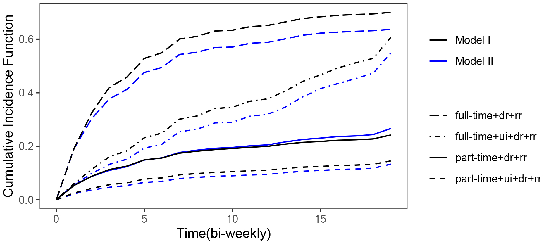
The cumulative incidence function estimates of exit to full-time and part-time employment with the effect of increasing dr via Model I & Model II.

McCall (1996) considered Unemployment Insurance (ui), Disregard rate (dr), Replacement Rate (rr) together with ui:dr and ui:rr to investigate the effect of increasing the dr on re-employment prospects for unemployed individuals. In the USA, the states allow individuals that are employed on part-time basis to continue to receive unemployment benefits provided their salaries do not exceed a certain amount (referred to as “disregard rate”). McCall (1996) contends that increasing the disregard rate will actually encourage unemployed individual to seek out part-time employment and overall improve employment. We also considered the same set of variables, and for ease of intepretation, we have centred dr and rr at their respective average values, and regard ui recipients, that is (ui $=$ 1) as the base. We found that the interaction terms were insignificant and we therefore excluded them. We fitted the proposed model (Model I) and a Complete Case version of the same model where the subjects with missing failure causes are excluded. We have referred to this model as Model II. It means that for Model II, the missingness indicator variable $m$ falls away and the model is reduced to an ordinary competing risks model that was proposed by Ndlovu et al. (2019). We have referred to full-time employment and part-time employment as failure type 1 & 2, respectively. We have chosen failure type 1 as our cause of interest and modelled the probability of failure due to this type of failure via a binomial model;

$\displaystyle\pi_{1}(\bm{x};\bm{\gamma}_{1})=\frac{\gamma_{01}+\exp(\bm{x}^{T}% \bm{\gamma}_{1})}{1+\gamma_{01}+\exp(\bm{x}^{T}\bm{\gamma}_{1})}$ (15)

Note that $\pi_{2}(\bm{x};\bm{\gamma}_{2})=1-\pi_{1}(\bm{x};\bm{\gamma}_{1})$ . The results of the analysis are displayed in Table 1. For illustrative purposes, we investigated the effect of increasing the disregard rate by 50% by assessing this effect on the cumulative incidence function. It can be seen from the Fig. 1 that according to both models that there is a noticeable drop in the full-time employment, but there is no significant movement in part-time employment. Model I suggests that there is a marginal decrease in part-time employment, whereas, Model II pionts towards marginal increase. The difference between Model I and Model II regarding part-time employment may be due to the fact that about 18% of data was discarded due to missing failure causes. Evidently, there is a move away from full-time to part-time employment according to both Model I & II, but there is no significant increase in part-time employment as claimed by McCall (1996). Possibly, the difference between our findings and the findings by McCall (1996) can be attributed to the differences in data sets used for analysis. Note that we could predict the direction of the movement in the cumulative incidence function by examining the parameter estimates. Since $\hat{\beta}_{1\textit{dr}}<0$ and $\hat{\gamma}_{1\textit{dr}}<0$ for Model I, it means that increasing the disregard rate, and holding other variables constant, will engender a reduction in the component hazards for exit to full-time employment and another drop in the marginal probability of exit to full-time employment, which ultimately translates to a reduction in $(1-\hat{S}(t|\bm{x};\hat{\bm{\beta}})\times\hat{\pi}_{1}(\bm{x};\hat{\bm{% \gamma}}))$ for ui recipients. On the other hand, there is a decrease in the component hazards for exit to part-time employment induced by $\hat{\beta}_{2\textit{dr}}<0$ as well. If the marginal probability of exit to full-time employment has dropped due to the increase in dr, the marginal probability to exit to part-time employment will increase because $\pi_{2}=(1-\pi_{1})$ . It is not possible to predict the cumulative effect of these movements in this instance with regards to the effect of increasing the disregard rate on exits to part-time employment. These predictions are only possible if the component hazards and the marginal failure type probabilities move in the same direction. For Model II, both the component hazards and the failure type probabilities drop for full-time employment which results in a reduction full-time employment. The component hazards drop whilst the failure type probabilities increase for part-time employment, as a result, the movement in the cumulative incidence function that is induced by an increase in dr cannot be predicted.

Figure 2.

The cumulative incidence function estimates of exit to full-time and part-time employment with the effect of ui via Model I & Model II.

We have also applied the proposed model to confirm the widely accepted theory in macroeconomics that, whilst unemployment benefits provide financial support to unemployed individuals they also have unintended consequence of increasing the unemployment rate, they act as a disincetive instead of encouraging unemployed individuals to intensify their efforts to search for employment. Recall that ui $=$ 1 is the base category, i.e., unemployment benefit recepients are regarded as the base group. Since $\hat{\beta}_{1\textit{ui}}>0$ and $\hat{\gamma}_{1\textit{ui}}<0$ , we cannot predict the effect of ui on the probability of full-time employment for non recepients, but we can predict the effect of ui on the probability of part-time employment, that is, the effect of ui is to increase the probability of part-time employment. This holds true in the absence or presence of missing failure causes. We have plotted the effect of ui on the cumulative incidence function in Fig. 2. The plot of cumulative incidence functions agrees with theory, that is, unemployment benefits do tend to act as a disincetive.

4. Conclusions

In this article we have developed a mixture regression model for analysis of competing risks data that has unknown failure causes for some of the subjects. The original continuous time model that was advanced by Larson and Dinse (1985) was upscaled as suggested by the authors to a missing failure causes model and modified for application in discrete time. We have demonstrated that the unknown parameters of the model can be estimated via the application of a multinomial distribution and a Poisson distribution. We have also demonstrated that the movement of the cumulative incidence functions can be predicted from the parameter estimates provided that the covariate effect induces the component hazards and the failure type probabilities to move in the same direction. It was demonstrated that the model can be applied to discrete time data with missing failure causes. The discrete time competing risks models are cause-specific-hazard denominated (Ambrogi et al., 2009; Tutz, 1995; Tutz & Schmid, 2016; Lee et al., 2018), i.e., they advance the cause-specific-hazards for modelling data. This means that all these models cannot be applied in the presence of missing failure causes. The proposed model, therefore, presents an option that can be considered when discrete time data comes with missing failure causes.

References

Ambrogi

Biganzoli

, & Boracchi

(2009). Estimating Crude Cumulative incidences through Multinomial Logit Regression on Discrete Cause Specific Hazard. Computational Statistics and Data Analysis, 53, 2767-2779.

Anderson

Goetghebeur

, & Ryan

(1996). Missing cause of death information in the analysis of survial data. Statistics in Medicine, 16, 2191-2201.

Begg

C.B.

, & Gray

(1984). Calculation of polytomous logistic regression parameters using individualized regressions. Biometrika, 71, 11-18.

Betancur

M.M.

(2013). Regression modeling with missing outcomes: competing risks and longitudinal data.PhD thesis, Universite Paris Sud.

Choi

(2002). On the Mixture Models in Survival Analysis with Competing Risks and Covariates. PhD thesis, Hong Kong polytechnic University.

Cox

(1972). Regression Models and Life Tables. Journal of Royal Statistical Society B, 34, 187-220.

Croissant

, & Graves

(2020). Ecdat: Data Sets for Econometrics. R package version 0.3-7.

Dewanji

(1992). A note on a test for competing risks with missing failure. Biometrica, 79, 855-857.

Dinse

G.E.

(1982). Nonparametric estimation for partially-complete time and of failure data. Biometrics, 38, 417-431.

10.

Escarala

, & Bowater

R.J.

(2008). FittiNG A SEMI-PARAMETRIC MIXTURE MODEL FOR COMPETING RISKS IN SURVIVAL Data. Communications in Statistics – Theory and Methods, 37, 277-293.

11.

Goetghebeur

, & Ryan

(1990). A modified logrank test for competing risks with missing failure type. Biometrika, 77, 207-211.

12.

Goetghebeur

, & Ryan

(1995). Analysis of competing risks survival data when some failure types are missing. Biometrika, 82, 821-834.

13.

Haller

(2014). The Analysis of Competing Risks Data with a Focus on Estimation of Cause-Specific and Subdistribution Hazard Ratios from a Mixture Model. PhD thesis, Ludwig-Maximiliäns-Universitat München.

14.

Holford

(1980). The Analysis of rates and of survivorship using log-linear models. Biometrics, 36, 299-305.

15.

Laird

, & Oliver

(1981). Covariance analysis of censored survival data using log-linear analysis techniques. Biometrica, 76, 231-240.

16.

Larson

M.G.

, & Dinse

G.E.

(1985). A mixture model for the regression analysis of competing risks data. Journal of the Royal Statistical Society. Series C (Applied Statistics), 34, 201-211.

17.

Lau

Cole

, & Gange

(2011). Parametric mixture models to evaluate and summarize hazard ratios in the presence of competing risks with time-dependent hazards and delayed entry. Statistic in Medicine, 30, 654-665.

18.

Lau

Cole

S.R.

Moore

R.D.

, & Gange

S.J.

(2008). Evaluating competing adverse and beneficial outcomes using a mixture model. Stat Med, 27, 4313-4313.

19.

Lee

Feuer

, & Fine

(2018). On the analysis of discrete time competing risks data. Biometrics. doi: 10.1111/biom.12881.

20.

, & Tsiatis

(2001). Multiple imputation methods for estimating regression coefficients in the competing risks model with missing cause of failure. Biometrics, 57, 1191-1197.

21.

Maller

, & Zhou

(2002). Analysis of parametric models for competing risks. Statistica Sinica, 12, 725-750.

22.

McCall

B.P.

(1996). Unemployment insurance rules, joblessness, and part-time work. Econometric Society, 64, 647-682.

23.

McLachlan

Yau

K.W.

, & Lee

(2004). Modelling the distribution of ischaemic stroke-specific survival time using an em-based mixture approach with random effects adjustment. Stat Med, 23, 2729-2744.

24.

S.K.

, & McLachan

G.J.

(2003). An EM-based semi-parametric mixture model approach to the regression analysis of competing-risks data. Stat Med, 22, 1097-1111.

25.

Nicolaie

van Houwelingen

H.C.

, & Putter

(2010). Vertical modeling: A pattern mixture approach for competing risks modeling. Statistics in Medicine, 29, 1190-1205.

26.

Nicolaie

M.A.

Taylor

, & Legrand

(2018). Vertical modeling: analysis of competing risks data with a cure fraction. Lifetime Data Analysis.

27.

Nicolaie

M.A.

van Houwelingen

H.C.

, & Putter

(2015). Vertical modelling: Analysis of competing risks data with missing causes of failure. Statistical Methods in Medicine, 29, 1190-1205.

28.

Peng

, & Taylor

(2014). Cure Models, chapter 6, pages 113–134. Chapman and Hall, Boca Raton, USA.

29.

Prentice

R.L.

Kalbfleisch

J.D.

Peterson

A.V.

Flournoy

Farewell

V.T.

, & Breslow

N.E.

(1978). The analysis of failure times in the presence of competing risks. Biometrics, 34, 541-554.

30.

Rubin

D.B.

(1976). Inference and missing data. Biometrika, 63, 581-592.

31.

Tutz

(1995). Competing risks models in discrete time with nominal or ordinal categories of response. Quality and Quantity, 29, 405-420.

32.

Tutz

, & Schmid

(2016). Modeling Discrete Time-to-Event Data. Springer.

33.

Zhiping

(2011). On Competing Risks data with covariates and Long-term Survivors. PhD thesis, Hong Kong Polytechnic University.

34.

Ndlovu

Melesse

, & Zewotir

(2019). A mixture model with application to discrete competing risks data. South African Journal of Statistics, 2, 73-86.

An EM model for analysis of discrete time competing risks data with missing failure causes

Abstract

Keywords

1. Introduction

Table 1 Maximum likelihood estimates (with standard errors) for Model I & II ( * denotes P < 0.05)

References

Table 1
Maximum likelihood estimates (with standard errors) for Model I & II ( ${}^{*}$ denotes $P<$ 0.05)