Non-compliance to Benford distribution as the portfolio default rate determinant in online retail lending

Abstract

There is large online lending growth in volume world-wide. The credit risk concerns point to the fact that most of these loans might be used to redeem earlier borrowed funds. However, the true reasons for online borrowing and lending are unavailable. Benford law is one of the tools used by auditors to monitor how suspicious the transaction is. That is why I wish to study one of the publicly available lending portfolios. Our objective is to trace associativity of compliance to Benford law and reported default rates. I find that MAE is a more statistically significant determinant of the country portfolio default rate, than RMSE. Moreover, the least creditworthy portfolios seem to be those with the MAE around 52–56%, while the closest to Benford and the least adjacent distribution do not demonstrate that large default rates.

Keywords

Peer-to-peer lending P2P default rate Mintos maturity LTV

1. Introduction

The online lending becomes an important domain to monitor as such lending might be used to merely refinance the existing borrowings. This may generate the negative contagion effect when the borrowers start to default. Such a non-natural (non-productive, speculative) motive to borrow online may change the observed data patterns. That is why I wish to study whether the alike abnormalities are related to the reported default rates in the domain of the online lending.

One of the tools to discover data abnormalities is the Benford (Newcomb-Benford) law. It is a stylized distribution often observed in real-life data, like the Zipf law. The difference is that the Zipf’s law corresponds to the distribution of entire values, while the Benford one focuses on the distribution of the first digits in these values. The Benford law is often used to trace the fraudulent nature in the financial data. However, the mere non-compliance to this law is not a fraud signal, unless the association with the fraudulent status is confirmed.

That is why our objective is to benchmark the available portfolio default data against the degree of compliance to Benford law. As a preview of our research findings, the key contribution is that Benford-compliance measures do not equivalently signal for the default rate. For instance, the mean absolute error (MAE) is more informative, than the root mean squared error (RMSE). Moreover, the larger the degree of non-compliance is, the default rate is not always higher. There is a break-even distance around MAE equal to 52–56%. This means that the least portfolio default rates are observed for the extreme compliance measures, i.e., for the smallest and for the largest. The worst default rate is associated with the non-extreme compliance to Benford. This implies that it is incorrect to treat non-compliance to Benford as a negative default rate determinant always.

To demonstrate the pathway to our findings I briefly cover the relevant literature in Section 2. I discuss the available data in Section 3. Then I describe our methodology in Section 4. Empirical findings are available in Section 5. Section 6 concludes the paper. Annex describes the data used in more detail.

2. Literature review

The Benford’s (Newcomb-Benford) law was discovered in the nineteenth century and formalized in the twentieth. Its idea is the parameterization of the probability density function $f_{X}(x)$ :

$\displaystyle f_{X}(x)=\log_{10}\left(1+\frac{1}{x}\right),$ (1)

where $f_{X}(x)$ is probability density function for the random variate $X$ in the point $x$ ; where $X$ is the random variate standing for the first digit in a sequence of figures; $x$ are its realizations varying from one to nine.

The Benford law is applied to various datasets. Hürlimann (2006) compiled a 15-page list of papers that dealt with it by 2006. There is a large stock of papers looking at the fraudulent nature of the financial data via the Benford lens (see Nigrini (2012), Nigrini (2017), Gomes da Silva and Carreira (2013)). Benford law application to the election data is covered in Lipovetsky (2021); Anderson et al. (2022), while Moreau investigates the COVID-19 statistics Moreau (2021). Our paper is closer to the first group as processes the credit registry data.

However, some authors mention the recommendation that the dataset should possess certain features prior to Benford law application. (Anderson et al., 2022, p. 841) state that “ $\ldots$ data sets that are spread out over several orders of magnitude are often close to Benford”. Singleton (2011) formulates this as “Benford’s Law holds true for a data set that grows exponentially (e.g., doubles, then doubles again in the same time span), but also appears to hold true for many cases in which an exponential growth pattern is not obvious”.

Nevertheless, even not meeting this recommendation does not prevent one from applying the Benford law. If it occurs useful and non-compliance to Benford has implications to the outcome variable of interest (e.g., in fraud detection), then one can proceed with applying it. For instance, Nigrini (2017) does not request such conditions to hold prior to inspecting the financial transactions.

Singleton (2011) adds that sometimes the Benford law application is useful when the process has a threshold. For instance, if there is a committee decision required at transactions above certain amount, the individual might wish undertaking all the deals at right below the threshold amount. Then it might be useful to look at the distribution of the first two digits. In case there is a data clustering, Anderson et al. (2022) suggest looking at the Benford law modification to the base of 3 (and not 10 as conventionally used).

There is a separate stream of literature with the generalization of Benford law Kossovsky (2014), Fang and Chen (2020) and the probable modifications to the distance metrics when measuring compliance with it da Silva et al. (2020). As no one processed Mintos data using the Benford law, I start with the baseline measures like MAE and RMSE presented in Eqs (2) and (3).

$\displaystyle\textit{MAE}=\frac{1}{9}\cdot\sum_{x=1}^{9}|f_{X}(x)-h_{X}(x)|,$ (2)

where $f_{X}(x)$ is the canonical Benford law density distribution from Eq. (1); and $h_{X}(x)$ is the empirical distribution density of the first digits $x$ ranging from one to nine.

$\displaystyle\textit{RMSE}=\frac{1}{9}\cdot\sum_{x=1}^{9}(f_{X}(x)-h_{X}(x))^{% 2}.$ (3)

For the reader’s information, Cerqueti and Maggi (2021) propose to refer to the first measure as a mean absolute deviation (MAD), rather than MAE following (Nigrini, 2012, p. 160). They also propose to focus on the sum of squared deviations (SSD), rather than RMSE in accordance to Kossovsky (2014).

The publications by the central bankers devoted to the use of the Benford’s law gave us idea to apply the law to the novel dataset. For instance, Croatian and Finnish central bankers discovered that the financials of the failed banks demonstrated violation to Benford’s law in Krakar and Žgela (2009); Kauko (2019), respectively. While Krakar and Žgela (2009) focused on the foreign-currency nominated loans of the Croatian banks; Kauko (2019) investigated non-performing loans’ figures in Chinese banks. Similar patterns were found for banks in the United States by Alalia and Romero (2013); Grammatikos and Papanikolaou (2021), for Turkey by Uzuner (2014), and in Russia by Davydov and Swidler (2016).

3. Data evidence

I depart from the European peer-to-peer (P2P) lending platform Mintos being inspired by the works of Nigmonov for it Nigmonov (2021) and for its US counterpart, the Lending Club Nigmonov et al. (2022). Figure 1 presents the loan portfolio accumulation by the loan issue date. The data specifics is that it is a sort of a portfolio snapshot and not a time series of defaults. For instance, the observed hike in default rate in 2018–2019 means that those are defaults of loans originated in these years and probably securitized via Mintos. However, it is not that evident when the default triggered.

Figure 1.

Mintos reported loan book volume and default rate.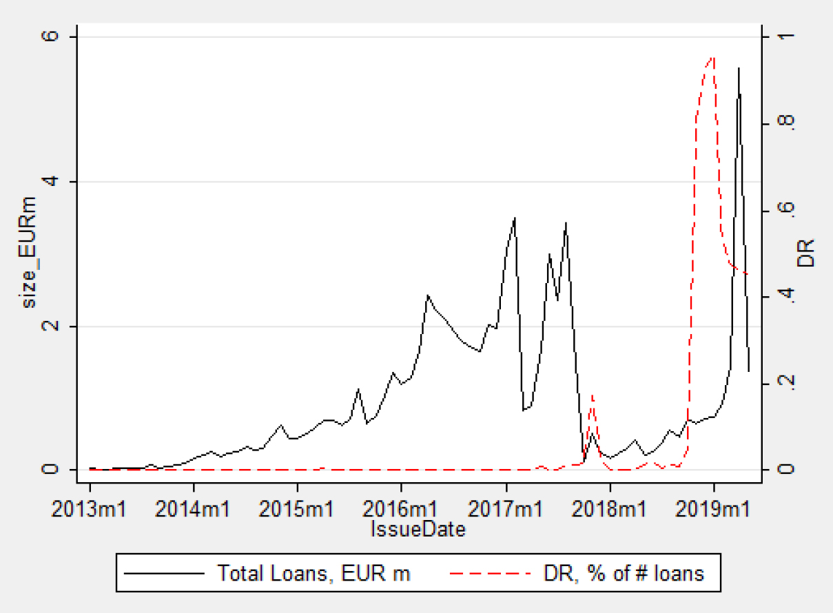

There are the key facts about this publicly available dataset below:

•

The Mintos portfolio was downloaded by the author after free of charge registration on the website from https://www.mintos.com/en/loan-book/download on July 10, 2021;

•

The loan portfolio volume in a zip-archive is 2.7 Gb;

•

It consists of 71 csv-files (6.2 Gb without archive), each containing 500 k entries. Thus, the entire book seems to comport 35 m (35 432 467) loans.

The data specifics forced developing a loop-algorithm to process each of the 71 files separately and then merge the aggregate statistics to a single one. Otherwise, the standard Stata license fails to process such a volume of data.

I proceed with the following variables available from the Mintos loan portfolio data:

•

DR – Default Rate, proportion;

•

MAE – Mean absolute error, proportion, see Eq. (2);

•

MAE sq – Squared MAE value;

•

RMSE – Root mean squared error, proportion, see Eq. (3);

•

RMSE sq – Squared RMSE value;

•

Amount EUR – Initial loan amount in EUR k, conversion rate as of Jul. 10, 2021;

•

Maturity – The loan maturity in years, difference between issue and close dates;

•

Initial LTV – Initial loan-to-value, proportion;

•

Collateral – The flag for the collateral presence, mean proportion when aggregated;

Two outlier definitions were applied at the aggregate “country-loan type” level:

•

Abnormally high initial LTV (above 4.5, or 450%) – excluded 1 observation out of 1182;

•

Abnormally high loan amount (above EUR 50 k; only two of them are reported as mortgages) – excluded 8 observations out of 1182.

Annex has the descriptive statistics of the variables used (see Table 4) and pairwise correlations after filtering for outliers (see Table 5).

Initial loan amounts are considered in local currencies and extract the first digits from these amounts. Let us first verify where our dataset meets the desired criteria of doubling and whether it spreads over several orders of magnitude. The right column in Table 1 evidences the so-called doubling of the observed values by the listed percentiles as recommended by Singleton (2011).

Table 1

Initial loan amount in local currencies

Percentile	Value	Ratio to the above percentile value
Min	3.41
1	13.32	3.9
5	24.59	1.8
10	37.30	1.5
25	70.82	1.9
50	141.38	2.0
75	294.82	2.1
90	681.12	2.3
95	1768.42	2.6
99	15 k	8.5
Max	25 m	1666.7

Note: k – thousands; m – millions.

Figure 2 shows that the data spreads over several orders of magnitude. The initial loan amount in local currency ranges from 3.41 to 25 m with its natural logarithm ranging from 1.2 to 17.0. Breaking down the data by loan types still preserves the feature of spreading over several orders of magnitude, see Fig. 3. There is neither a threshold for data collection (except the one from the bottom in the invoice financing).

Figure 2.

The distribution of the logarithm of loan amounts in national currencies in the pooled dataset spreads over several orders of magnitude.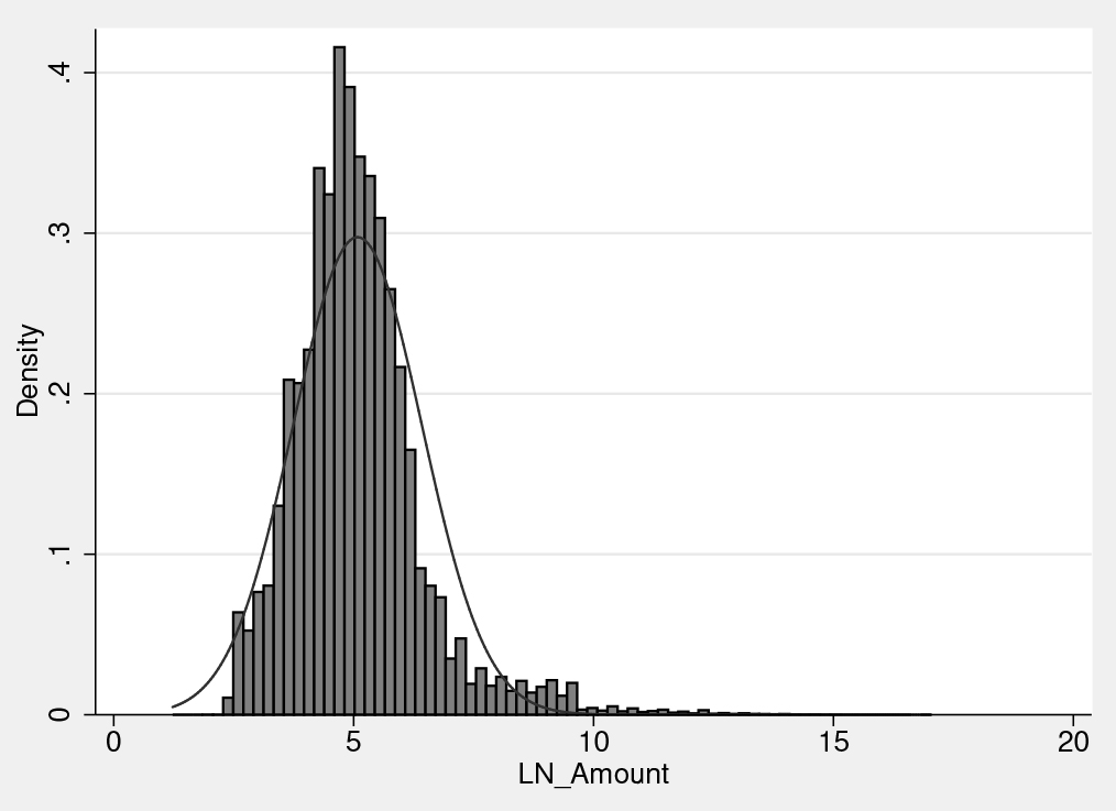

Figure 3.

The distribution of the logarithm of loan amounts in national currencies per loan types evidences for the presence of clustered data in Business loans (2), pawnbroking loans (7). Cut-off floor might be typical for Invoice financing loans (5). Note: 1 – Agricultural; 2 – Business; 3 – Car; 4 – Forward Flow; 5 – Invoice Fin.; 6 – Mortgage; 7 – Pawnbroking; 8 – Personal; 9 – Short-Term.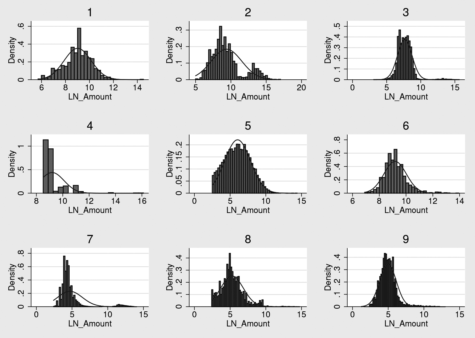

Thus, the available Mintos dataset was “naturally” collected and it meets the recommendation with respect to cases when the Benford law is applicable.

The highest-level view on the data brings evidence of its overall compliance to Benford law, except for mortgages, see Fig. 4. The distance measure varies by loan type when break-downing the dataset to more granular levels. Pawnbroking loans (seem to be just a different name to the personal and short-term (ST) loans) seems to be quite common in initial loan amounts from the Benford law perspective, see Fig. 5. However, at least, for the processed dataset Mintos does not report any defaults for mortgages, cars or pawnbroking loans.

Figure 4.

Mintos-wide the first digit distribution seems to be benford-compliant, except for mortgages.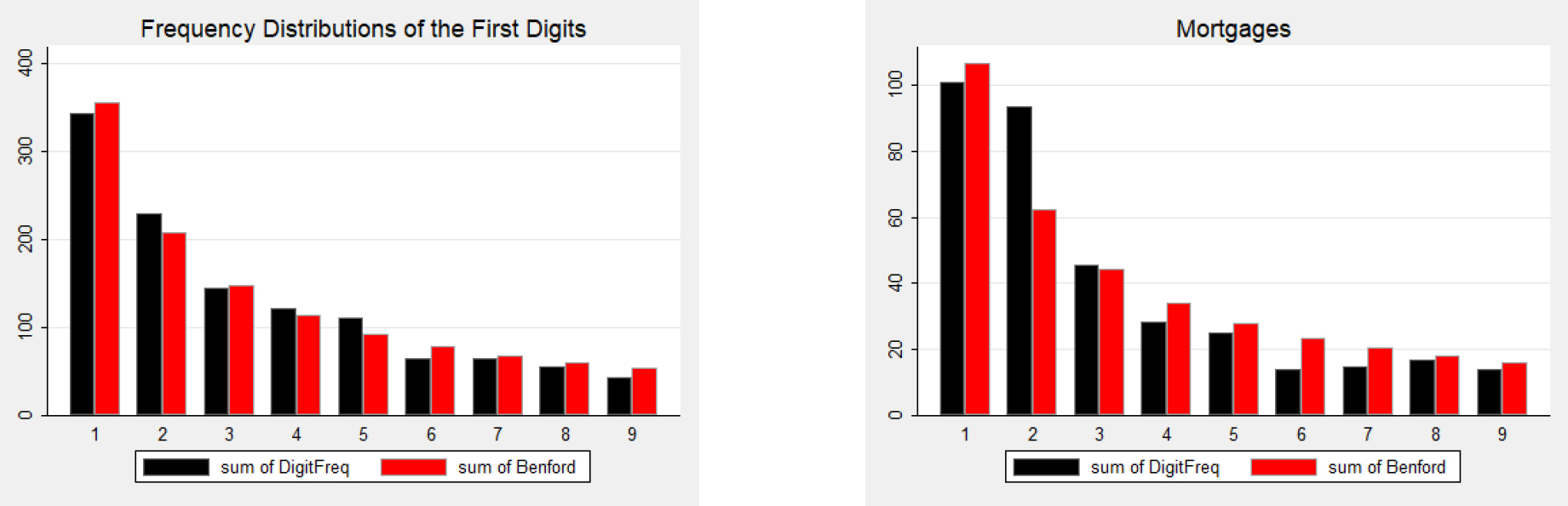

Figure 5.

RMSE demonstrates more variability, than MAE in Mintos data.

Historically it can be seen that the initial loan amounts become more compliant with the Benford law, see Fig. 6. However, this is in part an effect of the growing loan portfolio by number of loans. Interestingly, the Russian subportfolio had a sharp rise in non-compliance degree after the oil shock of 2016. Nevertheless, Mintos reports zero default rates for the Russian portfolio.

Figure 6.

MAE tend to decrease faster in time, than RMSE (left – entire sample; right – Russia).

Prior to running a multifactor analysis, I start from the visual pairwise scatterplot of the default rate and the Benford compliance measures (MAE, RMSE). Here I follow the example of Bank of Japan Bank of Japan (2019) when the default drivers were benchmarked against the default rate and not the single-loan default status. I define a default status if the “In recovery” variable has positive response (‘Yes’). The default rate (DR) is bimodally distributed with quite rare occasion of being different from zero or one. For instance, all loans in Zambia are reported to be in default. The scatterplots of MAE and RMSE against the default rate show that the linear and quadratic trends lie close to each other. However, when focusing on the quadratic ones only, there might be a break-even point. Before reaching that point in error terms the default rate rises and falls afterwards. The effect is more pronounced for the ‘other’ category of loans, see Fig. 7.

Figure 7.

For the ‘other’ loan types the quadratic dependence of the default rate and the distance measure is more pronounced.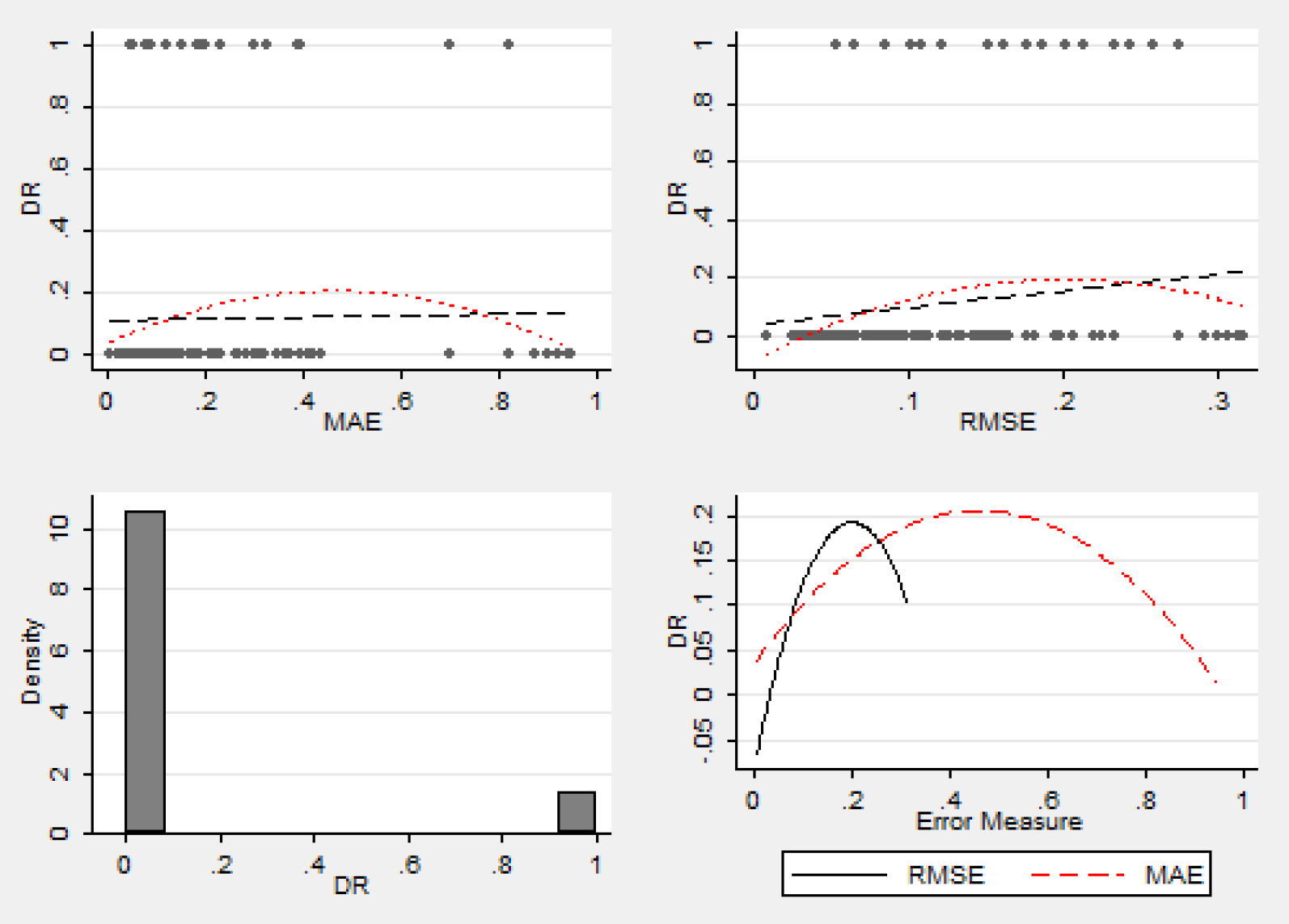

The wide-spread credit risk (default rate) determinants – the loan size, maturity, loan-to-value, collateral – demonstrate semi-conventional (or semi-expected) patterns in the data, see Fig,. 8.

Figure 8.

The available factors tend to be negatively associated with the portfolio default rate.

The mean trends are negative in association with the default rate. As for the loan size, the larger amounts are borrower by larger – hence more reliable – borrowers. The larger the maturity is, the lower the default rate is. This contradicts to the logic of the Internal Ratings-Based (IRB) approach prescribed by the Basel Committee BCBS (2019). The committee thinks that the longer the loan maturity is, the more uncertainty about the success to redeem it is BCBS (2005). However, it well corresponds to the observation by the Nobel laureate in economics Robert Merton. He argues that the longer the horizon is, the more chances the borrower has to find out alternative source to redeem the loan if the major source evaporates Merton (1974). The more collateral is offered, the less the default rate is. This may seem natural. However, the larger the initial loan-to-value (LTV) is – i.e., the riskier the borrower seems to be – the lower the default rate is. Moreover, the collateral presence is positively correlated with the initial LTV. It is strange as more collateral seems to deliver a signal of a creditworthy borrower, while the more initial LTV is, the signal is right the opposite – the borrower is less creditworthy. This signals that the reported data may be biased in the unknown direction to us. That is why one should be cautious further on in interpreting our findings.

4. Modeling methodology

I implement the following regression specification to benchmark the default rate against the distance measure and its squared value:

$\displaystyle\textit{DR}_{ijt}=\theta_{1}\cdot\textit{Dist}_{ijt}+\theta_{2}% \cdot\textit{Dist}_{ijt}^{2}+\beta_{1}\cdot\textit{EUR}_{ijt}+\beta_{2}\cdot% \textit{LTV}_{ijt}+\beta_{3}\cdot M_{ijt}+\beta_{4}\cdot\textit{Col}_{ijt}+% \epsilon_{ijt},$ (4)

where $\textit{DR}_{ijt}$ is the default rate for the i-th country j-th loan type at the $t$ -th issue date; $\textit{Dist}_{ijt}$ is the degree of compliance to Benford law (distance). It is MAE or RMSE. $\textit{EUR}_{ijt}$ is the initial loan amount in thousands of EUR for the respective ijt-th bucket, $\textit{LTV}_{ijt}$ is the loan-to-value; $M_{ijt}$ – loan maturity; $\textit{Col}_{ijt}$ – the proportion of collateral solicited by the lender; $\epsilon_{ijt}$ is the noise term; $\theta$ and $\beta$ are the coefficients subject to estimation by ordinary least squares. Annex with Tables 4 and 5 has more information on the descriptive statistics of the variables employed and their pair-wise correlations.

5. Empirical findings

I try running the regression over the entire sample (pool) and for the subset with non-zero default rates (DRpos). The latter set excludes car, pawnbrowking loans and mortgages. I run separate regressions for short-term (ST) and personal loans, as well as for the other ones. Table 2 reports the repression output for the MAE distance measure and Table 3 – for RMSE.

Table 2
Default rate determinants: compliance benford distribution via MAE

Variable	m pool	m ST	m Pers	m oth	m DRpos
MAE	0.25**	0.15	0.14	1.02***	0.17
MAE sq	$-$ 0.28**	$-$ 0.38	$-$ 0.19	$-$ 1.05***	$-$ 0.24
Amount EUR	0	$-$ 0.47***	$-$ 0.06	0	$-$ 0.09**
Maturity	0	$-$ 0.39	0.01	0.03	0.01
Initial LTV	$-$ 0.01	(omitted)	(omitted)	$-$ 0.05	0.1
Collateral	$-$ 0.12***	(omitted)	(omitted)	$-$ 0.32***	$-$ 0.22
cons	0.11***	0.28***	0.12***	0.08	0.14***
N obs.	1173	160	393	154	577
R2	7.0%	7.0%	0.0%	16.0%	1.0%
R2 adj	6.0%	5.0%	-1.0%	13.0%	0.0%

Note: Statistical significance at *** 1%, ** 5%, * 10%.

Table 3

Default rate determinants: compliance benford distribution via RMSE

Variable	r pool	r ST	r Pers	r oth	r DRpos
RMSE	0.48	1.64	$-$ 0.34	4.12***	0.07
RMSE sq	$-$ 1.32	$-$ 6.8	0.58	$-$ 10.23***	$-$ 0.71
Amount EUR	0	$-$ 0.47***	$-$ 0.05	0	$-$ 0.09**
Maturity	0	$-$ 0.41	0.01	0.01	0.01
Initial LTV	$-$ 0.01	(omitted)	(omitted)	$-$ 0.02	0.1
Collateral	$-$ 0.12***	(omitted)	(omitted)	$-$ 0.35***	$-$ 0.22
cons	0.10***	0.21*	0.15***	$-$ 0.07	0.15***
N obs.	1173	160	393	154	577
R2	6.0%	7.0%	0.0%	20.0%	1.0%
R2 adj	6.0%	5.0%	-1.0%	16.0%	0.0%

Note: Statistical significance at *** 1%, ** 5%, * 10%.

Table 4

Descriptive statistics of the variables used in the study

Variable	Mean	Std. Dev.	Min	Max
DR	0.07	0.25	0.00	1.00
MAE	0.19	0.25	0.01	0.95
MAE sq	0.10	0.23	0.00	0.91
RMSE	0.11	0.08	0.01	0.32
RMSE sq	0.02	0.02	0.00	0.10
Amount EUR	3.84	6.19	0.05	46.24
Maturity	2.49	2.22	0.04	17.84
Initial LTV	0.31	0.39	0.00	2.33
Collateral	0.43	0.48	0.00	1.00

Note: the total number of observations for each variable equals to 1173.

Table 5

Correlation matrix of the variables used

	DR	MAE	MAE sq	RMSE	RMSE sq	Amount	Maturity	Initial LTV
MAE	$-$ 0.03
MAE sq	$-$ 0.04	0.97
RMSE	0.00	0.94	0.87
RMSE sq	$-$ 0.01	0.97	0.95	0.97
Amount EUR	$-$ 0.05	0.21	0.16	0.19	0.17
Maturity	$-$ 0.14	0.31	0.28	0.27	0.27	0.24
Initial LTV	$-$ 0.23	0.04	0.02	0.02	0.02	0.22	0.42
Collateral	$-$ 0.25	0.10	0.08	0.07	0.07	0.28	0.53	0.90

I find a meaningful association of the two Benford compliance degrees and the default rate for other loans and only that of MAE for the pooled dataset. The findings are significant at 5% level. Moreover, I find that the squared Benford compliance degree values also matter. Using the rule for the parabola extreme, the break-even points for the pooled dataset and other loans in terms of MAE. It is 52 and 56%. These values correspond to the highest default rates, while full compliance and material non-compliance turn out to be bearable from the credit risk perspective.

As for other default rate determinants, I find significantly negative coefficients for the loan size and collateral presence. The controversial indicators of maturity and initial LTV occur to be non-significant.

The overall model fit is not high. R-squared adjusted reaches its peak of 13% and 16% for other loans only, being negative for the personal ones. When putting our research objective, I wished to check what association can be traced from the available data. I am the first to evidence that it is overall low, though Benford-compliance metrics might matter for the entire sample and for the other loans. Though MAE and RMSE in general are close to each other, I was able to reveal differences when applied to particular loan category.

6. Conclusions

Online lending attracts more and more attention nowadays in the developed Nigmonov et al. (2022) and well as in the developing economies Selmier II (2017). Benford law is known for two centuries and is actively used by auditors of the financial statements Nigrini (2017). However, no one previously inspected the online lending data with respect to its compliance with the Benford law. Our research closes this gap. To do this a special loop-code in Stata was prepared to be able to process the large volume of the Mintos portfolio data.

I contribute by making two statements:

•

The mean absolute error (MAE) is a more significant determinant of the portfolio default rate, than the root mean squared error (RMSE). This corresponds to the choice of this measure as the reference statistical distance for Benford law compliance by Cerqueti and Maggi in Cerqueti and Maggi (2021).

•

The large non-compliance to Benford should not be for granted considered as the indicator of the future defaults, at least in the available Mintos dataset. There is a break-even point of around 52–56% in terms of MAE. Before this point increase in the degree of Benford non-compliance is associated with the rise in the default rate; but after bypassing it the default rate decreases.

Though our findings are novel, one should be cautious in its extrapolation for several reasons:

•

I revealed an inconsistency in the initial LTV values. This may signal that the data is poorly registered or there might be some other data specifics not yet disclosed to us.

•

The portfolio data has to explicit default date for the defaulted loans. Thus, I am unable to link it to the known material macroeconomic events for at least a sort of robustness check.

•

The reported data has strange outliers and features. Some countries like Russia demonstrate no defaults. By probability theory and given large number of loans in this subset, there should be defaults unless there is some particular unreported bias in loan choice. Same time China having the largest loans in size has no reasonable explanation.

Footnotes

Acknowledgments

Author is grateful to Alexander Shapoval and other participants of the Modeling and Analysis of Complex Systems and Processes (MACSPro) conference in December 2021. Author acknowledges feedback from Mario Maggi for the first draft of the paper and to Stan Lipovetsky for discussions about the paper and the Benford law application in general. Author is grateful to anonymous reviewer for useful comments.

Disclaimer

The views expressed in this paper are solely those of the author and do not necessarily reflect the official position of the affiliated institutions. The Bank of Russia assumes no responsibility for the contents of the paper.

References

Alalia

, & Romero

(2013). Characteristics of failed U.S. commercial banks: an exploratory study. Accounting and Finance, 53, 1149-1174. doi: 10.1111/j.1467-629X.2012.00491.x, restricted access.

Anderson

K. M.

Dayaratha

Gonshorowski

, & Miller

S. J.

(2022). A new Benford test for clustered data with applications to American elections. MDPI Stats, 5, 841-855. doi: 10.3390/stats5030049, free access.

Bank of Japan (2019). A Forecast Model for the Probability of Default Based on Granular Firm-Level Data and Its Application to Stress Testing.

BCBS (2005). An explanatory note on the Basel II IRB risk weight functions. http://www.bis.org/bcbs/irbriskweight.htm.

BCBS (2019). CRE – calculation of RWA for credit risk. https://www.bis.org/basel_framework/standard/CRE.htm.

Cerqueti

, & Maggi

(2021). Data validity and statistical conformity with Benford’s Law. Chaos, Solitons and Fractals, 144, 110740.

da Silva

Floquet

Santos

, & Lima

(2020). On the validation of the Newcomb – Benford Law and the Weibull distribution in neuromuscular transmission. Physica A, 553.

Davydov

, & Swidler

(2016). Reading Russian tea leaves: Assessing the quality of bank financial statements with the Benford distribution. Review of Pacific Basin Financial Markets and Policies, 19, 1650021.

Fang

, & Chen

(2020). Several common probability distributions obey Benfordâ€™s law. Physica A, 540.

10.

Gomes da Silva

, & Carreira

(2013). Selecting audit samples using Benfordâ€™s Law. Auditing: A Journal of Practice & Theory, 32(2), 53-65.

11.

Grammatikos

, & Papanikolaou

N. I.

(2021). Applying Benford’s law to detect accounting data manipulation in the banking industry. Journal of Financial Services Research, 59, 115-142. https://link-springer-com-443.web.bisu.edu.cn/content/pdf/10.1007/s10693-020-00334-9.pdf, free access.

12.

Hürlimann

(2006). Benford’s law from 1881 to 2006. https://www.researchgate.net/publication/2129354_Benford’s_law_from_1881_to_2006. free access; accessed on December 11, 2022.

13.

Kauko

(2019). Benford’s law and Chinese banksâ€™ non-performing loans. https://helda.helsinki.fi/bof/bitstream/handle/123456789/16533/dp2519.pdf. BOFIT Discussion Papers No. 25; free access; accessed 14 August 2022.

14.

Kossovsky

(2014). Benford’s Law: Theory, the General Law of Relative Quantities, and Forensic Fraud Detection Applications. World Scientific Pub.

15.

Krakar

, & Žgela

(2009). Application of Benford’s law in payment systems auditing. https://www.researchgate.net/publi-cation/26630504_Application_of_Benford%27s_Law_in_Payment_Systems_Auditing. Free access.

16.

Lipovetsky

(2021). Understanding Elections Through Statistics: Polling, Prediction, and Testing. Technometrics, 63(1), 143-144.

17.

Merton

(1974). On the pricing of corporate debt: The risk structure of interest. Journal of Finance, 29, 449-470.

18.

Moreau

V. H.

(2021). Inconsistencies in countries COVID-19 data revealed by Benford’s law. Model Assisted Statistics and Applications, 16(1), 73-79.

19.

Nigmonov

(2021). Banking versus fintech credit: Estimating defaults in European P2P lending market. presentation at the annual event of finance research letters. 2021 virtual conference: Frontiers in credit risk.

20.

Nigmonov

Shams

, & Alam

(2022). Macroeconomic determinants of loan defaults: Evidence from the U.S. peer-to-peer lending market. Research in International Business and Finance, 59, 101516.

21.

Nigrini

M. J.

(2012). Benfordâ€™s Law: Applications for Forensic Accounting, Auditing, and Fraud Detection. John Wiley and Sons, New York.

22.

Nigrini

M. J.

(2017). Audit sampling using benfordâ€™s law: A review of the literature with some new perspectives. Journal of Emerging Technologies in Accounting, 14(2), 29-46.

23.

Selmier II

W. T.

(2017). Folk Lending and P2P: Monitoring Maturation in Chinese Financial Contracting. The China Business Model, pp. 169-193.

24.

Singleton

T. W.

(2011). Understanding and applying Benfordâ€™s law. https://www.isaca.org/resources/isaca-journal/past-issues/2011/understanding-and-applying-benfords-law. free access; accessed on December 11, 2022.

25.

Uzuner

(2014). sApplication of Benford’s law to the traded consolidated balance sheets of banks in Istanbul stock exchange. Finansal Araştırmalar ve Çalışmalar Dergisi, 19, 1650021. https://dergipark.org.tr/en/pub/marufacd/issue/507/4598, restricted access.