Development of out-of-sample forecast formulae for the FIGARCH model

Abstract

Volatility is a matter of concern for time series modeling. It provides valuable insights into the fluctuation and stability of concerning variables over time. Volatility patterns in historical data can provide valuable information for predicting future behaviour. Nonlinear time series models such as the autoregressive conditional heteroscedastic (ARCH) and the generalized version of the ARCH model, i.e. generalized ARCH (GARCH) models are popularly used for capturing the volatility of a time series. The realization of any time series may have significant statistical dependencies on its distant counterpart. This phenomenon is known as the long memory process. Long memory structure can also be present in volatility. Fractionally integrated volatility models such as the fractionally integrated GARCH (FIGARCH) model can be used to capture the long memory in volatility. In this paper, we derived the out-of-sample forecast formulae along with the forecast error variances for the AR (1) -FIGARCH (1, $d$ , 1) model by recursive use of conditional expectations and conditional variances. For empirical illustration, the modal spot prices of onion for Delhi, Lasalgaon and Bengaluru markets, India and S&P 500 index (close) data are used.

Keywords

Long memory nonlinear time series models GARCH volatility

1. Introduction

The autoregressive integrated moving average (ARIMA) model paved the way for the development of time series modeling (Box and Jenkins, 1970). The ARIMA methodology is structured based on the assumption of linearity and homoscedasticity of prediction error variances. In reality, many time series data sets did not adhere to these assumptions due to the presence of volatility. Engle (1982) proposed the autoregressive conditional heteroscedastic (ARCH) model to capture the time-varying volatility observed in financial returns. Bollerslev (1986) and Taylor (1986) independent of each other, proposed the generalized ARCH (GARCH) model. Later the fractional integration term has been incorporated into the GARCH model to capture the long memory and it is termed as the fractionally integrated GARCH (FIGARCH) model (Baillie et al., 1996).

Agricultural commodities exhibit volatility in their prices. The possible causes of price volatility may be the shocks due to the sudden disruption in the supply chain (Paul and Birthal, 2021; Paul and Yeasin, 2022; Ruan et al., 2021) or natural phenomena such as rainfall, flood, drought, pest and disease attack, etc. The volatility study of agricultural time series can be found in the literature (Gurung et al., 2017; Mitra and Paul, 2017; Anjoy and Paul, 2019; Paul and Garai, 2021; Paul and Karak, 2022; Rakshit et al., 2023). Again, the prices of agricultural commodities can have long term persistence in the mean model (Mitra and Paul, 2021; Paul et al., 2021; Paul et al., 2022), in the variance model (Paul et al., 2016; Rakshit and Paul, 2023) or both (Mitra et al. 2018).

In modeling, the in-sample forecasts are obtained and compared with the observations in the model validation set to measure the efficacy of the selected model. The out-of-sample forecasting of future observations can be done by using the naïve approach. In this approach, at first, a one-step-ahead forecast is done. This realization is considered as the original observation and included in the model building set. Again, the parameters are re-estimated to forecast for its next one-step-ahead forecast. In this step-by-step process, a multi-step ahead forecast is executed. No direct forecasting formula is available in the literature for multi-step ahead forecasts for fractionally integrated variance models like the FIGARCH model. In this research paper, we derived the formulae for out-of-sample forecast and forecast error variances for the AR(1)- FIGARCH (1, $d$ , 1) model by recursive use of conditional expectations and conditional variances in the same line of Ghosh et al. (2010). For empirical illustration, the modal spot prices of onion for Delhi, Lasalgaon and Bengaluru markets, India and S&P 500 index (close) data are used. The price volatility of onion price in India is a matter of concern for researchers (Paul et al., 2015; Birthal et al., 2019; Saxena et al., 2019; Das et al., 2020; Saxena et al., 2020; Rakshit et al., 2021). The volatility study of the S&P 500 index is a prime topic throughout the world (Mason and Elkassabgi, 2022; Qu and He, 2022; Zhang et al., 2022; Garai and Paul, 2023; Mudiangombe and Muteba Mwamba, 2023). This paper is organized as follows: Section 2 includes a brief description of the ARCH and GARCH models, the FIGARCH model along with the derivation of out-of-sample forecast formulae and forecast error variances of the AR(1)- FIGARCH (1, $d$ , 1) model; Section 3 is the results and discussion where empirical illustrations are given followed by concluding remarks in Section 4.

2. Materials and methods

2.1 The ARCH/GARCH model

The ARCH model is designed to address the heteroscedasticity present in any time series, where volatility tends to cluster over certain periods. The key idea behind the ARCH model is that the conditional variance of a time series is related to its past squared residuals or shocks. The ARCH model assumes that shocks of the time series have a direct impact on the volatility, creating a feedback mechanism. If the past squared residuals have a significant impact on the current conditional variance, it suggests the presence of ARCH effects.

Let $\left\{{\varepsilon_{t}}\right\}$ be a process and the available information up to $t-1$ time period is $\psi_{t-1}$ . Then the conditional distribution of $\left\{{\varepsilon_{t}}\right\}$ given $\psi_{t-1}$ is said to follow the ARCH ( $q$ ) if it is represented as:

$\displaystyle\varepsilon_{t}|\psi_{t-1}\sim N\left({0,h_{t}}\right)\ \text{and% }\ \varepsilon_{t}=\sqrt{h_{t}}\nu_{t}$ (1)

where $\nu_{t}$ is identically and independently distributed (IID) with zero mean and unit variance. This is known as innovation.

The conditional variance $h_{t}$ of ARCH ( $q$ ) model is calculated as

$\displaystyle h_{t}=\alpha_{0}+\mathop{\sum}\limits_{i=1}^{q}\alpha_{i}% \varepsilon_{t-i}^{2},\alpha_{0}>0,\alpha_{i}\geqslant 0\ \forall i\ \ \text{% and}\ \mathop{\sum}\limits_{i=1}^{q}\alpha_{i}<1$ (2)

An extension of the ARCH model is the GARCH model, which incorporates both lagged squared residuals and lagged conditional variances in the model equation. The GARCH model is a more parsimonious model than the ARCH model. The GARCH ( $p, q$ ) process has the following form of conditional variance

$\displaystyle h_{t}=\alpha_{0}+\mathop{\sum}\limits_{i=1}^{q}\alpha_{i}% \varepsilon_{t-i}^{2}+\mathop{\sum}\limits_{j=1}^{p}\beta_{j}h_{t-j}$ $\displaystyle\text{provided}\ \alpha_{0}>0,\alpha_{i}\geqslant 0\ \forall i,\ % \beta_{j}\geqslant 0\ \forall j$ (3)

$\alpha_{i}$ and $\beta_{j}$ are the measures of how the current volatility is affected by earlier shocks and volatilities respectively. The GARCH ( $p, q$ ) process is said to be weakly stationary if and only if

$\displaystyle\mathop{\sum}\limits_{i=1}^{q}\alpha_{i}+\mathop{\sum}\limits_{j=% 1}^{p}\beta_{j}<1$ (4)

2.2 The FIGARCH model

The FIGARCH model allows for the estimation of the long memory parameter present in the conditional variance, which indicates the degree of persistence in volatility over time. A detailed review of the FIGARCH model can be found in Tayefi and Ramanathan (2012).

The conditional variance equation of GARCH ( $p, q$ ) is given by

$\displaystyle h_{t}=\alpha_{0}+\mathop{\sum}\limits_{i=1}^{q}\alpha_{i}% \varepsilon_{t-i}^{2}+\mathop{\sum}\limits_{j=1}^{p}\beta_{j}h_{t-j}$ (5)

This representation can also be expressed as an equivalent ARMA type representation as

$\displaystyle\varepsilon_{t}^{2}=\alpha_{0}+\mathop{\sum}\limits_{i=1}^{q}% \alpha_{i}\varepsilon_{t-i}^{2}+\mathop{\sum}\limits_{j=1}^{p}\beta_{j}% \varepsilon_{t-j}^{2}-\mathop{\sum}\limits_{j=1}^{p}\beta_{j}z_{t-j}+z_{t}$ (6)

where $z_{t}=\varepsilon_{t}^{2}-h_{t}=h_{t}v_{t}^{2}-h_{t}=\left({v_{t}^{2}-1}\right% )h_{t}$

This equation can be expressed as an ARMA ( $m, p$ ) process in $\varepsilon_{t}^{2}$ as

$\displaystyle\left[{1-\alpha\left(L\right)-\beta\left(L\right)}\right]% \varepsilon_{t}^{2}=\alpha_{0}+\left[{1-\beta\left(L\right)}\right]z_{t}$ (7)

where, $m=\max\left\{{p,q}\right\}$ , $\beta\left(L\right)$ and $\alpha\left(L\right)$ are polynomials in the lag operator. This $\left\{{z_{t}}\right\}$ process can be regarded as the innovations for the conditional variance. From this ARMA ( $m, p$ ) process equation, the integrated GARCH ( $p, q$ ) process is defined as

$\displaystyle\left[{1-\alpha\left(L\right)-\beta\left(L\right)}\right]\left({1% -L}\right)\varepsilon_{t}^{2}=\alpha_{0}+\left[{1-\beta\left(L\right)}\right]z% _{t}$ (8)

From this integrated GARCH process the FIGARCH models can be obtained by taking the fractional differencing operator $\left({1-L}\right)^{d}$ instead of the first difference operator $\left({1-L}\right)$ in (Eq. (8)), where $d$ is a fraction $0<d<1$ . Here, the long memory operator is applied to the squared errors. Hence, the FIGARCH $\left({p,d,q}\right)$ model can be expressed as

$\displaystyle\left[{1-\alpha\left(L\right)-\beta\left(L\right)}\right]\left({1% -L}\right)^{d}\varepsilon_{t}^{2}=\alpha_{0}+\left[{1-\beta\left(L\right)}% \right]z_{t}$ (9)

For any value of the differencing parameter $d$ , the term $\left({1-L}\right)^{d}$ can be extended as

$\displaystyle\left({1-L}\right)^{d}=1-dL+\frac{L^{2}d\left({d-1}\right)}{2!}+% \ldots=\mathop{\sum}\limits_{j=0}^{\infty}\left({{\begin{array}[]{*{20}c}d% \hfill\\ j\hfill\\ \end{array}}}\right)\left({-1}\right)^{j}L^{j}$ (10)

where,

$\displaystyle\left({{\begin{array}[]{*{20}c}d\hfill\\ j\hfill\\ \end{array}}}\right)=\frac{d!}{j!\left({d-j}\right)!}=\frac{\Gamma\left({d+1}% \right)}{\Gamma\left({j+1}\right)\Gamma\left({d-j+1}\right)}$ (11)

and $\Gamma\left(.\right)$ is the gamma function.

2.3 Out-of-sample forecast formulae for AR (1) – FIGARCH (1,

d

, 1) model

In the context of modeling, a common practice is to divide the available dataset into two subsets: the model building set and the model validation set. The model building set is used to develop and estimate the parameters of the model.

Suppose, $T$ data points are used for model building and $k$ data points are used for validation purposes for a time series dataset.

Let the mean model AR (1) be fitted on the time series data as the linear model. Hence,

$\displaystyle y_{T}=\mu+\phi_{1}y_{T-1}+\varepsilon_{T}$ (12)

where, $\varepsilon_{T}|\psi_{T-1}\sim N\left({0,h_{T}}\right)$ and $\varepsilon_{t}=\sqrt{h_{T}}\nu_{T}$

$\psi_{T-1}$ is the information available up to $T-1$ time period. And $\nu_{T}$ is independently and identically distributed (IID) innovation with zero mean and unit variance.

Lemma 1: The i^th -step ahead out-of-sample forecast obtained by recursive use of conditional expectation is

$\displaystyle\hat{y}_{T+k+i}=\hat{\mu}\sum^{i-1}_{j=0}\hat{\phi}^{j}_{1}+\hat{% \phi}^{i}_{1}y_{T+k}$ (13)

(the proof is given in Appendix 1).

2.4 Forecast error variance for AR (1) – FIGARCH (1,

d

, 1) model

Lemma 2: The i^th -step ahead forecast error variance obtained by recursive use of conditional expectations and conditional variances is

$\displaystyle\sigma_{T+k+i|1,2,\ldots,T+k}^{2}=E\left(\hat{h}_{T+k+i}\right)=% \hat{\alpha}_{0}+\hat{\beta}_{1}\sigma^{2}+(\hat{\alpha}_{1}+\hat{d})\left[% \hat{\alpha}_{0}\left\{\sum^{i-3}_{j=0}(\hat{\alpha}_{1}+\hat{\beta}_{1}+\hat{% d})^{j}\right\}+(\hat{\alpha}_{1}+\hat{\beta}_{1}+\hat{d})^{i-2}\hat{h}_{T+k+1% }\right]$ (14)

(the proof is given in Appendix 2).

3. Results and discussion

The daily time series data for the modal spot prices (Rs./q) of onions for the markets in Delhi, Lasalgaon, and Bengaluru from 1^st January 2008 to 30^th June 2022 are obtained from the Ministry of Agriculture & Farmers’ Welfare, Government of India. S&P 500 index data (close) for the same period are also obtained from the website of Yahoo Finance. For the daily price series, the total number of observations is 5295 and for the S&P 500 index, it is 3650. All the analysis is done based on the log return series of the daily data series since the square of return is regarded as the realization of volatility. Another advantage of using the return series is that it dismisses the presence of seasonal effects. The log return series $\left\{{r_{t}}\right\}$ for a financial time series $\left\{{y_{t}}\right\}$ is calculated as

$\displaystyle r_{t}=\ln\frac{y_{t}}{y_{t-1}}$ (15)

The reason behind taking the daily series is that the daily series over a long period has a large number of realizations which has a greater possibility to show long term persistence in volatility. The log return series of the selected time series are divided into two parts, the last 250 realizations are considered the model validation set and the remaining previous portion as the model building set.

Table 1

Descriptive statistics of selected onion price series and S&P 500 index (close)

Statistics	Delhi	Lasalgaon	Bengaluru	S&P 500
Mean (Rs./q)	1354.22	1326.33	1364.87	2166.53
Median (Rs./q)	1064.00	990.00	1036.67	2020.11
Minimum (Rs./q)	275.00	230.50	300.00	676.53
Maximum (Rs./q)	7650.00	8625.00	12500.00	4796.56
S.D. (Rs./q)	909.47	1048.37	1069.44	993.33
C.V. (%)	67.16	79.04	78.36	45.85
Skewness	2.07	2.07	3.31	0.82
Kurtosis	5.42	5.52	19.23	$-$ 0.11

Figure 1.

Time plot of the selected time series, onion price series of (a) Delhi, (b) Lasalgaon, (c) Bengaluru markets, and (d) S&P 500 index (close).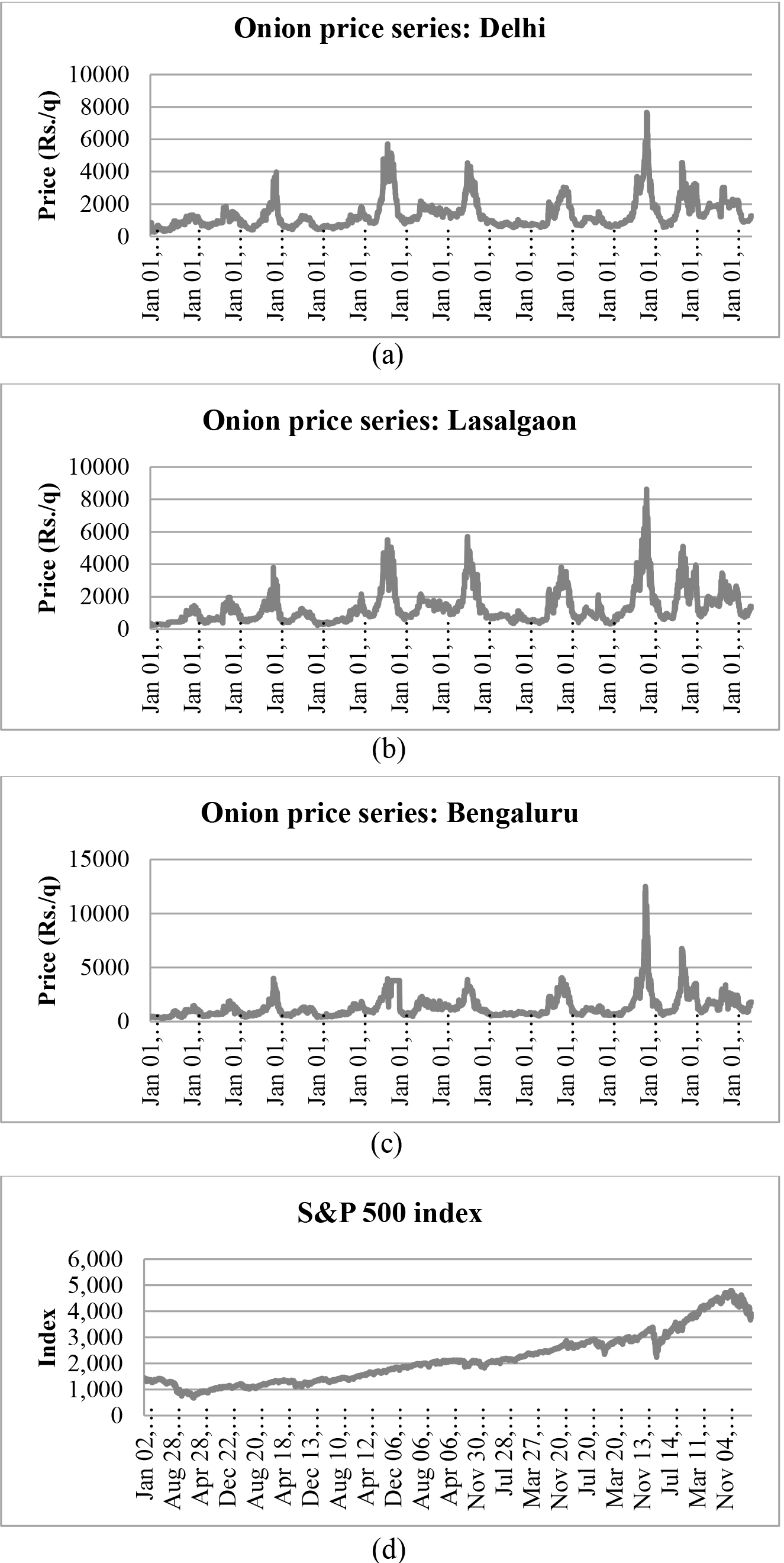

The descriptive statistics of the selected time series are given in Table 1. A relatively high level of C. V. percentage can be seen for all the price series. The S&P 500 index has a relatively lower C. V. percentage than them. The selected price series are more positively skewed than the S&P 500 index. All the price series are leptokurtic and the Bengaluru market price series exhibits a high degree of leptokurtosis. But, the S&P 500 index is platykurtic. The time plot of the selected series is given in Fig. 1. From Fig. 1, it can be seen that all three onion price series follow a similar pattern. The price rise and fall occurred at the very same time for all three markets. The S&P 500 index has two major downfalls during the study period, one during the 2008 financial crisis and another one during the 2020 COVID-19 pandemic.

Table 2

Test for stationarity of the selected series

Log return
Test	Delhi	Lasalgaon	Bengaluru	S&P 500
ADF	$-$ 17.47^***	$-$ 16.30^***	$-$ 16.43^***	$-$ 15.23^***
PP	$-$ 82.45^***	$-$ 82.04^***	$-$ 78.60^***	$-$ 69.43^***
Squared log return
ADF	$-$ 14.57^***	$-$ 16.16^***	$-$ 16.03^***	$-$ 8.62^***
PP	$-$ 65.32^***	$-$ 61.74^***	$-$ 71.16^***	$-$ 51.13^***

${}^{***}p\leqslant$ 0.01.

Stationarity is a fundamental assumption in time series analysis and modeling. Stationarity is often a requirement for estimating time series models accurately. Non-stationary data can lead to biased parameter estimates, unreliable model diagnostics, and incorrect inferences. The stationarity of the log return series and the squared log return series of the selected series are tested (Table 2) using the Augmented Dickey-Fuller (ADF) test (Dickey and Fuller, 1979) and Phillips-Perron (PP) test (Phillips and Perron, 1988). The null hypothesis for both tests is that the unit root is present in the time series. It is seen that both tests are significant for all the selected series and the null hypothesis has been rejected. As the selected log return series are stationary, the AR model can be fitted directly without any differentiation.

Figure 2.

The ACF plots for the squared log return series of (a) Delhi, (b) Lasalgaon, (c) Bengaluru markets, and (d) S&P 500 index (close).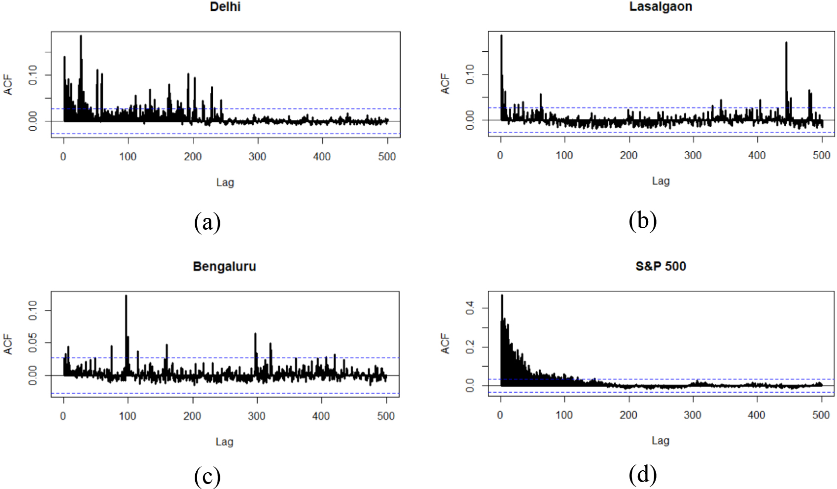

Long term persistence of a time series is a phenomenon which arises when there is significant statistical dependence among the realizations of the process occurring at distant lags. Long memory can exist both in linear and nonlinear dynamics of the time series data. The autocorrelation function (ACF) and partial autocorrelation function (PACF) plots are commonly used as a visualizing tool for indicating the statistical dependencies and relationships among the successive realizations of a time series. If long term persistence among the realizations is present then, the autocorrelation function (ACF) decays slowly (hyperbolic decay). Otherwise, ACF decays at a much faster rate (exponential decay). For the instance of long memory in volatility, the ACF of the squared return series has hyperbolic decay. From the ACF and PACF plots of the log return series of the selected series, it is revealed that significant statistical dependencies are present among the successive observations. Again, these ACF and PACF plots exhibited exponential decay. The ACF plots of the corresponding squared series for up to 500 lag are given in Fig. 2((a)–(d)). The dotted line indicates the confidence interval at a 95% significance level. From the ACF plots of the squared log return series, it can be seen that significant autocorrelation is present among the distant realizations. This indicates the presence of the long memory phenomenon in the variance model. This is very much prominent for the ACF plots of the squared log return series of Delhi’s onion price series and the S&P 500 index.

Table 3

The GPH test: Test for long memory

	Delhi		Lasalgaon		Bengaluru		S&P 500
	Log return	Squared log return	Log return	Squared log return	Log return	Squared log return	Log return	Squared log return
$d$	$-$ 0.05	0.30	$-$ 0.02	0.06	$-$ 0.04	0.09	0.08	0.30
S.D.	0.06	0.06	0.06	0.03	0.05	0.04	0.08	0.08
Z	$-$ 0.86	5.29	$-$ 0.38	2.32	$-$ 0.71	2.06	0.96	3.60

Table 4

Parameter estimates of the fitted AR(1)- FIGARCH (1, $d$ , 1) model

Parameters	Delhi	Lasalgaon	Bengaluru	S&P 500
Mean model
Constant	$-$ 0.00 (0.00)	0.00 (0.00)^*	0.00 (0.00)	0.00 (0.00)^***
AR(1)	$-$ 0.02 (0.02)	$-$ 0.09 (0.02)^***	$-$ 0.06 (0.02)^***	$-$ 0.07 (0.02)^***
Variance model
Constant	0.00 (0.00)^***	0.00 (0.00)^***	0.00 (0.00)^***	0.00 (0.00)^***
$\alpha_{1}$	0.39 (0.01)^***	0.38 (0.02)^***	0.36 (0.04)^***	0.02 (0.04)
$\beta_{1}$	0.63 (0.01)^***	0.70 (0.02)^***	0.46 (0.04)^***	0.50 (0.06)^***
$d$	0.33 (0.01)^***	0.46 (0.02)^***	0.15 (0.01)^***	0.62 (0.04)^***

^***p < 0.01, ^**p < 0.05, ^{* p <} 0.10; S.E. is in parenthesis.

After visualizing the presence of long memory in volatility, it is tested by the GPH test (Geweke & Porter-Hudak, 1983). From Table 3 it can be seen that for the selected log return series the estimates of the fractional differencing parameters are not significant. However, for the squared log return series, the estimates of the fractional differencing parameters are significant. It suggests that all the squared log return series contain a long memory structure. Hence, the presence of long term persistence in the volatility is confirmed. This result supports the inferences drawn from the ACF and PACF plots.

Table 5

In-sample forecasting performance in the model validation set for the selected return series

Series	Model	RMSE	MAE
Delhi	ARMA (1,0) -FIGARCH (1, $d$ , 1)	0.04	0.01
Lasalgaon	ARMA (1,0) -FIGARCH (1, $d$ , 1)	0.07	0.04
Bengaluru	ARMA (1,0) -FIGARCH (1, $d$ , 1)	0.09	0.05
S&P 500	ARMA (1,0) -FIGARCH (1, $d$ , 1)	0.01	0.01

As the log return series of the selected time series are stationary, the AR(1) model is fitted as the mean model to each of them in the model building set. After fitting the AR(1) model, the residuals are calculated and the ARCH-LM test is used to evaluate the presence of conditional heteroscedasticity. The null hypothesis for the ARCH-LM test is the absence of the ARCH effect in the residual series. For each of the empirical cases, the test is significant. Once the presence of conditional heteroscedasticity is confirmed, the FIGARCH (1, $d$ , 1) model is fitted to each residual series. The estimates of the parameters are given in Table 4. The parameters are estimated using the maximum likelihood estimation process. It is seen that almost all the parameters are significant at a 1% level of significance. The ARCH parameter $\alpha_{1}$ is not significant for the S&P 500. It indicates that for the S&P 500, the current volatility is not significantly affected by previous shocks. The fractional differencing parameter $d$ is significant for each scenario and is within its permissible range. The adequacy of the fitted model is ensured by examining the residuals and it is found that all the residual series are white noise. The in-sample forecasting performance of the fitted AR(1)- FIGARCH (1, $d$ , 1) model is evaluated using two error functions namely Root Mean Squared Error (RMSE) and Mean Absolute Error (MAE) in the model validation set. These two error functions are calculated as

$\displaystyle\textit{RMSE }=\left[{\frac{1}{k}\mathop{\sum}\limits_{t=1}^{k}% \left({r_{t}-\hat{r}_{t}}\right)^{2}}\right]^{1/2}$ (16)

$\displaystyle\textit{MAE}=\frac{1}{k}\mathop{\sum}\limits_{t=1}^{k}\left|{r_{t% }-\hat{r}_{t}}\right|$ (17)

where $k$ is the number of horizons used for validation, $r_{t}$ is the observed return and $\hat{r}_{t}$ is the corresponding predicted return. The calculated values of these error functions are given in Table 5.

Table 6

Out-of-sample forecast of the return series along with forecast error variance

Series (log return)	Horizon	Forecast	Forecast error variance
Delhi	1	$-$ 0.0004	0.0008
	2	$-$ 0.0004	0.0030
	3	$-$ 0.0004	0.0034
Lasalgaon	1	0.0044	0.0026
	2	0.0009	0.0069
	3	0.0013	0.0082
Bengaluru	1	0.0003	0.0035
	2	0.0003	0.0053
	3	0.0003	0.0058
S&P 500	1	0.0014	0.0002
	2	0.0007	0.0002
	3	0.0007	0.0002

The out-of-sample forecast for the next three horizons from the derived formula of the AR (1) -FIGARCH (1, $d$ , 1) model along with the forecast error variance is given in Table 6 for the selected return series. Crucial decisions can not be taken only based on the future forecasted values. Some degree of risk is always associated with forecasted values. This risk increases along the length of the forecast horizon. Forecast error variance is the realization of that risk. For the Delhi and Bengaluru markets, the forecasts for the next three horizons are almost the same and due to rounding off upto four decimals, they became the same. For Lasalgaon, all three forecasts are different. For the S&P 500, the two-step ahead and three-step ahead forecasts are the same due to rounding off. It is seen that the forecast error variances are increasing with the increase of forecast horizons for all the selected time series. For the S&P 500 index, due to rounding off decimal numbers, they are the same. From the derived formula of the forecast error variance, it can also be seen that it increases as the horizon of the forecast increases. Hence, it is better to forecast for a short period.

4. Conclusions

In this paper, we derived the out-of-sample forecast formulae and the forecast error variance for the AR (1) -FIGARCH (1, $d$ , 1) model by recursive use of conditional expectations and conditional variances. For empirical illustration purposes, the log return series of four time series namely modal spot prices of onion in Delhi, Lasalgaon and Bengaluru of India and the S&P 500 series are used. All the selected time series exhibit the presence of long memory in volatility. The derived formulae for out-of-sample forecast using the FIGACRH model have been applied and the forecast of these series along with the forecast error variances have been obtained. The forecasted values for a shorter horizon are more reliable. It is advisable to forecast for a shorter horizon as the forecast error variance increases with the increase of the forecasting horizon. The unexpected fluctuation of the price of agricultural commodities is a concerning matter to all the stakeholders in the supply chain from farmers to consumers as well as the policymakers. A prior knowledge of price volatility can help farmers to sell their produce profitably. Government agencies can also take preventive measures to stop unexpected price falls. Hence, proper knowledge of volatility is extremely important for efficient planning and monitoring of the agricultural production system. From the modeling point of view, this research work can be extended to the other fractionally integrated variance models.

Footnotes

Acknowledgments

The authors are thankful to the Director, ICAR-IASRI; the Joint Director (Education) & Dean, The Graduate School, ICAR-IARI and the Director, ICAR-IARI for providing the required research facilities.

Appendix 1

The one-step-ahead out-of-sample forecast is given by

(18) $\displaystyle\hat{y}_{T+k+1}=\hat{y}_{T+k+1|1,2,\ldots,T+k}=E\left({y_{T+k+1}|% y_{1},y_{2},\ldots,y_{T+k}}\right)=\hat{\mu}+\hat{\phi}_{1}y_{T+k}$

Similarly, the two-step ahead out-of-sample forecast is derived by recursive use of conditional expectation as

(19) $\displaystyle\hat{y}_{T+K+2}=\hat{y}_{T+k+2|1,2,\ldots,T+k}=E(y_{T+k+2}|y_{1},% y_{2},\ldots,y_{T+k})=E\left(\hat{y}_{T+k+2|1,2,\ldots,T+k+1}|y_{1},y_{2},% \ldots,y_{T+k}\right)=\hat{\mu}+\hat{\phi}_{1}\hat{y}_{T+k+1}=\hat{\mu}+\hat{% \phi}_{1}(\hat{\mu}+\hat{\phi}y_{T+k})=\hat{\mu}(1+\hat{\phi}_{1})+\hat{\phi}_% {1}^{2}y_{T+k}$

Similarly, the three-step ahead out-of-sample forecast can be derived as

(20) $\displaystyle\hat{y}_{T+k+3}=\hat{\mu}+\hat{\mu}\hat{\phi}_{1}+\hat{\mu}\hat{% \phi}^{2}_{1}+\hat{\phi}^{3}_{1}y_{T+k}$

Going forward this way, the i^th-step ahead out-of-sample forecast can be obtained by recursive use of conditional expectation as

(21) $\displaystyle\hat{y}_{T+k+i}=\hat{\mu}\sum^{i-1}_{j=0}\hat{\phi}^{j}_{1}+\hat{% \phi}^{i}_{1}y_{T+k}$

Appendix 2

To estimate the forecast error variance, let $\varepsilon_{T}$ follows a FIGARCH (1, $d$ , 1) process.

The conditional variance $h_{T}$ of the FIGARCH model is defined as follows,

$\displaystyle\left[{1-\beta\left(L\right)}\right]h_{T}=\alpha_{0}+\left[{1-% \beta\left(L\right)-\left({1-\alpha\left(L\right)-\beta\left(L\right)}\right)% \left({1-L}\right)^{d}}\right]\varepsilon_{t}^{2}$

Hence, the conditional variance $h_{T}$ of the FIGARCH (1, $d$ , 1) model is defined as:

$\displaystyle\left[{1-\beta_{1}L}\right]h_{T}=\alpha_{0}+\left[{1-\beta_{1}L-% \left({1-\alpha_{1}L-\beta_{1}L}\right)\left({1-L}\right)^{d}}\right]% \varepsilon_{t}^{2}$ $\displaystyle\Rightarrow h_{T}=\alpha_{0}+\beta_{1}h_{T-1}+\left[{1-\beta_{1}L% -\left({1-\alpha_{1}L-\beta_{1}L}\right)\left({1-dL}\right)}\right]\varepsilon% _{t}^{2}$

(taking up to the first order of approximation for the binomial expansion $\left({1-L}\right)^{d})$

(22) $\displaystyle\Rightarrow h_{T}=\alpha_{0}+\beta_{1}h_{T-1}+\left({\alpha_{1}+d% }\right)\varepsilon_{t-1}^{2}$

For the fitted model AR (1)-FIGARCH (1, $d$ , 1), the one-step-ahead out-of-sample forecast error variance is

(23) $\displaystyle\sigma_{T+k+1|1,2,\ldots,T+k}^{2}=E\left[{\left\{{y_{T+k+1}-\hat{% y}_{T+k+1|1,2,\ldots,T+k}}\right\}}^{2}|y_{1},y_{2},\ldots,y_{T+k}\right]=E% \left[{\varepsilon_{T+k+1|1,2,\ldots,T+k}^{2}}\right]=\hat{h}_{T+k+1}=\hat{% \alpha}_{0}+\hat{\beta}_{1}\hat{h}_{T+k}+(\hat{\alpha}_{1}+\hat{d})\hat{% \varepsilon}^{2}_{T+k}$

Again, the two-step ahead out-of-sample forecast error variance is

(24) $\displaystyle\sigma_{T+k+2|1,2,\ldots,T+k}^{2}=E\left[{\left\{{y_{T+k+2}-\hat{% y}_{T+k+2|1,2,\ldots,T+k}}\right\}}^{2}|y_{1},y_{2},\ldots,y_{T+k}\right]=E% \left[{E\left\{{y_{T+k+2}-\hat{y}_{T+k+2|1,2,\ldots,T+k+1}}\right\}}^{2}|y_{1}% ,y_{2},\ldots,y_{T+k}\right]+V\left[\hat{y}_{T+k+2|1,2,\ldots,T+k+1}|y_{1},y_{% 2},\ldots,y_{T+k}\right]=E\left[{E\left\{{\varepsilon_{T+k+2|1,2,\ldots,T+k}^{% 2}}\right\}}\right]+V\left(\hat{y}_{T+k+2}\right)=E(\hat{h}_{T+k+2})+V\left(% \hat{y}_{T+k+2}\right)$ (25) $\displaystyle=E\left(\hat{h}_{T+k+2}\right)+V\left[\hat{\mu}+\hat{\phi}_{1}% \hat{y}_{T+k+1}\right]=E\left(\hat{h}_{T+k+2}\right)+\hat{\phi}^{2}_{1}V(\hat{% y}_{T+k+1})$

Now,

$\displaystyle E(\hat{h}_{T+k+2})=E\left[\hat{\alpha}_{0}+\hat{\beta}_{1}\hat{h% }_{T+k+1}+(\hat{\alpha}_{1}+\hat{d})\hat{\varepsilon}_{T+k+1}^{2}\right]$

Now, as per the assumption

$\displaystyle\hat{\varepsilon}_{T+k+1}\sim N(0,\hat{h}_{T+k+1})$ $\displaystyle\Rightarrow E\left(\hat{\varepsilon}_{T+k+1}\right)=0\ \text{and}% \ V(\hat{\varepsilon}_{T+k+1})=E(\hat{\varepsilon}_{T+k+1}^{2})=\hat{h}_{T+k+1% }\ \text{and}\ E(\hat{h}_{T+k+1})=\sigma^{2}$

Hence,

$\displaystyle\sigma_{T+k+2|1,2,\ldots,T+k}^{2}=E(\hat{h}_{T+k+2})+\hat{\phi}_{% 1}^{2}V(\hat{y}_{T+k+1})=\hat{\alpha}_{0}+\hat{\beta}_{1}\sigma^{2}+(\hat{% \alpha}_{1}+\hat{d})\hat{h}_{T+k+1}+\hat{\phi}_{1}^{2}\hat{h}_{T+k+1}=\hat{% \alpha}_{0}+\hat{\beta}_{1}\sigma^{2}+(\hat{\alpha}_{1}+\hat{d}+\hat{\phi}_{1}% ^{2})\hat{h}_{T+k+1}\ \text{(from Eq.∼{}(\ref{eq22a}))}$

For $i\geqslant$ 3,

$\displaystyle\sigma_{T+k+i|1,2,\ldots,T+k}^{2}=E\left(\hat{h}_{T+k+i}\right)+V% (\hat{y}_{T+k+i})\ \text{(from Eq.∼{}(\ref{eq22}))}$

Here, $V\left(\hat{y}_{T+k+i}\right)$ contains large integer powers of $\hat{\phi}_{1}$ subsequently, which is too small as $\left|\hat{\phi}_{1}\right|\leqslant$ 1. Hence, we proceed further as

(26) $\displaystyle\sigma_{T+k+i|1,2,\ldots,T+k}^{2}=E\left(\hat{h}_{T+k+i}\right)$

After taking the expectations, expanding the conditional variance term and replacing the square residuals $\hat{\varepsilon}_{T+k+i}^{2}$ with their expected values $\hat{h}_{T+k+i}$ ,

(27) $\displaystyle\sigma_{T+k+3|1,2,\ldots,T+k}^{2}=\hat{\alpha}_{0}+\hat{\beta}_{1% }\sigma^{2}+(\hat{\alpha}_{1}+\hat{d})[\hat{\alpha}_{0}+(\hat{\alpha}_{1}+\hat% {\beta}_{1}+\hat{d})\hat{h}_{T+k+1}]$

and similarly,

(28) $\displaystyle\sigma_{T+k+4|1,2,\ldots,T+k}^{2}=\hat{\alpha}_{0}+\hat{\beta}_{1% }\sigma^{2}+(\hat{\alpha}_{1}+\hat{d})[\hat{\alpha}_{0}+\hat{\alpha}_{0}(\hat{% \alpha}_{1}+\hat{\beta}_{1}+\hat{d})+(\hat{\alpha}_{1}+\hat{\beta}_{1}+\hat{d}% )^{2}\hat{h}_{T+k+1}]$

Hence, it can be generalized as

(29) $\displaystyle\sigma_{T+k+i|1,2,\ldots,T+k}^{2}=E\left(\hat{h}_{T+k+i}\right)=% \hat{\alpha}_{0}+\hat{\beta}_{1}\sigma^{2}+(\hat{\alpha}_{1}+\hat{d})\left[% \hat{\alpha}_{0}\left\{\sum_{j=0}^{i-3}(\hat{\alpha}_{1}+\hat{\beta}_{1}+\hat{% d})^{j}\right\}+(\hat{\alpha}_{1}+\hat{\beta}_{1}+\hat{d})^{i-2}\hat{h}_{T+k+1% }\right]$

References

Anjoy

, & Paul

R. K.

(2019). Comparative performance of wavelet-based neural network approaches. Neural Computing and Applications, 31, 3443-3453.

Baillie

R. T.

Bollerslev

, & Mikkelsen

H. O.

(1996). Fractionally integrated generalized autoregressive conditional heteroskedasticity. Journal of Econometrics, 74(1), 3-30.

Birthal

Negi

, & Joshi

P. K.

(2019). Understanding causes of volatility in onion prices in India. Journal of Agribusiness in Developing and Emerging Economies, 9(3), 255-275.

Bollerslev

. (1986). Generalized autoregressive conditional heteroskedasticity. Journal of Econometrics, 31(3), 307-327.

Box

G. E. P.

, & Jenkins

(1970). Time Series Analysis, Forecasting and Control, Holden-Day: San Francisco, CA, USA.

Das

Paul

R. K.

Bhar

L. M.

, & Paul

A. K.

(2020). Application of Machine Learning Techniques with GARCH Model for Forecasting Volatility in Agricultural Commodity Prices. Journal of the Indian Society of Agricultural Statistics, 74(3), 187-194.

Dickey

D. A.

, & Fuller

W. A.

(1979). Distribution of the Estimators for Autoregressive Time Series with a Unit Root. Journal of the American Statistical Association, 74, 427-431.

Engle

R. F.

(1982). Autoregressive Conditional Heteroscedasticity with Estimates of the Variance of United Kingdom Inflation. Econometrica, 50(4), 987-1007.

Garai

, & Paul

R. K.

(2023). Development of MCS based-ensemble models using CEEMDAN decomposition and machine intelligence. Intelligent Systems with Applications, 18, 200202.

10.

Geweke

, & Porter-Hudak

(1983). The estimation and application of long memory time series models. Journal of Time Series Analysis, 4(4), 221-238.

11.

Ghosh

Paul

R. K.

, & Prajneshu . (2010). Nonlinear time series modeling and forecasting for periodic and ARCH effects. Journal of Statistics Theory and Practice, 4(1), 27-44.

12.

Gurung

Singh

K. N.

Paul

R. K.

Panwar

Gurung

, & Lepcha

(2017). An alternative method for forecasting price volatility by combining models. Communications in Statistics-Simulation and Computation, 46(6), 4627-4636.

13.

Mason

A. N.

, & Elkassabgi

(2022). Evidence of Abnormal Trading on COVID-19 Pfizer Vaccine Development Information. Journal of Risk and Financial Management, 15(7), 299.

14.

Mitra

, & Paul

R. K.

(2017). Hybrid time-series models for forecasting agricultural commodity prices. Model Assisted Statistics and Applications, 12(3), 255-264.

15.

Mitra

Paul

R. K.

, & Paul

A. K.

(2018). Statistical modelling for forecasting volatility in potato prices using ARFIMA-FIGARCH model. Indian Journal of Agricultural Sciences, 88(2), 268-272.

16.

Mitra

, & Paul

R. K.

(2021). Forecasting of Price of Rice in India Using Long-Memory Time-Series Model. National Academy Science Letters, 44(4), 289-293.

17.

Mudiangombe

B. M.

, & Muteba Mwamba

J. W.

(2023). Impacts of U.S. Stock Market Crash on South African Top Sector Indices, Volatility, and Market Linkages: Evidence of Copula-Based BEKK-GARCH Models. International Journal of Financial Studies, 11(2), 77.

18.

Paul

R. K.

, & Birthal

P. S.

(2021). The prices of perishable food commodities in India: the impact of the lockdown. Agricultural Economics Research Review, 34(2), 151-164.

19.

Paul

R. K.

, & Garai

(2021). Performance comparison of wavelets-based machine learning technique for forecasting agricultural commodity prices. Soft Computing, 25(20), 12857-12873.

20.

Paul

R. K.

Gurung

Paul

A. K.

, & Samanta

(2016). Long memory in conditional variance. Journal of the Indian Society of Agricultural Statistics, 70(3), 243-254.

21.

Paul

R. K.

, & Karak

(2022). Asymmetric Price Transmission: A Case of Wheat in India. Agriculture, 12(3), 410.

22.

Paul

R. K.

Mitra

Roy

H. S.

Paul

, & Yeasin

(2022). Forecasting price of Indian mustard (Brassica juncea) using long memory time series model incorporating exogenous variable. Indian Journal of Agricultural Sciences, 92(7), 825-30.

23.

Paul

R. K.

Sarkar

, & Yadav

S. K.

(2021). Wavelet based long memory model for modelling wheat price in India. Indian Journal of Agricultural Sciences, 91(2), 227-231.

24.

Paul

R. K.

Saxena

Chaurasia

, & Rana

(2015). Examining export volatility, structural breaks in price volatility and linkages between domestic and export prices of onion in India. Agricultural Economics Research Review, 28, 101-116.

25.

Paul

R. K.

, & Yeasin

(2022). COVID-19 and prices of pulses in Major markets of India: Impact of nationwide lockdown. Plos One, 17(8), e0272999.

26.

Phillips

P. C. B.

, & Perron

(1988). Testing for a unit root in time series regression. Biometrika, 75(2), 335-346.

27.

, & He

(2022). Predicting Volatility Based on Interval Regression Models. Journal of Risk and Financial Management, 15(12), 564.

28.

Rakshit

Paul

R. K.

, & Panwar

(2021). Asymmetric Price Volatility of Onion in India. Indian Journal of Agricultural Economics, 76(2), 245-260.

29.

Rakshit

Paul

R. K.

Yeasin

Emam

Tashkandy

, & Chesneau

(2023). Modeling Asymmetric Volatility: A News Impact Curve Approach. Mathematics, 11(13), 2793.

30.

Rakshit,

, & Paul,

R. K.

(2023). Long Memory in Volatility: Application of Fractionally Integrated GARCH Model. In Gupta

V. K.

Mandal

B. N.

Vardhan

R. V.

Paul

R. K.

Parsad

, & Choudhury

D. R.

(Eds.), Special Proceedings of the 25th (Silver Jubilee) International Annual Conference of the Society of Statistics, Computer and Applications (pp. 107-118).

31.

Ruan

Cai

, & Jin

(2021). Impact of COVID-19 and Nationwide Lockdowns on Vegetable Prices: Evidence from Wholesale Markets in China. American Journal of Agricultural Economics, 103(5), 1574-1594.

32.

Saxena

Paul

R. K.

, & Kumar

(2020). Transmission of price shocks and volatility spillovers across major onion markets in India. Agricultural Economics Research Review, 33(347-2020-1414).

33.

Saxena

Singh

N. P.

Paul

R. K.

, & Kumar

(2019). Market linkages for the major onion markets in India. Indian Journal of Horticulture, 76(1), 133-140.

34.

Tayefi

, & Ramanathan

T. V.

(2012). An overview of FIGARCH and related time series models. Austrian Journal of Statistics, 41(3), 175-196.

35.

Taylor

S. J.

(1986). Modelling financial time series. John Wiley & Sons, Ltd., Chichester, UK.

36.

Zhang

Choo

W. C.

Abdul Aziz

Yee

C. L.

Wan

C. K.

, & Ho

J. S.

(2022). Effects of Multiple Financial News Shocks on Tourism Demand Volatility Modelling and Forecasting. Journal of Risk and Financial Management, 15(7), 279.