Skin cancer detection: Improved deep belief network with optimal feature selection

Abstract

During the past few decades, melanoma has grown increasingly prevalent, and timely identification is crucial for lowering the mortality rates linked to this kind of skin cancer. Because of this, having access to an automated, trustworthy system that can identify the existence of melanoma may be very helpful in the field of medical diagnostics. Because of this, we have introduced a revolutionary, five-stage method for detecting skin cancer. The input images are processed utilizing histogram equalization as well as Gaussian filtering techniques during the initial pre-processing stage. An Improved Balanced Iterative Reducing as well as Clustering utilizing Hierarchies (I-BIRCH) is proposed to provide better image segmentation by efficiently allotting the labels to the pixels. From those segmented images, features such as Improved Local Vector Pattern, local ternary pattern, and Grey level co-occurrence matrix as well as the local gradient patterns will be retrieved in the third stage. We proposed an Arithmetic Operated Honey Badger Algorithm (AOHBA) to choose the best features from the retrieved characteristics, which lowered the computational expense as well as training time. In order to demonstrate the effectiveness of our proposed skin cancer detection strategy, the categorization is done using an improved Deep Belief Network (DBN) with respect to those chosen features. The performance assessment findings are then matched with existing methodologies.

Keywords

Gaussian filtering histogram equalization I-BIRCH Improved Local Vector Pattern Arithmetic Operated Honey Badger Algorithm (AOHBA)improved DBN

1. Introduction

Melanoma, a kind of skin cancer, has gotten more deadly globally in past years. Amongst malignancies, skin cancer is by far the most lethal because it can arise from non-pigmented cells anyplace throughout the body [1, 2, 3, 4, 5]. The epidermis, the topmost covering of the skin, encompasses four kinds of cells: squamous, basal, as well as melanocytes. These basal cells make up the bottommost layer of the epidermis, whereas the squamous cells make up the topmost layer. Melanocytes utilize a pigment designated as melanin to safeguard the deepest layers of the skin. The skin’s melanocytes might alter or grow markings for a multitude of reasons, including infections, allergies, and sun exposure. Skin cancer might appear as any new, larger, altering, blistering, bleeding lumps, patches, or moles. More often than not, excessive sun exposure leads to skin darkening [6, 7, 8, 9, 10, 11]. The triggered effects of DNA mutations have an influence on such skin cells’ proliferation over time when they are subjected to intense UV radiation. Because not all changes to their skin, such as moles, acne, blemishes, as well as other markings, are malignant, it’s indeed tough to identify cancerous cells directly. The 3 varieties of skin cancer are often linked to squamous cells, basal cells, as well as melanocytes,

Melanoma was frequently formed by the melanocytes when they have been categorized inappropriately [12, 13, 14, 15, 16, 17]. Melanomas are also to blame for three-fourths of all estimated skin cancer-linked fatalities every year. Between benign as well as malignant melanoma kinds, the malignant seems to be more threatening. The early recognition of malignant melanoma is therefore crucial. Melanoma is not an exception, since it may harm anyone at any time. Melanoma’s tendency to expand quickly to blood arteries and lymphatic vessels is its main danger [18, 19, 20, 21]. The observation seems frequently favored for skin cancer identification. Realizing that skin cancer might impact so many persons globally, of all ages and levels. Every individual should conduct a self-examination of their complete skin surface monthly once, according to the Skin Cancer Foundation as well as the American Cancer Society [22]. Dermoscopy, also known as dermatoscopy or epiluminescence microscopy, is a common noninvasive screening procedure utilized to assess skin lesions. The preponderance of dermatologists has used this dermoscopy to boost the accuracy of melanoma diagnosis. Furthermore, dermoscopy has an identification accuracy of about 75%. Additionally, even an expert dermatologist could make a mistake during the diagnosing procedure since many distinct forms of skin cancer can have similar initial manifestations. A computerized-oriented diagnosis, as well as an assessment approach, is therefore required [23, 24]. A computerized approach provided to the dermatologist comprises processing stages such as boundary recognition, feature retrieval, as well as categorization with the help of CAD systems. The precise automatic identification of melanoma utilizing a computer-based melanoma identification model remains a tricky job. The deep learning technique may be utilized as a way of enhancing categorization accuracy. Because of this, we have created a deep learning-based skin cancer identification strategy to get an effective and accurate classification. This proposed work has the following contributions

•
An Improved Balanced Iterative Reducing as well as Clustering utilizing Hierarchies (I-BIRCH) is proposed in this work to provide an effective image segmentation.
•
Along with the conventional local ternary pattern, Grey level co-occurrence matrix as well as the local gradient patterns features, we have proposed Improved Local Vector pattern features to provide better feature extraction.
•
This work develops a unique strategy known as the “Arithmetic Operated Honey Badger Algorithm” (AOHBA), which speeds up computation by choosing the optimal features.
•
We presented an Improved Deep Belief Network to obtain an accurate categorization.

The following format is used to organize the structure of this paper: Section 2 contains a concise overview of late available literature on skin cancer identification. Section 3 offers a synopsis of the proposed work. Section 4 covers the proposed work’s implementation findings; Section 5 offers the work’s conclusion, whereas the next section holds the work’s references.
2. Literature review

A comprehensive summary of some recent articles on melanoma diagnosis has been provided below.

In order to autonomously diagnose skin cancer, Saba et al. [25] 2019 suggested a novel strategy centered on deep convolutional neural networks (DCNN). This suggested cascaded design included three key elements: (a) HSV color conversion as well as fast local Laplacian filtration (FlLpF) for contrast amplification; and (b) color CNN and XOR function for retrieval of the lesions’ boundaries, (c) regarding feature fusing, the hamming distance (HD) methodology has been used, and also the Inception V3 architecture was utilized to retrieve the in-depth characteristics. They too have developed a technique for choosing the most discriminating characteristics called entropy-regulated feature selection. This suggested work outperformed the already accomplished works in regard to categorization accuracy.

Balaji et al. [26] presented an optimal neural as well as fuzzy technique for diagnosing skin cancer in 2020. The cancer area was discovered in the presented research using fuzzy c-means segmentation. The neural network got trained to utilize the Firefly optimization’s dominating characteristic. The classifier’s error rate had been reduced as a result of this prominent feature. Its simulation findings indicated that the presented work was superior in regard to assessment criteria such as “accuracy, specificity, as well as sensitivity.”

Thanh et al. [27] established a unique strategy for identifying melanoma skin cancer utilizing autonomous image processing approaches in 2020. This recommended research was performed in three stages: image pre-processing depending on a primary curve, color normalization to separate skin lesions, then ABCD rule-dependent retrieval of features. The authors then demonstrated the relevance of the presented effort in regard to the accuracy of the ISIC database utilizing experimental outcomes.

Murugan et al. [28] used a watershed segmentation strategy for segregating the acquired skin photos in 2019. The characteristics in the format of shape, ABCD constraint, and GLCM were then retrieved from these same segmented images. These characteristics were then categorized using the k Nearest Neighbor, Random Forest, as well as SVM (Support Vector Machine). As a consequence, the scientists discovered that the SVM model outperformed the others in detecting skin cancer.

In 2020, Kumar et al. [29] presented a more effective strategy for earlier diagnosis of the 3 categories of skin cancer. The obtained skin lesion photos were first segmented utilizing fuzzy C-means clustering. The image qualities of the selected image were then strengthened by pre-processing it through the distinct filters. This pre-processed image was then taken to retrieve the RGB color space, Local Binary Pattern (LBP), including GLCM features. An artificial neural network (ANN) was formed utilizing the differential evolution (DE) strategy to distinguish between malignant as well as non-cancerous skin. In regards to excellent accuracy, the simulated consequence demonstrated the efficacy of the suggested DE-ANN work.

In 2019, Sreelatha et al. [30] established the Gradient as well as Feature Adaptive Contour (GFAC) paradigm for earlier-stage melanoma disease identification. This identification was then conducted quickly utilizing noise removal and also the suggested image segmentation methodology. Furthermore, they utilized Multiple Gaussian distributed topologies for effective feature retrieval. The suggested way was evaluated with the PH2 dataset, as well as the findings revealed lesser errors.

In 2020, Thurnhofer-Hemsi and Dominguez [31] developed a deep-learning methodology for skin cancer diagnosis. The authors used a learning algorithm to create hierarchical yet simple classifiers utilizing CNNs. When evaluated utilizing the HAM10000 dataset, the outcomes show that the suggested approach is efficient.

In 2020, Chaturvedi et al. [32] published a computer-aided diagnostic approach for exact multi-class skin (MCS) cancer categorization 2020. This developed system was evaluated utilizing the HAM10000 dataset, as well as the findings showed that it outperformed five pre-trained CNNs.

Current skin cancer identification strategies, whether handmade or deep-learning-based, struggle with two significant issues: (a) excessive computational cost as well as (b) model overfitting. For that reason, we need a novel method to provide better performance in the task of skin cancer identification.

3. Methodology

Skin cancer is among the worst kinds of cancer. Unfixed deoxyribonucleic acid (DNA) within skin cells creates genetic flaws or abnormalities on the skin that leads to skin cancer. Because skin cancer spreads progressively to other regions of the body, it is more treatable in the early stages, which is why it is best identified early. The rising number of skin cancer occurrences, fatality rate, and high cost of healthcare treatment need early detection of its signs. Given the importance of these concerns, we have created a 5-stage skin cancer identification methodology. The input image is first pre-processed via strategies like Gaussian filtering as well as histogram equalization. Those pre-processed images are subjected to segmentation, where an improved BIRCH is utilized to provide better image segmentation by efficiently assigning the labels to the pixels. The features such as Improved Local Vector Pattern, local ternary pattern, Grey level co-occurrence matrix as well as local gradient patterns were retrieved from those segmented images. For feature selection, we have proposed a hybrid optimization named the Arithmetic Operated Honey Badger Algorithm (AOHBA), which provides an optimal feature selection by merging the functions of both Honey Badger and Arithmetic Optimization Algorithms. In the final classification phase, the images get classified based on those selected optimal features, by the utilization of improved DBN. The architecture diagram of our proposed AOHBA-based skin cancer detection is given the Fig. 1.

Figure 1.

Architecture of the proposed AOHBO-based skin cancer detection.

3.1 Pre-processing

Preprocessing seems to be the first stage necessary to prepare image data for system input and the input image gets denoted as W. The pre-processing decreases network training time as well as speeds up model assessment. In our work, we used two image preprocessing techniques, which are the Gaussian filtering technique, and histogram equalization.

3.1.1 Gaussian filtering

A low pass filter termed a Gaussian filter has been employed to blur certain areas of an image and reduce noise. To receive the intended result, the filter is constructed as an even-sized symmetric kernel and is applied to every pixel inside the Region of Interest. The kernel isn’t really resistant to significant color changes since its central pixels contribute more to the ultimate value than its outermost pixels. An approximate representation of the Gaussian Function is indeed a Gaussian filter [33].

When applying a Gaussian filter to an image, the size of the kernel or matrix that will be utilized to demean the image would be first determined. Since the sizes are often odd numbers, it is possible to estimate the total outcomes on the central pixel. The Kernels also retain the identical count of rows as well as columns since they are symmetric. The Gaussian equation, which computes the integers within the kernel, is just as follows:

$\displaystyle G(\chi,\zeta)=\frac{1}{2\pi\sigma^{2}}e^{-\frac{\chi^{2}+\zeta^{% 2}}{2\sigma^{2}}}$ (1)

Where $\chi$ denotes the value of X co-ordinate, $\zeta$ symbolizes the value of Y co-ordinate and the $\sigma$ stands for standard deviation.

3.1.2 Histogram equalization

A quantitative method to increase the histogram’s dynamic range has been called histogram equalization. The histogram can occasionally have a narrow range of values; equalization increases the histogram’s range. This exact method is used in digital image processing to boost an image’s contrast. In order to maintain the edges in diverse sections of the image, we employed adaptive histogram equalization in our work. This Adaptive Histogram Equalization is different from typical histogram equalization in that the adaptive technique raises local contrast. The image is divided into different blocks, and every section’s histogram equalization gets computed [34]. As a result, AHE generates several histograms, each of which represents a different portion of the image. It improves the local contrast as well as edge outlines in all clearly defined areas of the image. The pre-processed images obtained from this stage are denoted as $W^{\prime}$ .

3.2 Segmentation

Those pre-processed images get segmented in the second stage. An unsupervised data analysis approach called BIRCH (balanced iterative reduction as well as clustering utilizing hierarchies) is being utilized to accomplish the segmentation process in our work. Experiments have demonstrated the algorithm’s linear scalability with respect to the number of objects and the high quality of the data clustering. BIRCH’s capability to dynamically and progressively cluster incoming multi-dimensional metric data points in an effort to provide the best possible clustering for a certain group of resources is one of its advantages.

The capacity of BIRCH to continuously and progressively cluster entering multi-dimensional measurement data points in an effort to achieve the best possible grouping for a specific collection of resources is one of its advantages. BIRCH typically only needs to scan the database once. A collection of N data points that are expressed as real-valued vectors together with the required quantity of clusters K are provided as input for the BIRCH algorithm. There are four steps to its operation, the second of which would be optional.

The data points are utilized in the initial step to create a height-balanced tree information architecture called a clustering feature (CF) tree, which is described as follows:

The clustering characteristic CF of a collection of N d-dimensional information points has been described as the triple $CF=({N,\overrightarrow{ls},ss})$ , wherein

$\displaystyle\overrightarrow{ls}=\sum\limits_{l=1}^{N}{\overrightarrow{X_{l}}}% \text{ is indeed the linear sum}$ (2) $\displaystyle ss=\sum\limits_{l=1}^{N}{({\overrightarrow{X_{l}}})}^{2}\text{ % denotes the data points' square sum}$ (3)

The branching factor B as well as threshold T of a CF tree, and a height-balanced tree having two attributes, are being utilized to organize the clustering characteristics. A non-leaf node may have up to B entries of the type [CF ${}_{l}$ , child ${}_{i}$ ], wherein child ${}_{l}$ seems to be a reference to the node’s l-th child node while CF ${}_{l}$ has been the clustering characteristic that denotes the subcluster it belongs to. Each entry of the pattern CF ${}_{l}$ , at most L, may be found in a leaf node. Additionally, it contains the two pointers prior and next that are utilized to connect all leaf nodes. Option T affects how big the tree is. To fit on a page of size P, a node is necessary. P is the determinant of B, as well as L. P, can thus be changed to optimize effectiveness. Due to the fact that each item in a leaf node represents a subcluster rather than a solitary data point, it is a relatively concise depiction of the dataset. The method then reconstructs a tinier CF tree in the next phase, deleting outliers as well as consolidating packed subclusters into bigger ones while scanning all the leaf transactions in the baseline CF tree. As in the classic representation of BIRCH, this phase is designated as optional. All leaf items are clustered in step three using an existent grouping technique. Here, the subclusters denoted by their CF vectors are subjected straight to a hierarchical agglomerative clustering technique. Additionally, it offers the customer the choice to define either the preferred cluster diameter limit or the preferred cluster count. A collection of clusters gets created after this stage, capturing the main distribution sequence in the data. Unfortunately, there could be little, isolated errors that can be fixed via a fourth, optional action. The data points were subsequently redistributed to the nearest seeds in step 4 to create a unique group of clusters, utilizing the cluster centers created in step 3 as seeds. We have the ability to eliminate outliers in step 4. This point might be regarded as an outlier since it is too distant from the nearest seed [35]. The same metrics may be derived without knowing the fundamental real data, supplying only the clustering characteristic $CF=[{N,\overrightarrow{ls},ss}]$ .

$\displaystyle\textit{Centroid }\overrightarrow{C}=\frac{\sum\limits_{l=1}^{N}{% \overrightarrow{X_{l}}}}{N}=\frac{\overrightarrow{ls}}{N}$ (4) $\displaystyle\textit{Radius }R=\sqrt{\frac{\sum\nolimits_{l=1}^{N}{\left({% \overrightarrow{X_{l}}-\overrightarrow{C}}\right)^{2}}}{N}}=\sqrt{\frac{N.% \overrightarrow{C}^{2}+ss-2.\overrightarrow{C}.\overrightarrow{ls}}{N}}=\sqrt{% \frac{ss}{N}-\left({\frac{\overrightarrow{ls}}{N}}\right)^{2}}$ (5)

The average linkage distance among clusters $CF_{1}=[{N_{1},\overrightarrow{ls_{1}},ss_{1}}]$ as well as $CF_{2}=[{N_{2},\overrightarrow{ls_{2}},ss_{2}}]$ ,

$\displaystyle D_{2}=\sqrt{\frac{\sum\nolimits_{l=1}^{N_{1}}{\sum\nolimits_{m=1% }^{N_{2}}{\left({\overrightarrow{X_{l}}-\overrightarrow{Y_{m}}}\right)^{2}}}}{% N_{1}.N_{2}}}=\sqrt{\frac{N_{1}.ss_{2}+N_{2}.ss_{1}-2.\overrightarrow{ls}_{1}.% \overrightarrow{ls}_{2}}{N_{1}.N_{2}}}$ (6)

In our Improved BIRCH, instead of using Eq. (6), we have used the following Eq. (7) to find the Average Linkage distance between clusters.

$\displaystyle D_{2}=\sqrt{\frac{N_{1}.ss_{2}+N_{2}.ss_{1}-2.\overrightarrow{ls% }_{1}.\overrightarrow{ls}_{2}}{N_{1}.N_{2}}}\times\omega_{l}$ (7)

Where $\omega_{l}$ symbolizes the weight integer, which is estimated by using a logistic map

$\displaystyle C_{\lambda+1}=4C_{\lambda}({1-C_{\lambda}})$ (8)

Those segmented images get symbolized by $W^{\prime\prime}$ .

3.3 Feature extraction

Segmented images were subjected to the feature extraction stage. As a specific kind of dimension reduction, feature retrieval in image processing has been the activity of extracting pertinent as well as helpful information from the entire image. The overall content of an image may be utilized to retrieve the characteristics of that image, such as color, location, texture, form, and also the dominating border of an imagery item or area. In this research, we have extracted four diverse features, including the Gray level co-occurrence matrix features, the improved local vector pattern, the local ternary pattern, as well as the local gradient pattern. The detailed process of feature extraction techniques were given below.

3.3.1 Improved local vector pattern

We have proposed an improved Local Vector Pattern to effectively retrieve more specific discriminative data in a particular sub-region. The values between the referred pixel as well as the neighboring pixels having distinct distances from various directions are calculated in this local vector pattern (LVP), which is intended to express the one-dimensional direction & structural data of local texture [36].

A vector’s directional value is usually represented as $V_{\alpha,\beta,}({A_{c}})$ supplied by a local sub-region I. Where D stands for the distance between both the referred pixel as well as its surrounding pixels over the direction $\alpha$ , $\alpha$ representing the index angle of the fluctuation path while designating the referenced pixel shown with a red dot in I. The quantity of a vector’s orientation at the referenced pixel $A_{c}$ in consideration can be expressed as

$\displaystyle V_{\alpha,\beta}({A_{c}})=({I({A_{\alpha,\beta}})-I({A_{c}})})$ (9)

The LVP in $\alpha$ direction of vector at $A_{c}$ , $\textit{LVP}_{\alpha}({A_{c}})$ , gets encoded as

$\displaystyle\textit{LVP}_{\alpha}({A_{c}})=\sum\limits_{p=1}^{P}{f({V_{\gamma% ,\beta}({A_{p}}),V_{\gamma,\beta}({A_{c}})})}\times 2^{p-1}\left|{\gamma\in\{{% \alpha,\alpha+45^{\circ}}\}}\right.,P=8$ (10)

Our improved LVP uses the following Eq. (11), instead of using Eq. (10),

$\displaystyle\textit{LVP}_{\alpha}({A_{c}})=\sum\limits_{p=1}^{P}{\frac{f({V_{% \gamma,\beta}({A_{p}}),V_{\gamma,\beta}({A_{c}})})}{\sum\nolimits_{j=1}^{n}{% \frac{X_{j}}{n}}}}\times 2^{p-1}\left|{\gamma\in\{{\alpha,\alpha+45^{\circ}}\}% }\right.,P=8$ (11)

Where $n=$ Neighbor pixel count, $X_{j}=$ neighbor phase.

By utilizing this improved LVP, more specific discriminative data in a particular sub-region gets retrieved.

The four 8-bit binary pattern LVPs have been merged to create the LVP at the reference pixel $G_{c}$ , $\textit{LVP}_{\alpha}({A_{c}})$ .

3.3.2 Local ternary pattern

A ternary, or three-valued, code is LTP. In LTP, a lag restriction value of “l” is utilized to compare the neighborhood to the center pixel values [37]. In accordance with Eq. (12), one of all 3 values $+$ 1, 0, or $-$ 1 will be allocated to the neighborhood values predicated on this comparison

$\displaystyle\textit{LTP}(T_{k})=\left\{{{\begin{array}[]{ll}1&{B_{k}\geqslant% ({k_{cp}+\ell})}\\ 0&\left|{B_{k}-k_{cp}}\right|<\ell\\ -1&B_{k}\leqslant({k_{cp}-\ell})\\ \end{array}}}\right.$ (12)

Where l stands for the lag limitation value and Tk reflects a single ternary number allocated to the surrounding pixel k. Bkas well as kcp indicates the gray-level intensity levels of the bordering pixels as well as the center pixel, correspondingly. By dividing LBP into two distinct LBPs, this LTP preserves the main benefits of LBP, including computation simplification.

3.3.3 Local gradient pattern

A 3x3 pixel region’s local pattern gets determined utilizing the local gradient stream from one side to another via the center pixel. Two distinct two-bit binary configurations, referred to as the Local Gradient Pattern (LGP) for the pixels, are used to indicate the center pixel of that area. Every pixel’s LGP structure is subsequently retrieved.

A value of “1” or “0” gets supplied to the pixel depending on whether the gradient value of the adjacent pixel goes greater than the threshold level. Assume around i sample spots on a circle having radius b that is centered on a pixel. When determining the pixel values for neighborhood b as well as i, LGP utilizes bilinear interpolation [38].

LGP uses adjacent pixels that are $[{2\times a+1}]$ by $[{2\times a+1}]$ in the center pixel location $({f_{d},z_{d}})$ . The average gradient value of b can be used to calculate the gradient value, which is then represented as $\bar{y}=\frac{1}{a}\sum\nolimits_{o=0}^{a-1}{y_{o}}$ , utilizing the nearby pixel jo as well as the center pixel jz as $y_{o}=|{j_{o}-j_{i}}|$ . LGP $({f_{d},z_{d}})$ is therefore shown as

$\displaystyle\textit{LGP}({f_{d},z_{d}})=\sum\limits_{o=1}^{a-1}s(y_{o}-\bar{y% })2^{o}$ (13) $\displaystyle s(r)=\left\{{{\begin{array}[]{ll}{0,}&{\text{if }r<0,}\\ 1&\text{otherwise}.\\ \end{array}}}\right.$

3.3.4 Gray-level co-occurrence matrix (GLCM)

The gray-level co-occurrence matrix (GLCM) is indeed a matrix that displays several arrangements of the grey levels that can be observed in the image. The distinct areas in the photos could be distinguished due to the textural elements that GLCM derived from the photographs. In GLCM, a co-occurrence matrix gets created by comparing the pixel values of adjacent pixels.

A pixel’s brightness value is related to the count of rows as well as columns. The GLCM approach, which computes second-order statistical texture characteristics by taking into account the linkage among two pixels namely, the reference pixel as well as its surrounding pixel for arithmetic calculations, offers data regarding texture features. In particular, four of these characteristics were extensively used: contrast, entropy, homogeneity, as well as energy.

Contrast is used to show the grey level difference inside this GLCM matrix. It computes the pixel’s as well as its neighbor’s intensity. Entropy is used by the energy characteristic to calculate local homogeneity. It has a value between 0 and 1. The inverse of contrast weight is indeed the homogeneity feature, which computes the not-zero in the GLCM. Its range is between 0 and 1. The entropy characteristic seems to be the quantity of energy [39].

The extracted features from this stage such as LVP (A ${}_{c}$ ), LTP (T ${}_{k}$ ), LGP (f ${}_{d}$ , z ${}_{d}$ ), and GLCM (t ${}_{e}$ , t ${}_{h}$ ) were given to the optimal feature selection stage.

3.4 Optimal feature selection

From those extracted features, optimal features will be selected in this stage. We select the feature selection is categorized into two ways. Before feature selection, the size is 2637 * 360. After the feature selection, the size is 2637 * 185. When creating a classification model, the procedure of feature selection involves lowering the count of input variables. In order to boost the model’s performance as well as lower the computation expense of modeling, it is desired to limit the count of input variables or features. For feature selection, we have used the hybrid algorithm named Arithmetic Operated Honey Badger Algorithm (AOBHA) which is the mixture of both Arithmetic (AO) and Honey Badger Optimizations (HBA). The extracted feature set

$\displaystyle Q=\{{\textit{LVP}(A_{c}),\textit{LTP}(T_{k}),\textit{LGP}(f_{d},% z_{d}),\textit{GLCM}({t_{e},t_{h}})}\}$

3.4.1 Arithmetic Operated Honey Badger Algorithm (AOBHA)

In this AOBHA, the Honeybadger gets updated with the hybrid updation function, created by combining the functions of HBA [40] and AOA [41].

Honey badger foraging behavior gets imitated by the Honey Badger Algorithm (HBA). Although the HBA algorithm has the benefit of dynamic searchability, it has the disadvantage of becoming stuck in local optima as a result of population diversity loss, particularly when trying to solve a challenging optimization problem. In order to find food supplies, a honey badger generally digs as well as smells, or else it tracks a honeyguide bird. Digging mode has been used to express the initial scenario, and honey mode to depict the second. When in the earlier phase, it makes use of its ability of smell to precisely pinpoint the prey; when found, it moves about the food source to find the ideal place for digging and then grabbing it. In the latter scenario, a honey badger pursues a honeyguide bird’s guidance to approach a beehive. The algebraic procedures of the HBA have been listed below. The population of probable solutions in HBA was illustrated as follows:

$\displaystyle\text{Candidate solution's population}=\left[{\begin{array}[]{% ccccc}J_{11}&J_{12}&J_{13}&\ldots&J_{1D}\\ J_{21}&J_{22}&J_{23}&\ldots&J_{2D}\\ &&\ldots\\ J_{n1}&J_{n2}&J_{n3}&\ldots&J_{nD}\\ \end{array}}\right]$ $\displaystyle\text{Honey badger's q-th position }J_{q}=[{J_{q}^{1},J_{q}^{2},% \ldots,J_{q}^{D}}]$

Step 1: Initialization phase: Compute the population size (N) in accordance with Eq. (14), and afterward initialize the honey badger count as well as its spots:

$\displaystyle J_{q}=lb_{q}+r1\times({ub_{q}-lb_{q}})$ (14)

Step 2: Defining intensity (I): Intensity is primarily impacted by the prey’s extent of attentiveness as well as its vicinity towards the honey badger. $I_{q}$ is indeed the prey’s odor strength; as per the inverse square law, when the odor is strong, the prey would move quickly which is depicted in Eq. (15),

$\displaystyle I_{q}=r2\times\frac{S}{4\pi d_{q}^{2}},r2\text{ is a random % number between 0 and 1}$ (15) $\displaystyle S=({J_{q}-J_{q+1}})^{2}$ $\displaystyle d_{q}=J_{\textit{prey}}-J_{i}$

Where $S$ seems to be the strength of the source or concentration. $d_{q}$ in Eq. (15) indicates the gap between the q-th badger as well as the prey.

Step 3: Density factor updation: The concentration factor adjusts the randomization that evolves over time, facilitating a gradual shift from exploration to exploitation. Tweak the declining factor $(\delta)$ that diminishes over repetitions in Eq. (16) to bring down randomness across time:

$\displaystyle\delta=Co\times\exp\left({\frac{-t}{t_{\max}}}\right),t_{\max}=% \text{Maximum count of iterations}$ (16)

where Co represents a constant $\geqslant$ 1 (default $=$ 2).

Step 4: Getting away from the local optimum: Perform this action as well as the next two to depart nearby optima zones. In this situation, this method makes use of a flag F that modifies search direction to provide agents the best possible chance to thoroughly explore the search area.

Step 5: Position updates for the agents: The “digging phase” as well as the “honey phase” were the two phases of the HBA location updating process $({J_{\textit{new}}})$ . It is best explained as follows:

Step 5-1: Digging phase: A honey badger functions in a manner resembling a cardioid form when digging. Equation (4) might replicate the cardioid movement:

$\displaystyle J_{\textit{new}}=J_{\textit{prey}}+F\times\phi\times I\times J_{% \textit{prey}}+F\times r3\times\delta\times d_{q}\times|{\cos({2\pi r4})\times% [{1-\cos({2\pi r5})}]}|$ (17)

Where $J_{\textit{prey}}$ indicates the prey’s location, which is usually the finest one so far discovered. The capability of a honey badger to acquire food equals $\phi\geqslant$ 1 (default $=$ 6). The honey badger’s proximity to its prey seems to be $d_{q}$ (in Eq. (15)). Three distinct random integers between 0 and 1 were designated as r3, r4, as well as r5. Applying Eq. (5), F performs as the marker that switches the searching path.

$\displaystyle F=\left\{{\begin{array}[]{ll}1&\text{if }r6\leqslant 0.5\\ -1&\text{else}\\ \end{array}}\right.$ (18)

A honey badger significantly depends on three factors during the digging phase: the prey’s scent strength I, the proximity between both the badger as well as the prey $d_{q}$ , and also the time-varying exploration impact factor $(\delta)$ . A badger may therefore perceive any disruption F whilst digging, which assists it to discover its prey much more proficiently.

$\displaystyle J_{\textit{new}}=J_{\textit{prey}}+F\times r7\times\delta\times d% _{q},r7\text{ seems to be a random integer between 0 to 1}.$ (19)

$x_{\textit{new}}$ symbolizes the honey badger’s updated spot while $J_{\textit{prey}}$ indicating the prey’s spot. A honey badger seeks adjacent to the spot of the prey which had previously been found, as per Eq. (19), relying on the proximity information $d_{q}$ . At this stage, the lookup gets impacted by shifting searching habits over time $(\delta)$ . A honey badger also might stumble onto disturbance F.

Our AOHBA uses AOA, for the solution updation in the honey badger algorithm (HBA). The following equation represents the initialization step of the Arithmetic Optimization Algorithm (AOA).

$\displaystyle\textit{MOA}({\textit{C\_Iter}})=\min+\textit{C\_Iter}\times\left% ({\frac{\max-\min}{\textit{m\_Iter}}}\right)$ (20)

In the equation above, MOA stands for the Math Optimizer Accelerated function, C_Iter stands for the present iteration, that is between 1 as well as the maximum count of iterations m_Iter and $\textit{MOA}(\textit{C\_Iter})$ stands for the function value just at t-th iteration. The accelerated function’s lowest, as well as maximum values, are indicated by the characters Min as well as Max, accordingly.

By combining Eqs (17) and (20), we have developed the following equation

$\displaystyle J_{\textit{new}}=J_{\textit{prey}}+\left({\frac{F\times r7\times% \delta\times d_{q}}{\min+\textit{C\_Iter}}}\right)\times\left({\frac{\max-\min% }{\textit{m\_Iter}}}\right)$ (21)

Here r7 is estimated by using a Sinusoidal map

$\displaystyle C_{k+1}=2.3C_{k}^{2}.\sin({\pi C_{k}})$ (22)

r7 is a random number between 0 and 1.

$\displaystyle\textit{MOP}(\textit{C\_Iter})=1-\frac{\textit{C\_Iter}^{\raise 3% .01pt\hbox{$1$}\!\mathord{\left/{\vphantom{1a}}\right.\kern-1.2pt}\!\lower 3.0% 1pt\hbox{$a$}}}{\textit{m\_Iter}^{\raise 3.01pt\hbox{$1$}\!\mathord{\left/{% \vphantom{1a}}\right.\kern-1.2pt}\!\lower 3.01pt\hbox{$a$}}}$ (23)

By merging Eq. (17) from the honey badger algorithm and Eq. (23) from AOA, we have developed the following hybrid function

$\displaystyle J_{\textit{new}}=J_{\textit{prey}}+F\times\phi\times I\times J_{% \textit{prey}}+F\times r3\times\delta\times d_{q}\times\frac{|{\cos({2\pi r4})% \times[{1-\cos({2\pi r5})}]}|}{1-\frac{\textit{C\_Iter}^{\raise 3.01pt\hbox{$1% $}\!\mathord{\left/{\vphantom{1a}}\right.\kern-1.2pt}\!\lower 3.01pt\hbox{$a$}% }}{\textit{m\_Iter}^{\raise 3.01pt\hbox{$1$}\!\mathord{\left/{\vphantom{1a}}% \right.\kern-1.2pt}\!\lower 3.01pt\hbox{$a$}}}}\times\sigma$ (24)

Where

$\displaystyle\sigma=\sqrt{\frac{\sum{({J_{q}-\mu})^{2}}}{N}}$

$\sigma=$ Population Standard deviation, $N=$ Population size, $J_{q}=$ Every value in the population, $\mu=$ Population mean.

The selected optimal features were denoted as $Q^{\ast}$ . The flowchart and pseudo code of the proposed AOBHA scheme is depicted in Algorithm 1 and Fig. 2 respectively.

Algorithm 1: Pseudo code of AOHBA
1. Fix the parameters $t_{\max}$ , N, $\phi$ , $C o$ .
2. Population initialization with random positions.
3. Evaluate every honey badger position’s fitness $J_{q}$ utilizing objective function and allocate to $f_{i},J\in[{1,2,\ldots,N}]$
4. Save best position $J_{\textit{prey}}$ and also allot fitness to $f_{\textit{prey}}$ .
5. while $t\leqslant t_{\max}$ do
6. Updating the decreasing factor $\delta$ utilizing Eq. (16).
7. for $q=$ 1 to N do
8. Compute the intensity $I_{q}$ utilizing Eq. (15).
9. if $r<$ 0.5 then $\rhd$ r is arbitrary number among 0–1
10. Updating the position $J_{\textit{new}}$ utilizing Eq. (21).
11. else
12. Update the position $J_{\textit{new}}$ utilizing Eq. (24).
13. end if
14. Assess new position and allocate to $f_{\textit{new}}$
15. if $f_{\textit{new}}\leqslant fi$ then
16. Set $J_{q}=J_{\textit{new}}$ and $f_{i}=f_{\textit{new}}$ .
17. end if
18. if $f_{\textit{new}}\leqslant f_{\textit{prey}}$ then
19. Set $J_{\textit{prey}}=J_{\textit{new}}$ and $f_{\textit{prey}}=f_{\textit{new}}$ .
20. end if
21. end for
22. end while Stop criteria satisfied.
23. Return $J_{\textit{prey}}$

Figure 2.

Flowchart of proposed AOHBA scheme.

3.4.2 Objective function as well as solution encoding

The objective function of our proposed work is error minimization, which is described in the following Eq. (25)

$\displaystyle f_{\textit{Obj}}=\textit{Min}(\textit{Error})$ (25)

Solution encoding of our proposed work is the optimal features, which were selected by our proposed AOBHA. The proposed AOHBA has attains the minimization error ranges from 1.15 to 1.09 demonstrating its effectiveness. Also, the selected optimal features were given in Fig. 3.

Figure 3.

Solution coding of the proposed AOBHA-based skin cancer detection technique.

3.5 Classification using improved DBN

The selected optimal feature set will be given to the input of our improved DBN classifier. A particular type of generative probabilistic network known as a DBN develops the combined distribution among input information as well as label information via the activity of learning. The top Softmax decoder as well as a multilayered restricted Boltzmann machine (RBM) make up the DBN model’s architectural component [42].

Effectively increasing the count of layers inside the RBM network and other aspects of the DBN model’s architecture can significantly increase categorization accuracy. The accuracy of the categorization effectiveness may be considerably increased by choosing appropriate DBN model operational factors, including the learning rate, the count of successful unsupervised learning, as well as the count of hidden tier neurons.

It is discovered that its RBM layer piled with the DBN system is two layers by bringing up controlled research as well as comparing the classification effectiveness of the model. A unique type of generative human brain is RBM. A solitary RBM consists of a viewable layer as well as a hidden layer of a two-layer neural net. Every layer’s neurons really aren’t interconnected, and the layer does not exhibit the self-feedback phenomena. The neurons in both the viewable layer as well as the concealed layer are completely interconnected.

The neurons there in RBM’s concealed tier possess identical activation likelihood when the feature data of the neurons inside the visible layer is mapped. The features of the layer of neurons that are visible can be precisely stated after numerous pieces of training. Following is an expression of the energy ratio across the visible layer as well as the concealed layer:

$\displaystyle E({v,h,\eta,K_{1},K_{2}})=-\sum\limits_{y}{\sum\limits_{z}{\eta_% {yz}v_{y}h_{y}}}-\sum\limits_{y}K_{1y}v_{y}-\sum\limits_{z}K_{2z}h_{z},$ (26)

where $\eta_{yz}$ denotes the weight that ties the neuron in the concealed layer z to the neurons within visible layer y. The biases of the hidden as well as the visible layer neurons are $K_{1}$ and $K_{2}$ , respectively. The following formula has been used to compute the joint likelihood distributions among neurons:

$\displaystyle\rho({v,h,\eta,K_{1},K_{2}})=\frac{1}{Q}e^{-E({v,h,\eta,K_{1},K_{% 2}})},$ (27) $\displaystyle Q=\sum\limits_{v}\sum\limits_{h}e^{-E({v,h,\eta,K_{1},K_{2}})}.$ (28)

Consider that the input value of the DBN system is J, as well as the hidden layer’s output value, is H, the weight, as well as bias update formula linking the concealed layer neuron as well as the output layer neuron, is,

$\displaystyle\omega_{yz}=\omega_{yz}+\varepsilon H_{z}({1-H_{z}})x(y)\sum% \limits_{r}\eta_{zr}\psi_{r},$ (29)

where $\psi_{r}$ represents the discrepancy between the DBN model’s real output value as well as the real class of the input value. $\varepsilon$ represents the DBN model’s learning rate. The DBN model’s categorization procedure is divided into two stages: backward supervised “fine-tuning” learning as well as forward unsupervised “layer-by-layer initialization” learning. The pretraining process is another name for the initial phase of training. Using a layer-by-layer baseline learning technique, the DBN network executes forward training. Map as well as transmit each feature of the input layer information via stacking the RBM layers. On the base of the top RBM in the specified model is a Softmax classifier. The top RBM’s output data is sent into the Softmax classifier as input data. By evaluating the likelihood function, the Softmax classifier produces the categorization outcome of the forward learning process. A multinomial distribution is used as the framework in the construction of the Softmax classifier. It is clear that the logistic regression classification model may be applied to situations involving multiple categories especially faces generalized induction of multiple classes. The output data from RBM is to be transformed into a probability distribution. This Soft max classifier gets mathematically represented as follows.

$\displaystyle\textit{Soft}\max(O)_{yz}=\frac{e^{O_{y}}}{\sum\nolimits_{z=1}^{n% }{e^{O_{y}}}}$ (30)

The RBM connectivity of every layer can only guarantee that its weight attains the optimum representation of the layer’s defining characteristics during the initial pretraining step; it is unable to achieve the optimal projection of the input data for the whole DBN architecture. As per court of error back propagation from top to bottom, this calls for the back propagation (BP) algorithm, along with forward unsupervised categorization outcomes as well as label information, to fine-tune the linkage weight as well as bias among neurons in every layer of the entire DBN framework, layer at a time. The entire categorization procedure significantly reduces the overfitting problem that is prone to manifest itself in a solitary BP neural network, resulting in the parameter choice that results in the smallest squared error of the DBN architecture.

As per the proposed logic of improved DBN, a novel mean square error loss function is used to get better results from each layer. The loss function for training that is most frequently employed is a mean squared error (MSE) [43].

$\displaystyle L({O,\hat{O}})=\frac{1}{N}\sum\limits_{y=0}^{N}{({O-\hat{O}_{y}}% )}^{2}$ (31)

Where $L=$ Loss function, $\hat{O}=$ Predicted value.

Our improved DBN uses the following MSE loss Eq. (32),

$\displaystyle L({O,\hat{O}})=\frac{1}{N}\frac{\sum\limits_{y=0}^{N}{({O-\hat{O% }_{y}})}^{2}}{\omega_{y}}$ (32)

Here weight $\omega_{y}$ is estimated by a circle map,

$\displaystyle C_{k+1}=C_{k}+0.5-\frac{1.1}{\pi}\sin({2\pi C_{k}})\bmod(1)$ (33)

Finally, the output layer provides the classification results, whether it is benign or malignant, based on those optimal features. Figure 4 shows the modified DBN’s architectural layout. A Deep Belief Network (DBN) consists of many hidden layers between the input and output layers. The basic operation of a neural network is to take in a set of inputs, process those inputs using increasingly intricate computations, and then output the findings to deal with practical problems like categorization. We are restricted to feed-forward neural networks.

Figure 4.

Architecture of improved DBN.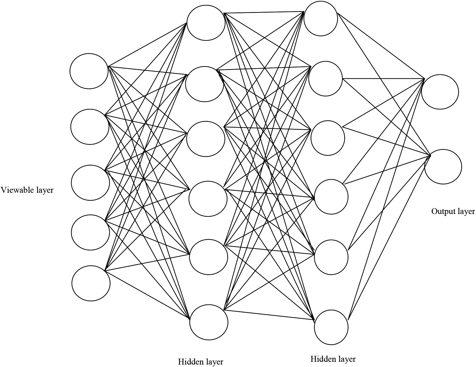

4. Results

The proposed work was implemented in Python and the dataset used in this work is the Malignant vs. Benign (ISIC) dataset.

Dataset Description: Images of both benign as well as malignant skin moles are evenly distributed across this dataset. Two files containing 1800 images (224x244) of each of the two varieties of moles make up the data.

Dataset description

Our Arithmetic Operated Honey Badger Algorithm (AOHBA) based skin cancer detection performance matrices were compared with diverse conventional systems such as WOA, SSA, HBA, TOA, and AOA, and the findings were given below.

Image results obtained from the original image, pre-processing, segmentation phases, FCM image, and K-means are given in Figs 5–10 with sample images.

Figure 5.

Image results obtained from Sample images.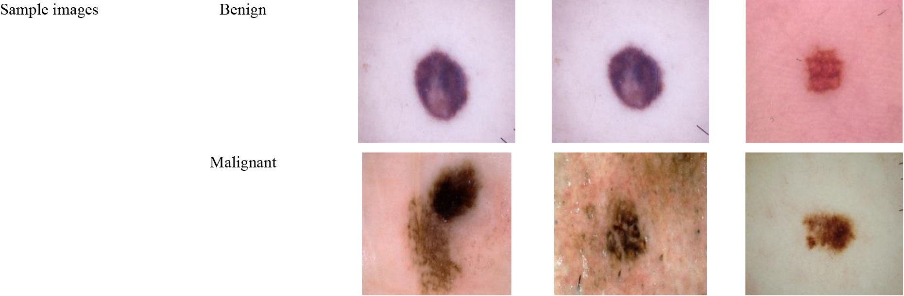

Figure 6.

Image results obtained from Pre-processed images.

Figure 7.

Image results obtained from Segmented images.

Figure 8.

Image results obtained from FCM images.

Figure 9.

Image results obtained from K-means images.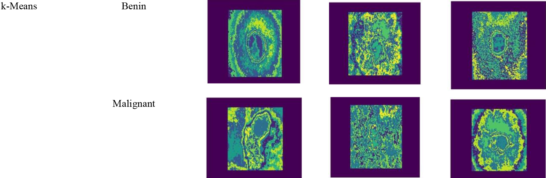

Figure 10.

Image results obtained from conventional BRICH images.

4.1 Dice score and Jacquard coefficient analysis

To prove the effectiveness of the skin cancer detection strategy, we have evaluated the matrices such as Dice-score and Jacquard coefficient analysis like the proposed BRICH, K-Means, and FCM. The proposed BRICH has attained the values of 0.681, 0.655, and 0.609 in the Dice score values. Jacquard coefficient analysis has achieved 0.80, 0.84, and 0.72 respectively. The comparison of segmentation methods is illustrated in Table 1.

Table 1
Conventional segmentation methods with Dice score and Jacquard coefficient analysis

Metrics	Measures	Prop-Brich	K-means	FCM
Dice score	Image 1	0.681304	0.601128	0.569618
	Image 2	0.65516	0.60085	0.582021
	Image 3	0.60953	0.57833	0.611647
Jacquard coefficient	Image 1	0.802968	0.759226	0.80853
	Image 2	0.842693	0.685941	0.840999
	Image 3	0.727307	0.67073	0.716907

Our proposed AOHBA’s cost function was assessed for 0–50 iterations, and the outcomes were contrasted with those of the existing algorithms shown in Fig. 11. The cost function values for WOA and SSA are 1.153 and 1.165 for 0–10 iterations, respectively, but the value for our AOHBA technique is 1.133. Our proposed AOHBA method’s cost function value is low and steady after 10 iterations and is equal to 1.1. From the graph, the proposed AOHBA has attains the minimization error ranges from 1.15 to 1.09 demonstrating its effectiveness.

Figure 11.

Cost function comparison of proposed AOHBA with conventional algorithms for 0–50 iterations.

Figure 12 compares the outcomes of our proposed AOHBA’s evaluation of performance metrics including accuracy, precision, sensitivity, as well as specificity with those of traditional algorithms for learning percentages of 60 to 90. In comparison to other traditional approaches, our proposed AOHBA achieves rates of 0.88, 0.9, 0.9, and 0.8 at 60 LP, whereas WOA and TOA only achieve accuracy, precision, sensitivity, and specificity values of 0.78, 0.85, 0.72, and 0.79, and 0.88, 0.82, and 0.79, respectively. The fact that our proposed AOHBA technique simultaneously obtains higher measure values for 70, 80, as well as 90 LPs demonstrates the higher performance of our proposed AOHBA approach.

In a similar manner, the outcomes of our proposed AOHBA technique for 60–90 LPs were analyzed for performance metrics such as F measure, MCC, NPV, FNR, as well as FPR, and the comparisons with standard methods are shown in Fig. 13. While our proposed AOHBA meets the rate of 0.9, 0.83 and 0.93 at 70 LP, SSA, and HBA attain the f measure, MCC, as well as NPV measure values of (0.82, 0.61 and 0.7) and (0.82, 0.62 and 0.71), respectively. The reality that our proposed AOHBA-based skin cancer detection methodology receives higher ratings for 80 and 90 LPs, respectively (0.96, 0.96, and 0.97) and (0.97, 0.97, and 0.97), shows that it can function more adequately than other classical methodologies. Our proposed AOHBA also attains a rate of (0.100, 0.050, 0.040, and 0.050) as well as (0.20, 0.15, 0.10, 0.10) for negative matrices like FNR and FPR assessment, that’s less than other standard methodologies.

Table 2

Performance comparison of ablation study with four scenarios

Matrices	Conventional BIRCH	Conventional LVP	Without feature selection	Conventional DBN	AOHBA
Accuracy	0.810025	0.887917	0.808676	0.835907	0.917932
Sensitivity	0.832622	0.902366	0.8314	0.855972	0.940636
Specificity	0.768322	0.860365	0.766762	0.798471	0.875659
Precision	0.868984	0.924942	0.867986	0.887945	0.933708
F_measure	0.850415	0.913515	0.849299	0.871665	0.937159
MCC	0.591511	0.754846	0.588725	0.645234	0.81896
NPV	0.713241	0.822101	0.71145	0.74821	0.887926
FPR	0.231678	0.139635	0.233238	0.201529	0.124341
FNR	0.167378	0.097634	0.1686	0.144028	0.059364

Figure 12.

Comparison of performance matrices including Positive measures.

Figure 13.

Comparison of performance matrices for negative and neutral measures.

In this work, an ablation study was carried out to examine the effectiveness of our proposed AOHBA-based skin cancer detection system by eliminating specific processes in order to determine their relative contributions to the system as a whole. Our proposed AOHBA is employed in four scenarios: conventional BIRCH, conventional LVP, conventional DBN, as well as convenient operation without feature extraction. Table 2 lists the performance metrics for each scenario.

In order to determine the efficacy of our improved BIRCH and improved LVP, the proposed method was tested against conventional BIRCH and LVP, which obtained accuracy rates of 0.8100 and 0.8879, respectively, while our proposed obtained a rate of 0.9179, demonstrating that we can obtain better results by using our improved BIRCH and LVP. Similarly, our proposed AOHBA achieves the sensitivity and specificity rates of 0.9406 and 0.8756, whereas the approach without feature extraction only manages to attain rates of 0.8314 and 0.7667. The MCC and NPV values achieved while employing conventional DBN were 0.6452 and 0.7482, however, our proposed AOHBA obtains rates of 0.8189 and 0.8879, which are greater than other scenarios.

The outcomes of the comparisons between our proposed AOBHA’s various performance metrics with several classifiers, including SVM, RF, KNN, CNN, as well as DBN, are seen in Table 3. In contrast to the accuracy rates of 0.7736, 0.8050, and 0.7899 achieved by SVM, KNN, and RF classifiers, our proposed AOBHA-based skin cancer detection method obtains a rate of 0.9179. Our proposed AOBHA also yields rates of 0.9406 & 0.8756 in terms of sensitivity and specificity, whereas CNN and DBN classifiers reach rates of 0.9142, 0.8256 and 0.8559, 0.7984, which are lower than our proposed AOBHA-based skin cancer detection approach.

Table 3

Performance comparison of our proposed AOBHA with conventional classifiers

	SVM	RF	KNN	CNN	DBN	AOHBA
Accuracy	0.773691	0.789907	0.805004	0.882677	0.835907	0.917932
Sensitivity	0.828861	0.841931	0.928942	0.914224	0.855972	0.940636
Specificity	0.682796	0.703024	0.635444	0.825693	0.798471	0.875659
Precision	0.811502	0.825618	0.777091	0.904526	0.887945	0.933708
F_measure	0.82009	0.833695	0.846258	0.909349	0.871665	0.937159
MCC	0.515435	0.54878	0.603069	0.743214	0.645234	0.81896
NPV	0.70774	0.727013	0.867312	0.842	0.74821	0.887926
FPR	0.317204	0.296976	0.364556	0.174307	0.201529	0.124341
FNR	0.171139	0.158069	0.071058	0.085776	0.144028	0.059364

Statistical measures of our proposed AOHBA were evaluated in terms of error and are compared with various optimization algorithms such as WOA, TOA, SSA, AOA, and HBA, which are given in Table 4. The STD as well as mean values of the WOA, and TOA were 0.019, 1.133, and 0.0179, 1.117, respectively, which were higher than our proposed AOHBA of 0.014, and 1.113. When AOA and HBA achieve maximum and minimum values of 1.1569, 1.1059, and 1.1507, 1.1072, respectively, our proposed AOHBA achieves rates of 1.1501 and 1.1049, indicating that our proposed AOHBA can give fewer error outputs than the other classical approaches. This evaluation is done as the model relies on the use of an optimization algorithm. Normally, optimization algorithms are stochastic in nature, and thereby evaluation is needed to determine the optimal performance with respect to statistical measures. In this work, the evaluation is carried out with respect to certain case scenarios.

Table 4

Statistical analysis of proposed and convention

Method	Statistical measures
	Standard deviation (STD)	Mean	Median	Max	Min
WOA	0.019109	1.13304	1.122223	1.182589	1.115315
TOA	0.017929	1.117486	1.106982	1.148479	1.106982
SSA	0.020896	1.122828	1.109454	1.167911	1.109454
AOA	0.016095	1.114988	1.105933	1.156963	1.105933
HBA	0.018022	1.120034	1.107233	1.150772	1.107233
AOHBA	0.014266	1.111375	1.104983	1.150126	1.104983

5. Conclusion

The input photos are pre-processed in the initial pre-processing stage using Gaussian filtering as well as histogram equalization methods. Improved Balanced Iterative Reducing and Clustering Using Hierarchies (I-BIRCH) was created to improve image segmentation by effectively assigning labels to pixels. In the third step, features including Improved Local Vector Pattern, local ternary pattern, Grey level co-occurrence matrix, and local gradient patterns were retrieved from the segmented images. We created an Arithmetic Operated Honey Badger Algorithm (AOHBA) for feature selection, which lowered computational costs and training time by picking the optimal features from the retrieved features. Finally, the photos are categorized utilizing an improved Deep Belief Network (DBN) based on the selected features, and the performance assessment results are compared to traditional techniques to demonstrate the efficacy of our proposed skin cancer detection strategy.

Footnotes

Author’s Bios

	Jinu P. Sainudeen was born in Kerala, India. She received the Bachelor’s degree in Information Technology from Cochin University of Science and Technology, Kerala in 2006, and the M.Tech degree in Computer and Information Technology from M.S University, Thirunelveli, in 2012. She is currently pursuing the PhD degree in Hindustan Institute of Technology and Science, Chennai. Her key research interests include medical, clinical, and biological-image data analysis, with the application of image processing, computer vision, machine learning and deep learning. Her profound interest in research has made her to publish various papers and articles. She has also participated in various workshops and conferences. She has been with Mangalam College of Engineering since 2006. Now working as associate professor in the department of Computer Science and Technology. She is a dedicated and student-focused teaching professional and is committed in providing a well-balanced, supportive and learning environment to students.
	Ceronmani Sharmila V, Professor & Head – Department of Information Technology in Hindustan Institute of Technology and Science, Chennai. She has received her PhD from Hindustan Institute of Technology andScience, Chennai. She has received her B.E in Electronics and Communication from Madras University, Chennai and M.E in Communication Systems from Anna University, Chennai. She is a motivating and talented Professor, driven to inspire students to pursue academic, research, and personal excellence, consistently strive to create a challenging and engaging learning environment in which students become lifelong scholars and learners. She has exceptional track record of research success with multiple published articles in peer-reviewed journals. Her key research interests include Cyber Security, Computer Networks (Mobile Ad Hoc and Sensor Networks), Image Processing, Cloud Security, Deep Learning, Internet of Things (IoT), Applications of Graph Theory and Very Large Scale Integration (VLSI).
	Parvathi R, Associate Professor – Department of Information Technology in Hindustan Institute of Technology and Science, Chennai. She has received her PhD from Anna University, in 2016. She has received her B.E in Information Technology from Anna University, in 2005 and M.E in Computer Science and Engineering from Anna University, in 2010. She has 16 years of academic experience.Her research interestsinclude Biometrics, Machine Learning, Cyber Security, Internet of Things. She got funded project from AICTE under RPS scheme. She has published 40 journals. She has acted as various committee member.

References

Mirbeik-Sabzevari

Ashinoff

and Tavassolian

, Ultra-wideband millimeter-wave dielectric characteristics of freshly excised normal and malignant human skin tissues, IEEE Transactions on Biomedical Engineering 65 (2017), 1320–1329.

Gálvez

J.M.

Castillo-Secilla

Herrera

L.J.

Valenzuela

Caba

Prados

J.C.

and Rojas

, Towards improving skin cancer diagnosis by integrating microarray and RNA-seq datasets, IEEE Journal of Biomedical and Health Informatics 24 (2019), 2119–2130.

Adegun

A.A.

and Viriri

, FCN-based DenseNet framework for automated detection and classification of skin lesions in dermoscopy images, IEEE Access 8 (2020), 150377–150396.

Navarro

Escudero-Vinolo

and Bescós

, Accurate segmentation and registration of skin lesion images to evaluate lesion change, IEEE Journal of Biomedical and Health Informatics 23 (2018), 501–508.

Arab

Chioukh

Ardakani

M.D.

Dufour

and Tatu

S.O.

, Early-stage detection of melanoma skin cancer using contactless millimeter-wave sensors, IEEE Sensors Journal 20 (2020), 7310–7317.

Ashraf

Afzal

Rehman

A.U.

Gul

Baber

Bakhtyar

and Maqsood

, Region-of-interest based transfer learning assisted framework for skin cancer detection, IEEE Access 8 (2020), 147858–147871.

Goyal

Oakley

Bansal

Dancey

and Yap

M.H.

, Skin lesion segmentation in dermoscopic images with ensemble deep learning methods, IEEE Access 8 (2019), 4171–4181.

Khan

M.Q.

Hussain

Rehman

S.U.

Khan

Maqsood

Mehmood

and Khan

M.A.

, Classification of melanoma and nevus in digital images for diagnosis of skin cancer, IEEE Access 7 (2019), 90132–90144.

Pham

T.C.

Doucet

Luong

C.M.

Tran

C.T.

and Hoang

V.D.

, Improving skin-disease classification based on customized loss function combined with balanced mini-batch logic and real-time image augmentation, IEEE Access 8 (2020). 150725–150737.

10.

Xie

Zhang

Xia

and Shen

, A mutual bootstrapping model for automated skin lesion segmentation and classification, IEEE Transactions on Medical Imaging 39 (2020), 2482–2493.

11.

Kawahara

Daneshvar

Argenziano

and Hamarneh

, Seven-point checklist and skin lesion classification using multitask multimodal neural nets, IEEE Journal of Biomedical and Health Informatics 23 (2018), 538–546.

12.

Mahmouei

S.S.

Aldeen

Stoecker

W.V.

and Garnavi

, Biologically inspired quadtree color detection in dermoscopy images of melanoma, IEEE Journal of Biomedical and Health Informatics 23 (2018), 570–577.

13.

Albahli

Nida

Irtaza

Yousaf

M.H.

and Mahmood

M.T.

, Melanoma lesion detection and segmentation using YOLOv4-DarkNet and active contour, IEEE Access 8 (2020), 198403–198414.

14.

Celebi

M.E.

Codella

and Halpern

, Dermoscopy image analysis: Overview and future directions, IEEE Journal of Biomedical and Health Informatics 23 (2019), 474–478.

15.

Ahmad

Usama

Huang

C.M.

Hwang

Hossain

M.S.

and Muhammad

, Discriminative feature learning for skin disease classification using deep convolutional neural network, IEEE Access 8 (2020), 39025–39033.

16.

Jiang

Cao

Tao

and Zhang

, Skin lesion segmentation based on multi-scale attention convolutional neural network, IEEE Access 8 (2020), 122811–122825.

17.

Hagerty

J.R.

Stanley

R.J.

Almubarak

H.A.

Lama

Kasmi

Guo

and Stoecker

W.V.

, Deep learning and handcrafted method fusion: Higher diagnostic accuracy for melanoma dermoscopy images, IEEE Journal of Biomedical and Health Informatics 23 (2019), 1385–1391.

18.

Naeem

Farooq

M.S.

Khelifi

and Abid

, Malignant melanoma classification using deep learning: Datasets, performance measurements, challenges and opportunities, IEEE Access 8 (2020), 110575–110597.

19.

Song

Lin

Wang

Z.J.

and Wang

, An end-to-end multi-task deep learning framework for skin lesion analysis, IEEE Journal of Biomedical and Health Informatics 24 (2020), 2912–2921.

20.

Kassem

M.A.

Hosny

K.M.

and Fouad

M.M.

, Skin lesions classification into eight classes for ISIC 2019 using deep convolutional neural network and transfer learning, IEEE Access 8 (2020), 114822–114832.

21.

Wang

Jiang

Ding

and Liu

, Bi-directional dermoscopic feature learning and multi-scale consistent decision fusion for skin lesion segmentation, IEEE Transactions on Image Processing 29 (2019), 3039–3051.

22.

Adegun

A.A.

and Viriri

, Deep learning-based system for automatic melanoma detection, IEEE Access 8 (2019), 7160–7172.

23.

Yuan

and Lo

Y.C.

, Improving dermoscopic image segmentation with enhanced convolutional-deconvolutional networks, IEEE Journal of Biomedical and Health Informatics 23 (2017), 519–526.

24.

Gong

Yao

and Lin

, Classification for dermoscopy images using convolutional neural networks based on the ensemble of individual advantage and group decision, IEEE Access 8 (2020), 155337–155351.

25.

Saba

Khan

M.A.

Rehman

and Marie-Sainte

S.L.

, Region extraction and classification of skin cancer: A heterogeneous framework of deep CNN features fusion and reduction, Journal of Medical Systems 43 (2019), 1–19.

26.

Balaji

Saravanan

Chandrasekar

Rajkumar

and Kamalraj

, Analysis of basic neural network types for automated skin cancer classification using Firefly optimization method, Journal of Ambient Intelligence and Humanized Computing 12 (2021), 7181–7194.

27.

Thanh

D.N.

Prasath

V.B.

Hieu

L.M.

and Hien

N.N.

, Melanoma skin cancer detection method based on adaptive principal curvature, colour normalisation and feature extraction with the ABCD rule, Journal of Digital Imaging 33 (2020), 574–585.

28.

Murugan

Nair

S.A.H.

and Kumar

K.P.

, Detection of skin cancer using SVM, random forest and kNN classifiers, Journal of Medical Systems 43 (2019), 1–9.

29.

Kumar

Alshehri

AlGhamdi

Sharma

and Deep

, A de-ann inspired skin cancer detection approach using fuzzy c-means clustering, Mobile Networks and Applications 25 (2020), 1319–1329.

30.

Sreelatha

Subramanyam

M.V.

and Prasad

M.N.

, Early detection of skin cancer using melanoma segmentation technique, Journal of Medical Systems 43 (2019), 1–7.

31.

Thurnhofer-Hemsi

and Domínguez

, A convolutional neural network framework for accurate skin cancer detection, Neural Processing Letters 53 (2021), 3073–3093.

32.

Chaturvedi

S.S.

Tembhurne

J.V.

and Diwan

, A multi-class skin Cancer classification using deep convolutional neural networks, Multimedia Tools and Applications 79 (2020), 28477–28498.

33.

www.geeksforgeeks.org/apply-a-gauss-filter-to-an-image-with-python.

34.

https://www.geeksforgeeks.org/adaptive-histogram-equalization-in-image-processing-using-matlab.

35.

https://en.wikipedia.org/wiki/BIRCH.

36.

Hung

T.Y.

and Fan

K.C.

, Local vector pattern in high-order derivative space for face recognition, in: 2014 IEEE International Conference on Image Processing (ICIP), 2014.

37.

Reddy

K.S.

Kumar

V.V.

and Reddy

B.E.

, Face recognition based on texture features using local ternary patterns, International Journal of Image, Graphics and Signal Processing 7 (2015), 37.

38.

Shirke

S.D.

and Rajabhushnam

, Local gradient pattern and deep learning-based approach for the iris recognition at-a-distance, International Journal of Knowledge-based and Intelligent Engineering Systems 25 (2021), 49–64.

39.

Alazawi

S.A.

Shati

N.M.

and Abbas

A.H.

, Texture features extraction based on GLCM for face retrieval system, Periodicals of Engineering and Natural Sciences (PEN) 7 (2019), 1459–1467.

40.

Hashim

F.A.

Houssein

E.H.

Hussain

Mabrouk

M.S.

and Al-Atabany

, Honey Badger Algorithm: New metaheuristic algorithm for solving optimization problems, Mathematics and Computers in Simulation 192 (2022), 84–110.

41.

Abualigah

Diabat

Mirjalili

Abd Elaziz

and Gandomi

A.H.

, The arithmetic optimization algorithm, Computer Methods in Applied Mechanics and Engineering 376 (2021), 113609.

42.

Zhang

and Yu

, Remote sensing image land classification based on deep learning, Scientific Programming 2021 (2021).

43.

https://peltarion.com/knowledge-center/documentation/modeling-view/build-an-ai-model/loss-functions/mean-squared-error.

Skin cancer detection: Improved deep belief network with optimal feature selection

Abstract

Keywords

1. Introduction

3. Methodology

3.1.1 Gaussian filtering

3.2 Segmentation

3.3.1 Improved local vector pattern

3.4 Optimal feature selection

3.4.1 Arithmetic Operated Honey Badger Algorithm (AOBHA)

Dataset description

Table 1 Conventional segmentation methods with Dice score and Jacquard coefficient analysis

Footnotes

Author’s Bios

References

Table 1
Conventional segmentation methods with Dice score and Jacquard coefficient analysis