
Abstract
Accurate and early detection of plant disease is significant for stable and proper agriculture and also for preventing the unwanted waste of financial and other possessions. Hence, a new technique is devised in this work, where geese jellyfish search optimization trained deep learning is used for multiclass detection of plant disease utilizing plant leaf images. At first, the input leaves of the plant image acquired from the database are pre-processed utilizing the Kalman filter. Then, the plant leaf segmentation is done by LinK-Net, where the training function of LinK-Net is processed by the proposed geese jellyfish search optimization, which is formed using wild geese migration optimization and jellyfish search optimizer. Then, image augmentation is carried out and then the feature extraction is done. Consequently, the classification of plant leaf type is processed, which is employed by Deep Q-Network (DQN), which is structurally adapted by the proposed geese jellyfish search optimization. At last, multi-label plant leaf disease is detected based on DQN. Moreover, the proposed geese jellyfish search optimization based DQN obtains an accuracy of 89.44%, true positive rate of 90.18%, and false positive rate of 10.56% respectively.
Keywords
Introduction
Agriculture is only one of the main segments that contributes to the improvement of the Indian economy and is called the backbone of the Indian economy. At most 50% of Indian people’s occupation is based in the cultivation sector. To increase the outcome of agriculture, it is essential to identify the key information for plant disease so that the damage to harvest can be prevented [1]. The kinds of disease must be identified to avoid the spreading of the disease in the agricultural sector. In the early days, the disease is identified based on a visual examination of plant leaves’ symptoms, which creates a high degree of complexity in plant disease detection [2]. Misidentification of crop disease leads to the utilization of incorrect insecticides, which leads to a decrease in the nutrition efficiency in the agricultural sector [3]. The identification and solution of infections are necessary for enhancing the yield and growth of crops. An intellectual plant leaf disease identification technique is necessary to examine agricultural areas frequently [4]. Nowadays, some plant leaf disease identification techniques are devised for automatic plant disease identification utilizing Artificial Intelligence methods with low human participation [5, 6]. Based on the development of Artificial Intelligence, computer vision is required to integrate the facilities in the agriculture sector [7]. In agriculture management, the farmers are offered specialist knowledge depending upon a decision support system [8, 9]. The income and lifestyle of the farmers can be improved based on the quantity and superiority of the harvest. Both human and animal life depends on the plants [10].
The protection of plants from diseases plays an important part in satisfying the rising requirement for quality and quantity of food [11]. According to the Indian Council of Agricultural Research, more than 35% of crop production is affected by disease and pests [12]. Well-timed and correct identification of plant diseases is very important for sustainable and accurate agriculture [13]. The analysis of the disease of the plant leaf is not suitable for the revisions of the visibly perceptible outer layer supposed on the plant. Disease recognition and health observation on plants are truly serious for manageable cultivation [1]. The disease of the plant leaf is detected based on the image is a freshly investigated area by more researchers. Crop disease detection assists the farmers to learn about the cause of plant infections and get the prevention methods to treat the disease. Initial detection of plant disease depends on the color of the leaf, the size of the leaf, the growth of the pattern, and so on it helps farmers [7]. Some diseases require advanced examination techniques when the symptoms are not visible. However, a major amount of plant diseases portray visible symptoms and an experienced plant pathologist detects the disease via optical surveillance of disease-affected plant leaves [13]. However, the physical observation of plant disease is very difficult and it requires an unbelievable amount of endeavour plant disease detection requires too much computing period, so image-based treatment is used for the detection of plant disease [1].
Many conventional Machine Learning methods are devised for the classification and detection of plant diseases [13]. A large amount of research has been devised for crop disease identification and classification. The capability of machine learning techniques to solve real-time challenging issues is an incredible part of the intelligence of the human brain. The main problems of machine learning-based methods over the detection of crop disease are low efficiency and huge computation time as these frameworks create long lengthy codes, which increases the complexity of computation. In addition, the difference in brightness during the capturing of plant leaves image also complicates the identification method [14]. The utilization of deep learning methods in the detection and categorization of disease from images in medical is quite common. On another hand, deep learning-based studies for the classification and detection of plant diseases are utilized in numerous studies. But, still, it has some gaps in the examination regarding the utilization of particularly novel deep learning structures in the disease of plant leaves. Particularly, the necessity for effective methods with minimal parameters that can be trained quickly and without compromise on presentation is unavoidable [13]. Hyperparameters are the most important training parameters that can impact the process of deep learning methods. Random search and grid search are the most common hyperparameter tuning techniques in deep learning. High presentation processing power is required to train the deep learning algorithms with better efficiency and low execution time [15, 6].
The effective plant leaf disease classification is a primary contribution of this research paper and it is processed as follows. At first, the plant leaf image is taken from a plant village sampleset and it is preprocessed by the Kalman filter. Afterwards, the preprocessed image is subjected to the segmentation phase, where segmentation is employed by Link-Net, The weights and bias of the Link-Net are trained by the proposed geese jellyfish search optimization, which is the incorporation of geese migration optimization and jellyfish search optimizer. Consequently, image augmentation is performed and the augmentation applied image is allowed to feature extraction performance. Afterwards, plant-type classification is done by Deep Q-Network (DQN), which is trained by the proposed geese jellyfish search optimization. Finally, multiclass plant leaf disease is identified based on DQN, and it is trained by the proposed geese jellyfish search optimization.
The main key contribution of this paper is explained below, proposed geese jellyfish search optimization based DQN for disease detection of plant leaf: Here, the devised geese jellyfish search optimization based DQN is applied for multiclass plant disease detection, where geese jellyfish search optimization is the incorporation of geese migration optimization and jellyfish search optimizer. In this paper, Link-Net trained by geese jellyfish search optimization is employed for segmentation. Then, DQN trained by geese jellyfish search optimization is utilized for plant leaf type classification and detection.
The rest portion of this study is organized as below: Part 2 depicts a literature review of traditional techniques with their limitations and advantages. Part 3 indicates the proposed geese jellyfish search optimization based DQN and its performance, Part 4 signifies the proposed scheme’s outcome and experimental study and the work is concluded in Part 5.
Literature review
Atila et al. [13] devised an EfficientNet deep learning structure for the identification of disease-affected plants. This technique achieved more effective outcomes by uniformly detecting width, resolution, and scaling depth, although this technique had maximum execution time. Ahmed and Reddy [3] developed a Convolution Neural Network (CNN) for the detection of crop disease symptoms and this algorithm performed superior results with less computation complexity, but this technique did not perform well on leaf images with complex backgrounds. Albattah et al. [14] introduced the DenseNet-77 for the detection of plant disease. Here, the identification of disease was more effective and the method identified the disease location of the plant leaf but this technique was easily affected by the overfitting problem. Vallabhajosyula et al. [16] devised the Deep Ensemble Neural Networks (DENN) for the identification of plant disease. This algorithm decreased training function and convergence time and tuned the huge amount of parameters effectively, although this technique failed to process some parameters, such as epochs, learning rate, activation functions, etc. to enhance efficiency. Pandian et al. [6] devised the Deep CNN for the detection of plant disease. Here, the overall efficiency of the technique was improved, because of the use of rotation, flipping, and cropping. However, this technique failed to identify the disease in the other portions of a plant like fruits, stems, and flowers. Chouhan et al. [10] developed the Internet of Things – Fuzzy Based Function Network for the detection of plant disease. Here, the computational cost and computational power of the architecture were minimal, but it failed to incorporate technologies like big data, the Internet of Things, GPS, Unmanned Aerial Vehicle, devices like sensors cameras, etc. Mahum et al. [17] developed an Efficient DenseNet for detection of plant leaf disease and this technique was flexible enough and can be simply fine-tuned. But this technique was unfeasible, because of high execution time. Pandian et al. [18] introduced the Deep CNN for plant disease detection and this technique was also performed in the real-time dataset, but this technique had a high computational cost.
Proposed geese jellyfish search optimization based Deep Q-Network for plant disease detection
The plant leaf type and disease classification is a major goal of this study, where the proposed geese jellyfish search optimization based Deep Q-Network (DQN) was introduced for the classification of plant leaves. The input leaf image is taken from the dataset and it is allowed to a preprocessing phase. In preprocessing, the Kalman filter is used to remove an error from the input. Then, the plant leaf segmentation is processed by Link-Net [19] which is trained by the proposed geese jellyfish search optimization and it is designed by the integration of geese migration optimization [20] and jellyfish search optimizer [21]. Afterwards, the segmented output is allowed for image augmentation, where the data sample is increased based on translation, resize, contrast, resize, hue, and saturation. Then, feature extraction is performed, wherein features are Complete Local Binary Pattern (CLBP) features [22] and statistical features [23] are processed. Here, classification is based on first-level and second level classification. At first, plant leaf type is classified using DQN [24], and DQN is trained by the proposed geese jellyfish search optimization developed by the combination of geese migration optimization [20] and jellyfish search optimizer [21]. Finally, plant leaf disease is identified, which is done by DQN, which is trained by the proposed geese jellyfish search optimization under the integration of geese migration optimization [20] and jellyfish search optimizer [21]. Figure 1 signifies the structural diagram of the proposed geese jellyfish search optimization based DQN.
Structural diagram of the proposed geese jellyfish search optimization based deep Q-network for plant disease detection.
Consider the plant leaf image as input and it is accumulated from a dataset
where
The input plant leaf image
Kalman filter
For using the Kalman filtering [25] technique, disregard the organized inputs and process noise, the state and its interrelated covariance matrix for the following iteration, which is achieved optimum solution. The advantage of the Kalman filter is preserved low power and it is computationally effective. The Kalman filter is designed by,
where
The pre-processed plant image
Structure of Link-Net
The structure of Link-Net [19] is portrayed in Fig. 2, where the input of Link-Net is
Structure of Link-Net.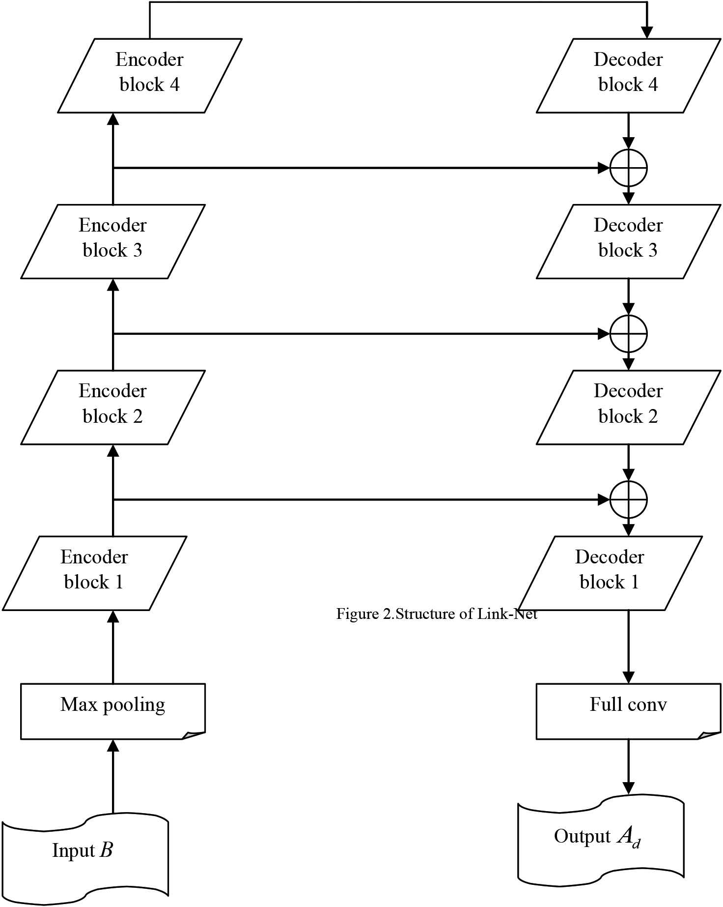
The plant leaf segmentation is carried out by Link-Net, which is structurally adapted by geese jellyfish search optimization, which is designed by integration of geese migration optimization [20] and jellyfish search optimizer [21]. To improve the segmentation accuracy both the algorithm is combined and used to train the Link-Net. The geese migration optimization [20] is simple and a minimum number of parameters are used. It performed excellently in terms of computation cost and computational power. The jellyfish search optimizer [21] is utilized to solve the structural optimization issue efficiently. An efficient tradeoff between intensification and diversification assists in decreasing the cost of computation and employs effective optimization. The below steps explain the realization of the geese jellyfish search optimization.
1) Population initialization
Normally, the population is initialized randomly in any optimization algorithm, and it endures local optima. The population initiation is formulated as,
where the position of
2) Evaluation of fitness solution
The fitness solution is estimated based on the Mean Square Error (MSE), which is designed as,
where the whole amount of training sample is denoted as
3) Ocean current
Huge amounts of nutrients are contained in ocean current, so jellyfish are intent by it, where the current best position is determined based on the ocean current direction by all vectors averaging and it is formulated by,
where the current best position of the jellyfish swarm is represented as
where
To improve convergence speed geese migration optimization [21] is added to jellyfish search optimizer, and from the geese migration optimization,
Substituting Eq. (10) in Eq. (6),
where
4) Swarm of jellyfish
Jellyfish swarm undertakes active (Type A) and passive (Type B) motions, where mostly jellyfish signify type A motion, and the consequent upgraded position of every jellyfish is expressed as,
where
Considering the Type B motion, where the displacement of efficient exploitation of a local search space is expressed as,
Hence the updated position is given by,
where the objective function of the position
5) Mechanism of time control
This situation introduced the mechanism of time control, which normalizes the movement between the jellyfish and ocean current depend on inside a swarm of jellyfish, the time control function
where Maxiter represents the iteration of the maximum number, which is parameter initialization.
6) Boundary condition
Around the world, the ocean is located and the earth is roughly spherical, so jellyfish move outside the bounded search area and return to the opposite bound, and this is modelled as.
7) Feasibility estimation
The position of every population is updated due to the roles of a proposed technique and the new position is evaluated.
8) Termination
The phases are repetitively executed till the highest iteration is achieved.
Image augmentation is a function of creating novel transformed versions of images from the acquired image dataset to raise its diversity, wherein augmentation techniques like resizing, shearing, translation, contrast, saturation, and hue are performed [26, 27]. Here, the outcome of segmentation
1) Resizing
Resize [26] is an image augmentation technique, which is used to adjust the longest length of the edge, which maintains the aspect ratio of the input image also the shortest edge is modified as per the required size, and the resized output is denoted as
2) Shearing
Shearing [27] is a process of modifying the image direction along the x and y directions, which contains the two phases. The component in the x-axis is the first phase and the component in the y-axis is the second phase and the following expressions are explained in the x and y direction shearing.
where after shearing new location of every pixel is denoted as
3) Translation
The movement of an object from horizontal and vertical directions in the image is called translation, where a geometric image is translated based on black or white. The translation can be performed based on X and Y directions at the same time [27]. To avoid the locational weights in data, the picture can be translated in left, down, right, and up directions and the equation of translation is expressed as,
where after translation, the new location of every pixel is denoted as
4) Contrast
The separation of dark and white color from an image is indicted contrast, which is used to control the amount of jitter based on the value 0 (no modification) and value 1 (gradually large modification). It specified only the prospective strength of the effect but did not include the higher and lower levels of the image [26]. The contrast adjusted image is denoted as
5) Saturation
The random saturated jitter is added to the image to improve the color quality of the image, which is based on the amount of color in an image [26]. The parameter is utilized to manage the quantity of jitter in saturation based on the value 0 (no modification) and value 1 (gradually large modification), where saturation is specified only the prospective strength of the effect but does not include the higher and lower level of the image, and the outcome is denoted as
6) Hue
Add random hue jitter from the image is hue applied image, which is based on the color shade of the image [26]. To control the quantity of jitter, the parameter hue is used with the value 0 and value 1, and the hue augmented image is indicated as
The images generated by applying various approaches are combined and the overall image produced by the augmentation is expressed as,
The image augmentation output
Complete Local Binary Pattern (CLBP)
To code the local image in a more absolute manner [22], the CLBP is devised for texture classification. The dissimilarity between the neighborhood pixels is denoted as
where
where
Statistical features
Here, CLBP output
1) Mean
The mean represents the concentration of the data distribution [23] and is expressed as
where
2) Variance
The variance of the grey-level image is related to the deviation of the grey-level image from the mean and the variance [23] of the grey-level image is formulated by,
where
3) Standard deviation
The standard deviation [23] represents the distribution of data about the mean value, whereas a low standard deviation depicts the values that are many closeups to the mean, and a high standard deviation represents a large dispersion of values among the mean. The standard deviation is formulated as,
where
4) Entropy
Entropy [23] is a measurement of information between the segmented image and classified image and it is formulated as,
where
5) Skewness
The asymmetrical distribution [23] of a particular feature about the mean is called skewness, which has negative or positive values and is computed as
where
6) Energy
The energy [23] is based on the second-order statistical features, which are formulated by Gray-Level Co-Occurrence Matrix (GLCM) squared components and it is expressed as
where
7) Contrast
Here, the intensity difference between each pixel and its neighborhood pixel is calculated [23] and is termed contrast and it is expressed as,
where contrast is represented as,
8) Correlation
The pixel value of the image is connected with its neighbourhood [23], which is called correlation and it is expressed as
where
Then, the features are concatenated to form the feature vector and the expression is
where
The type of plant leaf is classified by DQN, where feature extraction output
Architecture of Deep Q-Network (DQN)
The most commonly used reinforcement learning algorithm is called Q-learning, and itis used as the DQN [24] function also Q-function’s active value function is approximately calculated by CNN. Sometimes Reinforcement learning is represented as an unstable or nonlinear function that approximates divergence and an active value function is used for Neural Network representation. Moreover, DQN consists of convolution, dropout, max-pooling, flattening, and dense layers.
The convolution layer is a simple application of an input filter and has an activation. Here, the frequent application of an identical filter to an input outcome in an activation map is denoted as a feature map, demonstrating the positions and potency of an identified feature in an input, such as an image. Then, the function of the pooling layer is to reduce the dimension of the hidden layer by combining the outputs of neuron clusters at the before layer into a single neuron in the consequent layer. A flattened layer can be utilized to exchange semi-structured information for a representation of relationships. A dense layer is utilized to categorize images based on the outcome from convolution layers. Figure 3 portrays the structure of DQN.
Structure of Deep Q-Network (DQN).
The type of plant leaf is classified using DQN, trained by geese jellyfish search optimization, and it is designed combination of geese migration optimization [20] and jellyfish search optimizer [21]. A structural adaptation process is expanded in section 3.3.2 and
where the accepted outcome is indicated as
After classifying the plant leaf, the output
The plant disease detection is carried out by DQN, where leaf-type classified output
Architecture of Deep Q-Network (DQN)
DQN [24] is utilized for the identification of plant leaf disease and it is detailed in section 3.6.1. Here, plant leaf type classification outcome
Training function of Deep Q-Network (DQN) by geese jellyfish search
The plant disease detection is carried out by DQN, where plant disease classification outcome
where
The results of the proposed geese jellyfish search optimization based DQN for plant leaf disease classification and detection are illustrated in this portion. The evaluation of performance metrics, examination and dataset description, experimental arrangement, and comparative techniques are detailed in this part. Table 1 show the nomenclature used in the proposed work.
Nomenclature
Nomenclature
The proposed geese jellyfish search optimization based DQN for the detection of plant leaf disease is implemented with the Python tool employing the Plant Village dataset [28]. The multilevel classification of plant leaf disease is carried out using images from the Plant Village dataset [28]. In the plant village image, a different version of an image, such as the raw image’s greyscale version, RGB images with colour accustomed, and leaves segmented images are obtained. The total images in the dataset are 13294. Here, plant leaf images contained the total images of plants, like cherry with total image 1906, total apple images 3171, total tomato images of 4500, total image of potato is 2152, and total image of strawberry is 1565.
Evaluation measures
The efficacy of the proposed geese jellyfish search optimization based DQN is evaluated using metrics like accuracy, True Positive Rate (TPR), and False Positive Rate (FPR).
1) Accuracy
The effectiveness of plant disease detection and classification is examined utilizing accuracy, which is calculated based on the proportion between the correctly detected image to the whole quantity of taken image and it is formulated by,
where accuracy represents
2) True Positive Rate (TPR)
TPR determines the number of positive images, which are perfectly obtained out of a large quantity of positive image samples, and is given by,
where TPR is represented as
Experimental outcome of geese jellyfish search optimization based Deep Q-Network.
3) False Positive Rate (FPR)
FPR is formulated by the total amount of normal images classified as positive and the whole amount of normal images, which is expressed by,
where
Comparative examination of geese jellyfish search optimization based Deep Q-Network based on first-level classification.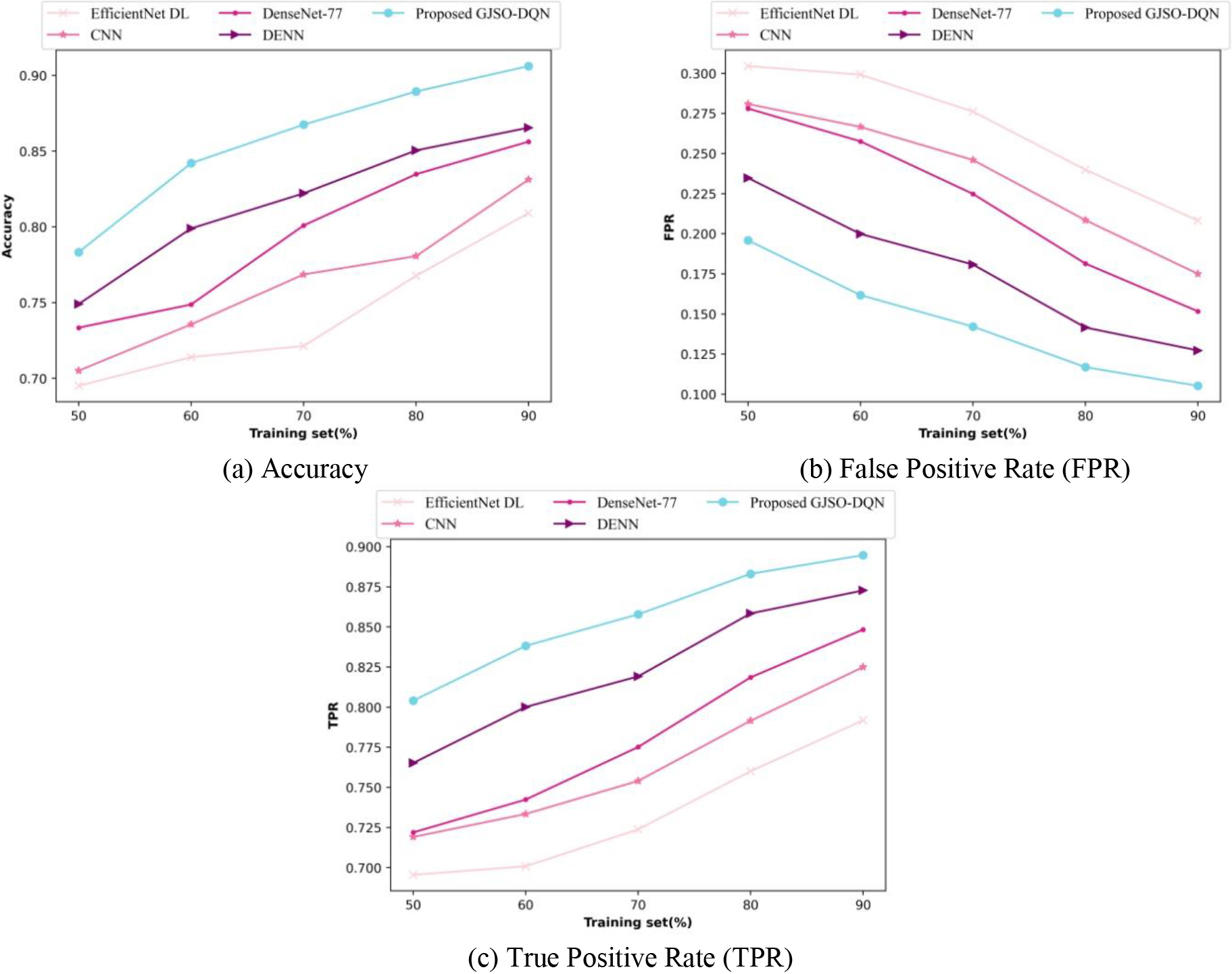
Comparative examination of geese jellyfish search optimization based Deep Q-Network based on first-level classification.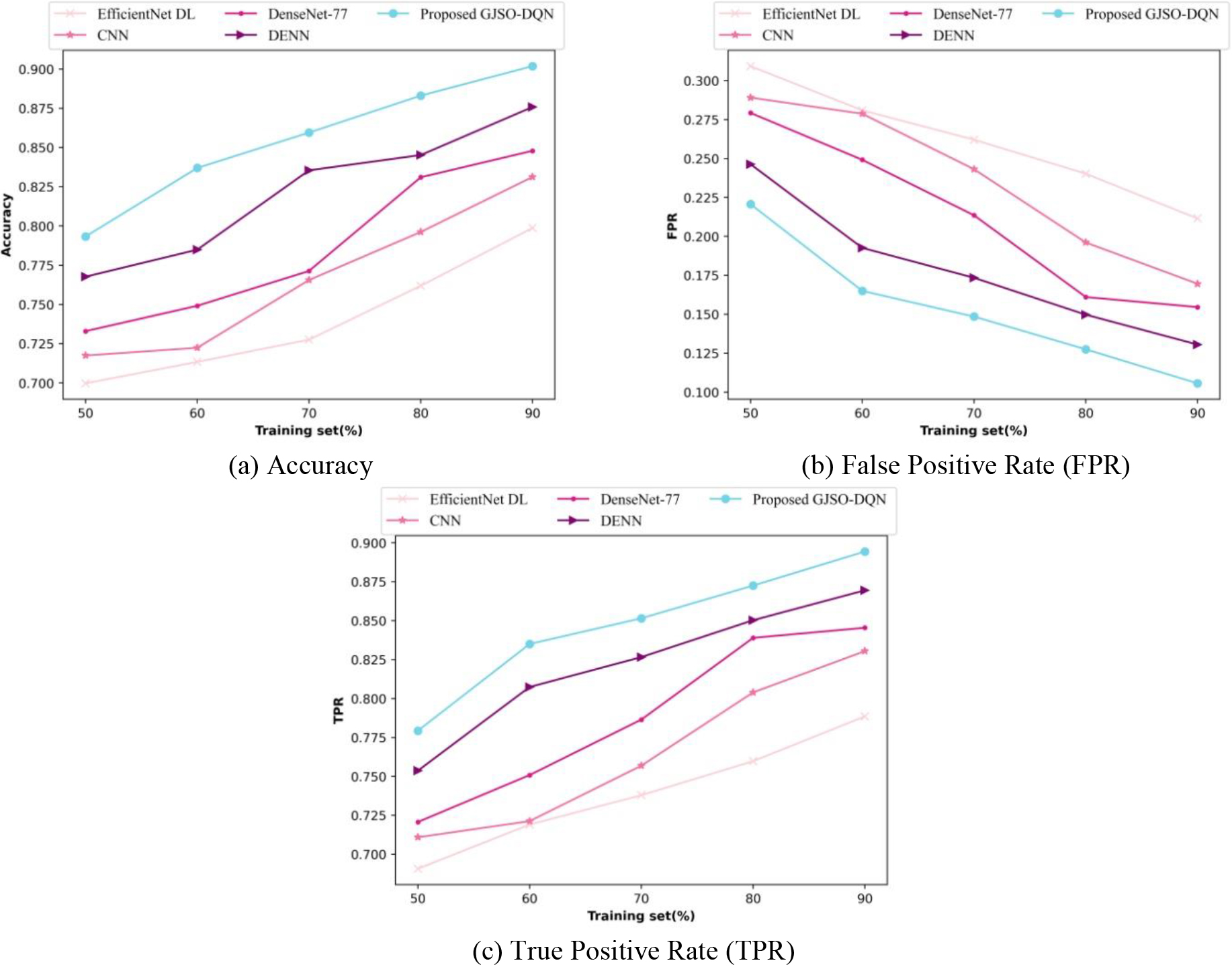
Performance examination of proposed geese jellyfish search optimization based Deep Q-Network based on first-level classification.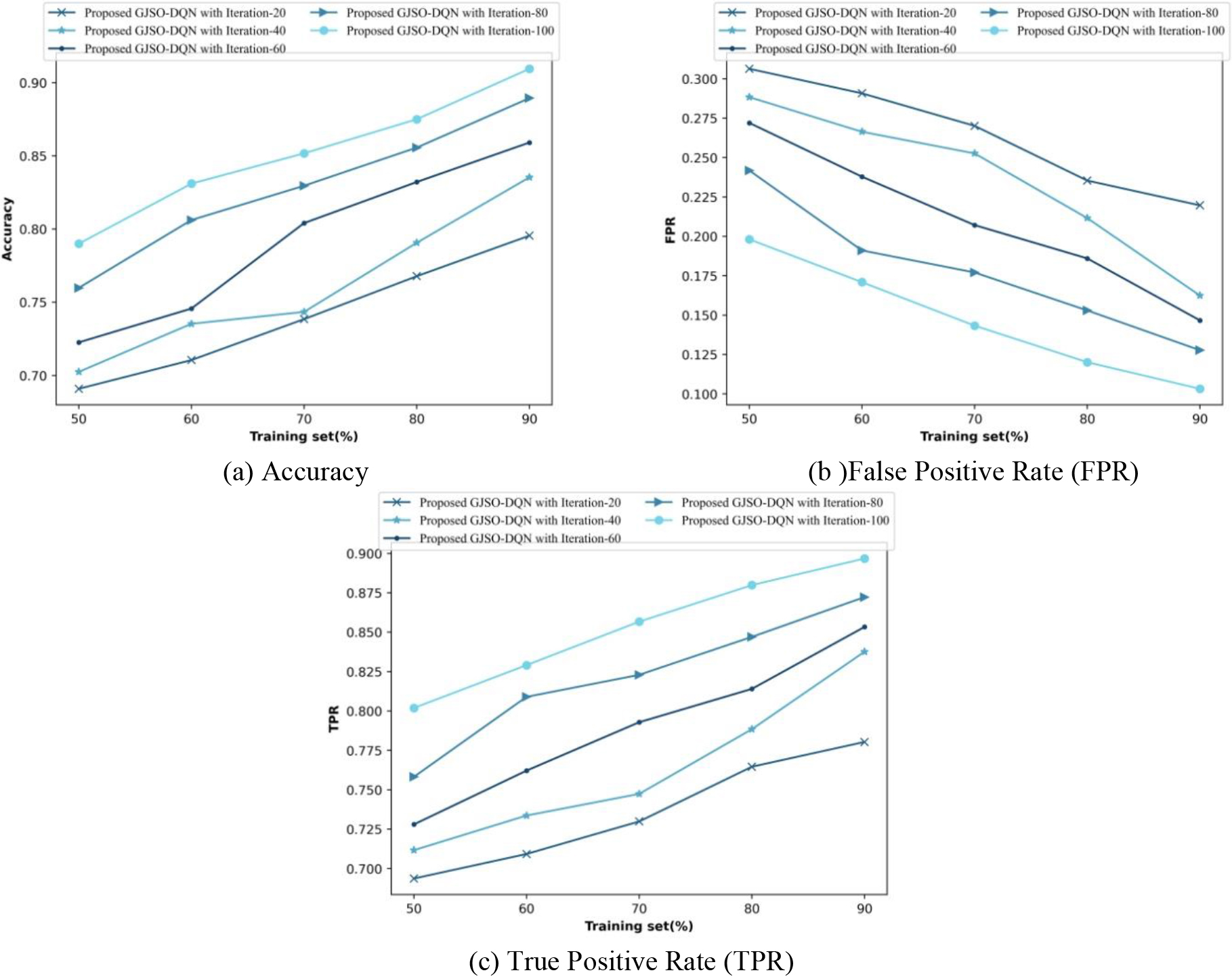
Performance examination of geese jellyfish search optimization based Deep Q-Network based on first-level classification.
Figure 4 indicates the experimental outcome of the proposed geese jellyfish search optimization based DQN for plant disease detection. Figure 4a indicates the input leaf image, Fig. 4b represents the pre-processed image, Fig. 4c shows the plant leaf segmented image, consequently, Fig. 4d–i, show the resized image, sheared image, translated image, contrast applied image, saturated image, and hue applied images, and also Fig. 4j–o indicates the CLBP based resized image, CLBP based sheared image, CLBP based translated image, CLBP based contrast applied image, CLBP based saturated image, and CLBP based hue processed images.
Comparative analysis
Various comparative methods, like EfficientNet Depp Learning (DL) [13], CNN [3], DenseNet-77 [14], and Deep Ensemble Neural Networks (DENN) [16] are used to examine the effectiveness of the proposed technique for the detection of plant leaf disease. In a comparative analysis, analysis with a training set is employed to reveal the efficacy of multilevel plant leaf classification done by the proposed geese jellyfish search optimization based DQN (GJSO-DQN).
Comparative assessment with training set in the first level of classification
Figure 5 depicts a graph drawn among various presentation metrics and shifting training set percentages depending on first level classification. Figure 5a represents the comparative assessment of the proposed GJSO-DQN for accuracy. When an 80% training set is considered for examination, the accuracy of the proposed GJSO-DQN is 88.94%, and the accuracy attained by the conventional method, like EfficientNet DL is 76.77%, CNN is 78.07%, DenseNet-77 is 83.48%, and DENN is 85.05%. The proposed GJSO-DQN is found to be 4.37% greater than the DENN technique. Figure 5b depicts the FPR value evaluation. By taking a 90% training set, the proposed GJSO-DQN’s FPR value is 10.52% and the FPR value of other techniques, like EfficientNet DL is 20.82%, CNN is 17.50%, DenseNet-77 is 15.16%, and DENN is 12.72%. Here, the FPR of proposed GJSO-DQN is 6.63% lower than CNN. Figure 5c represents the TPR value. While considering 80% of the training set, the TPR value of proposed GJSO-DQN is 88.32% and 76.01% for EfficientNet DL, 79.15% for CNN, 81.86% for DenseNet-77, and 85.84% for DENN. The process improvement of the proposed GJSO-DQN is 7.31% better than that of DenseNet-77.
Comparative assessment with training set in the classification of the second level
Figure 6 portrays the comparative examination of multiple performance metrics and shifting training set percentages depending on second-level classification. Figure 6a shows the estimation of accuracy for the GJSO-DQN. When taking training data is 90%, the accuracy value of 90.18% is achieved by the proposed GJSO-DQN, and the accuracy of other conventional techniques is 79.87% for EfficientNet DL, 83.13% for CNN, 84.79% for DenseNet-77, and 87.58% for DENN. Here, the proposed GJSO-DQN has 7.81% better accuracy than CNN Fig. 6b represents the analysis of the FPR technique. While considering a training set is 80%, the FPR value of proposed GJSO-DQN is 12.75% and other conventional techniques like, EfficientNet DL is 24.02%, CNN is 19.61%, DenseNet-77 is 16.11%, and DENN is 14.97%. Here, the proposed GJSO-DQN is 17.41% lower compared to the DENN method. Figure 6c shows an examination of the TPR value. For 70% of the training set, the TPR value is 85.15% for proposed GJSO-DQN, 73.79% for EfficientNet DL, 75.69% for CNN, 78.65% for DenseNet-77, and 82.66% for DENN. The performance development of proposed GJSO-DQN is 11.10% superior to DenseNet-77.
Performance assessment with training set in classification of first-level
Figure 7 signifies the presentation examination of the proposed GJSO-DQN based on different performance metrics in terms of the training set with several iterations. Figure 7a indicates the performance examination based on accuracy. By taking the 80% training set percentage, the accuracy of the proposed GJSO-DQN with iteration 20 is 76.78%, iteration 40 is 79.06%, iteration 60 is 83.21%, iteration 80 is 85.56%, and iteration 100 is 87.50%. Figure 7b shows the FPR value of the proposed GJSO-DQN with several iterations. For analyzing the 90% training set, 21.97% for 20 iterations, 16.24% for 40 iterations, 14.67% for 60 iterations, 12.77% for 80 iterations, and 10.33% for 100 iterations. Figure 7c portrays the TPR value of the proposed GJSO-DQN with multiple iterations. While taking a 90% training set, the TPR value of the proposed GJSO-DQN with iteration 20 is 76.46%, iteration 40 is 78.84%, iteration 60 is 81.40%, iteration 80 is 84.70%, and iteration 100 is 87.99%.
Performance assessment with training set in the classification of second-level
Figure 8 indicates the performance examination of the proposed GJSO-DQN based on various performance measures in terms of the training set with various iterations. Figure 8a depicts the accuracy value of the proposed GJSO-DQN with several iterations. When taking the 90% training set, the accuracy of the proposed GJSO-DQN is 78.72% with 20 iterations, 82.57% with 40 iterations, 85.45% with 60 iterations, 87.72% with 80 iterations, and 90.26% with 100 iterations. Figure 8b signifies the FPR value of the proposed GJSO-DQN with multiple iterations. When considering the training set is 80%, the FPR of the proposed GJSO-DQN is 24.11% for iteration 20, 19.55% for 40 iterations, 18.11% for 60 iterations, 14.40% for 80 iterations, and 12.34% for the 100 iterations. Figure 8c depicts the TPR value based on the proposed GJSO-DQN with multiple iterations. By analysing training data is 90%, the TPR of proposed GJSO-DQN with iterations 20, 40,60,80, and 100 is 80.74%, 82.55%, 85.77%, 86.77%, and 89.24% respectively.
Comparative discussion
The comparative discussion of the proposed GJSO-DQN for the classification of plant leaves is explained in Table 2. By considering the 90% training set, plant leaf classification is identified based on the evaluation metrics. Here, the first and second levels of classification are performed. The accuracy of proposed GJSO-DQN is 90.61% and other techniques such as, EfficientNet DL is 80.91%, CNN is 83.13%, DenseNet-77 is 85.62%, and DENN is 86.55% during first-level classification. Second level classification accuracy of proposed GJSO-DQN is 90.18%, EfficientNet DL is 79.87%, CNN is 83.13%, DenseNet-77 is 84.79%, DENN is 87.58%. Here, the GJSO-DQN attained a high accuracy because of the execution of segmentation by Link-Net. The first level classification’s TPR of EfficientNet DL is 79.18%, CNN is 82.50%, DenseNet-77 is 84.84%, DENN is 87.28%, and proposed GJSO-DQN is 89.48%, the second level classification’s TPR of EfficientNet DL is 78.85%, CNN is 83.04%, DenseNet-77 is 84.54%, DENN is 86.95%, and proposed GJSO-DQN is 89.44% and proposed technique achieved superior TPR due to usage of DQN. The first level classification’s FPR value of proposed GJSO-DQN is 10.52%, and another technique has EfficientNet DL has 20.82%, CNN has 17.50%, DenseNet-77 has 15.16%, DENN has 12.72%. The second level classification’s FPR value of proposed GJSO-DQN is 10.56%, and another technique has EfficientNet DL has 21.15%, CNN has 16.96%, DenseNet-77 has 15.46%, DENN has 13.05%. In the proposed GJSO-DQN method, various augmentation techniques are performed, which results in a minimum FPR rate.
Comparative discussion
Comparative discussion
The convergence graph is used to represents how the variations of the results take place in each iteration. The difference between the last two iterations and the target convergence are provided in the graph. The methods used for analysis are Tunicate Swarm Algorithm (TSA) [29], Bald Eagle Search (BES) [30], Harris Hawks Optimization (HHO) [31] and the proposed Geese Jellyfish Search Optimization (GJSO) for analysing the convergence behaviour. Figure 9 illustrate the fitness of the proposed model with the other models. The TSA, BES, HHO, and the proposed GJSO attain the fitness value of 10.608, 5.720, 3.101, and 0.012 for the iteration 100. Thus, the above analysis shows that the proposed method converges easily compared to other methods.
Convergence plot. BES – Bald Eagle Search, GJSO – Geese Jellyfish Search Optimization, HHO – Harris Hawks Optimization, TSA – Tunicate Swarm Algorithm.
Effective plant disease detection is proposed using the geese jellyfish search optimization based DQN in this work using the leaf image acquired from the Plant Village dataset. The input leaf image is pre-processed by the Kalman filter and it is fed to the segmentation, which is done by Link-Net. The Link-Net is trained by the proposed geese jellyfish search optimization and it is of geese migration optimization and JS optimizer. Further, segmented image is allowed to the image augmentation function and following it and feature extraction is performed. Consequently, the extracted image is allowed for the classification of the type of plant leaf, which is done by DQN trained by the proposed geese jellyfish search optimization. geese jellyfish search optimization is a competitive algorithm and can handle complex practical problems. Also, it has an efficient performance in solving a range of large-scale optimization problems. It has a faster convergence rate with less time. In large-scale functions, it can find the optimal values. It achieves better results and is also used for solving various engineering optimization problems. The proposed geese jellyfish search optimization based DQN in first level classification achieved an accuracy of 90.61%, True Positive Rate (TPR) of 89.48%, and False Positive Rate (FPR) of 10.52% and in second-level classification achieved an accuracy of 90.18%, True Positive Rate (TPR) of 89.44%, and False Positive Rate (FPR) of 10.56%. The further dimension of this study will be to use a large-scale dataset for the improvement of performance parameters.
Footnotes
Appendix
1. Initialize the population (weights of DQN)
2. Start
3. For
Pop do
4. If
:
5. Jellyfish go around the ocean’s current
6. Else: Jellyfish shift within the swarm
7. If
8. Jellyfish displays type A motion
9. Else:
10. Jellyfish displays type B motion
11. End if
12. End if
13. End for
14. End
Author’s Bios