Estimate and approximate policy iteration algorithm for discounted Markov decision models with bounded costs and Borel spaces

Abstract

This paper provides finite-time performance bounds for the approximate policy iteration (API) algorithm in discounted Markov decision models. This is done for a class of approximation operators called averagers. An averager is a positive linear operator with norm equal to one with an additional continuity property. The class of averagers includes several of the usual interpolation schemes as lineal and multilinear approximations, kernel-based approximators among others. The API algorithm is studied under two settings. In the first one, the transition probability is completely known and the performance bounds are given in terms of the approximation errors and the stopping error of the policy iteration algorithm. In the second setting, the system evolution is given by a difference equation where the distribution of the random disturbance is unknown. Thus, in addition to the errors by the application of the API, in this case the performance bounds also depend on a statistical estimation error. The results are illustrated with numerical approximations for a class of inventory systems.

Keywords

Markov decision processes discounted criterion approximate policy iteration density estimation

1. Introduction

The approximate dynamic programming (ADP) is a broad family of algorithms aiming to compute approximated solutions in Markov decision processes (MDPs). It has attracted the attention of many researchers not only because it extended the application field of the MDPs theory, but also because the analysis of the approximate algorithms rises up several theoretical challenges that relate different mathematical fields (approximation theory, stochastic algorithms, statistical estimation, neural networks, etc.).

Concerning to the basic aspects, the departure point of the ADP is the general theory on the classical MDPs algorithms – either for the discounted cost criterion or the average cost criterion. Then, the ADP algorithms can be classified in terms of the algorithm in which they are based, thus defining the subfamilies of procedures generically known as approximate value iteration (AVI) algorithm, approximate policy iteration (API) algorithm, and approximate linear programming (ALP) approach. Roughly speaking, the ADP algorithms interleave an approximation step at each stage of the classical algorithms. This simple idea has produced a vast variety of competing approximate algorithms, but the most part of the literature is concentrated on finite space models. See, for instance, the books [4,18] and the survey papers [3,19,20,22] for general discussions and comprehensive accounts on the ADP algorithms.

In particular, the API algorithm have been mainly studied for finite spaces models [3–5,18,20], but there are some few exceptions [2,8,14,15,23,24,29]. The present work deals with the API algorithm for a discounted cost criterion with Borel state and action spaces, but differs from these latter papers in several ways.

To begin, in the present work is used a “perturbation approach” for the analysis of the API algorithm. This is done by considering approximation schemes that define a class of operators called averagers. An averager is a positive linear operator with norm equal to one that satisfies an additional continuity property. The averagers include several of the most used interpolation schemes (e.g., piecewise linear and multilinear approximations, piecewise constant approximations, kernel-based approximations, certain splines approximations) and some variants of the projected equation method.

The key property of an averager is that allows to see the approximation step as a “perturbation” of the original Markov decision model and the approximate algorithm as the exact algorithm in the “perturbed model”. These facts in turn have two important consequences: (i) they allow to establish directly the convergence of API algorithm and to identify the limit functions as the optimal value function on a perturbed model; (ii) they also allow to give finite-time performance bounds in terms of the quality of the approximations given by the averagers for the one-step cost function and the transition law of the original model. Usually the performance bounds are asymptotic and are not tied to the accuracy of the approximation step. It is also worth mentioning that the results in (i) and (ii) are obtained without imposing any other structural condition than the standard continuity and compactness conditions used in the MDP’s literature.

On the other hand, the papers [2,8,14,15,29] follow a free-model approach so their approximations rely on simulation of the controlled processes and prove the convergence either in the mean or with a “high probability” or almost surely under several technical conditions. The papers [2,8] provide a finite-time bounds which holds with a high probability for models with compact state space and finite action space. Moreover, the bounds are not given in term of the accuracy of the approximation schemes and seem to be quite difficult to estimate. The work [23] is of experimental nature since it focus in comparing the performance of several discretization procedures using some test models. The paper [24] focus on the rate of convergence of the API algorithm for a growth model using a piecewise linear interpolation. The papers [14,15] prove the almost sure convergence of the API algorithm assuming that the state and control spaces are compact convex subsets of a Euclidean space and also that the transition law has a density among other technical conditions. The paper [29] presents results for denumerable space models and claims that the results can be extended to general spaces.

The papers [1,17,26] also study the discounted performance criterion for systems with general spaces but using the approximate value iteration algorithm. In general terms, they share one or more features mentioned for the references [2,8,14,15,29].

In the present work the API algorithm is studied following a based-model approach under two settings. In the first one, the one-step cost function and the transition law of the system are completely known. Thus, the performance bounds of the API algorithm are given in terms of the approximation errors of the costs and of the transition law, and the stopping error of the API iteration algorithm. In the second setting, the controlled system evolves according to a difference equation of the form $\begin{matrix} x_{n + 1} = H (x_{n}, a_{n}, w_{n}), n = 0, 1, 2, \dots, \end{matrix}$ where H is a given function, $x_{n}$ and $a_{n}$ are the state and the control variables at time n, respectively, and the disturbance process ${w_{n}}$ is an observable sequence of independent and identically distributed random vectors with unknown density ρ. The density ρ is estimated using an historical record of the random disturbances $w_{t} : = (w_{0}, w_{1}, \dots, w_{t - 1})$ by means of a density estimator $ρ_{t} (\cdot | w_{t})$ , which in turns defines an estimated control model $M_{t}$ . Then, the API algorithm is applied in the estimated model $M_{t}$ , yielding a estimated–perturbed model ${\tilde{M}}_{t}$ as well as an estimate–approximate policy iteration (EAPI) algorithm. Clearly, the performance of this new algorithm depends on the accuracy of the model $M_{t}$ for estimating the unknown model $M$ , and also on the accuracy of model ${\tilde{M}}_{t}$ for approximating $M_{t}$ . Then, in addition to the errors in the application of the API algorithm, there is an estimation error whose accuracy is determined by the density estimation process.

The problem of finding optimal policies under unknown disturbance distribution is called adaptive control problem, and has been studied in several contexts (see, e.g., [9,10,12,13,16]). Typically, in this case, the adaptive policies are obtained by applying the “principle of estimation and control” (see [10]) which consists in substituting the estimates into optimal stationary controls. That is, before choosing the control $a_{n}$ , the controller gets an estimate $ρ_{n}$ of the density ρ, and combines this with the history of the system to select a control $a_{n} = f_{n}^{ρ_{n}} (\cdot)$ , defining the non-stationary control policy $π = {f_{n}^{ρ_{n}} (\cdot)}$ . Thus, since the discounted criterion depends strongly on the decisions selected at the first stages, precisely when the information about the unknown density ρ is deficient, it is not possible to ensure the optimality of such a policy. This fact implies that the optimality of this class of policies is studied in a weaker sense, the so-called asymptotic discounted optimality. In contrast, the estimate–approximate policy iteration introduced in this paper offers an alternative to numerically approximate optimal stationary policies for control systems with unknown disturbance distribution.

Summarising, the present paper provides finite-time bounds for the API algorithm using averagers under the two settings described above and it is organized as follows. Section 2 introduces the Markov decision model and some well-known results on the discounted cost criterion. Next, Section 3 presents the API algorithm and the performance bounds, whereas Section 4 develops the estimate–approximate algorithm. Section 5 illustrates the results by computing an approximate optimal policy for an inventory system. Finally, the Appendix collects the proofs of the main results of the work.

2. The discounted cost criterion

Notation. Denote by $B (X)$ the Borel sigma-algebra of a Borel space X – recall that a Borel space is a Borel subset of a complete and separable metric space. From now on, “measurability” either for sets or functions will always mean “Borel measurability”. Given two Borel spaces X and Y, a stochastic kernel $γ (\cdot | \cdot)$ on X given Y is a mapping such that $γ (\cdot | y)$ is a probability measure on X for each $y \in Y$ , and $γ (B | \cdot)$ is a measurable function on Y for each $B \in B (X)$ . Denote by $M_{b} (X)$ the space of real-valued bounded measurable functions on X with the supremum norm $‖ v ‖_{\infty} : = {sup}_{x \in X} | v (x) |$ , and by $C_{b} (X)$ the subspace of bounded continuous functions. Moreover, $I_{A}$ denotes the indicator function of the subset A, that is, $I_{A} (x) = 1$ for $x \in A$ and $I_{A} (x) = 0$ otherwise. To end, $N$ (respectively $N_{0}$ ) is the set of positive (resp. non-negative) integers and $R$ (resp. $R_{+}$ ) denotes the set of real (resp. non-negative real) numbers.

The control model. Consider the standard discrete-time Markov control model given by $\begin{matrix} (1) & M = (X, A, {A (x) : x \in X}, Q, C), \end{matrix}$ where the state space X and the control space A are both Borel spaces; the family ${A (x) : x \in X}$ consists of non-empty measurable subsets of the control space A, where $A (x)$ stands for the admissible control set for the state $x \in X$ . The state-control admissible pairs set $K : = {(x, a) \in X \times A : x \in X, a \in A (x)}$ is assumed to be a Borel subset of the Cartesian product of $X \times A$ . The evolution or transition law $Q (\cdot | \cdot, \cdot)$ is a stochastic kernel on X given $K$ , and the one-step cost function $C (\cdot, \cdot)$ is a measurable function on $K$ .

As usual, the Markov control model is thought of as the model of a discrete-time controlled stochastic processes ${(x_{n}, a_{n})}$ with values in $K$ , where $x_{n}$ denotes the state of a system at time $n \in N_{0}$ and $a_{n}$ the admissible control chosen by the controller at the same time. The controlled process evolves as follows: if at time n the controller observes the state $x_{n} = x \in X$ and chooses the control $a_{n} = a \in A (x)$ , then the she/he incurs in a cost $C (x, a)$ and the system moves to a new state $x_{n + 1} = y \in X$ according to the probability measure $Q (\cdot | x, a)$ , that is, $\begin{matrix} (2) & \begin{matrix} Pr [x_{n + 1} \in B | x_{n} = x, a_{n} = a] = Q (B | x, a) \\ \forall B \in B (A) . \end{matrix} \end{matrix}$

Control policies. Let $H_{n} : = K^{n} \times X$ for $n \in N$ and $H_{0} : = X$ . The set $H_{n}$ is the set of admissible histories up to time $n \in N_{0}$ of the controlled process, whose elements have the form $h_{n} = (x_{0}, a_{0}, \dots, x_{n - 1}, a_{n - 1}, x_{n})$ where $(x_{k}, a_{k}) \in K$ for $k = 0, 1, \dots, n - 1$ , and $x_{n} \in X$ . An admissible control policy is a sequence $π = {π_{n}}$ of stochastic kernels $π_{n} (\cdot | \cdot)$ on A given $H_{n}$ such that $π_{n} (A (x_{n}) | h_{n}) = 1$ for all $h_{n} \in H_{n}$ , $n \in N_{0}$ . Denote by Π the set of all admissible control policies.

Let $F$ be the class of all measurable selectors f from X to A, that is, the class of measurable functions $f : X \to A$ that satisfy the constraint $f (x) \in A (x)$ for each $x \in X$ . An admissible control policy $π = {π_{n}}$ is called stationary policy if there exits $f \in F$ such that the probability measure $π_{n} (\cdot | h_{n})$ is concentrated at $f (x_{n})$ for all $h_{n} \in H_{n}$ , $n \in N_{0}$ ; in this case, the policy $π = {π_{n}}$ is identified with the measurable selector f and the class of all stationary policies with $F$ .

Let $Ω : = {(X \times A)}^{\infty}$ and $F$ the corresponding product σ-algebra. Each policy $π = {π_{n}} \in Π$ and initial state $x_{0} = x \in X$ define a probability measure $P_{x}^{π}$ on the canonical sample space $(Ω, F)$ which determines the evolution of the stochastic controlled process ${(x_{n}, a_{n})}$ . The expectation operator with respect to such measure is denoted by $E_{x}^{π}$ .

Discounted optimality criterion. Let $α \in (0, 1)$ be a fixed discount factor. The performance of the controlled process ${(x_{n}, a_{n})}$ under a control policy $π = {π_{n}} \in Π$ is measured by means of the discounted cost criterion $\begin{matrix} V_{π} (x) : = E_{x}^{π} \sum_{n = 0}^{\infty} α^{n} C (x_{n}, a_{n}), \end{matrix}$ where $x_{0} = x \in X$ is the initial state. The discounted optimal value function is defined by $\begin{matrix} V_{*} (x) : = inf_{π \in Π} V_{π} (x), x \in X . \end{matrix}$ Thus, the discounted optimal control problem consists in finding a policy $π^{*}$ such that $V_{*} (\cdot) = V_{π^{*}} (\cdot)$ . If such a policy exists it is called optimal policy.

Assumption 2.1 below guarantees that the discounted cost criterion is well-defined for all policies and the existence of an optimal stationary policy as well.

Assumption 2.1.
(a)
$C (x, a)$ is a continuous function bounded by a constant $M > 0$ .
(b)
The mapping $x \to A (x)$ is compact-valued and continuous.
(c)
$Q (\cdot | x, a)$ is weakly continuous in $(x, a) \in K$ , that is, the mapping $\begin{matrix} (x, a) \to \int_{X} u (y) Q (d y | x, a) \end{matrix}$ is continuous for each $u \in C_{b} (X)$ .

To ease notation, for each measurable function $v : K \to R$ and selector $f \in F$ define $\begin{matrix} v_{f} (x) : = v (x, f (x)), x \in X . \end{matrix}$ In particular, this notation yields $\begin{matrix} \begin{matrix} C_{f} (x) = C (x, f (x)) and \\ Q_{f} (B | x) = Q (B | x, f (x)) \forall x \in X, B \in B (X) . \end{matrix} \end{matrix}$ Next, for each $f \in F$ define the operators $\begin{matrix} Q_{f} u (x) : = \int_{X} u (y) Q_{f} (d y | x), x \in X, \end{matrix}$ and $\begin{matrix} T_{f} u (x) : = C_{f} (x) + \int_{X} u (y) Q_{f} (d y | x), \end{matrix}$ and the dynamic programming operator as $\begin{matrix} \begin{matrix} T u (x) : = inf_{a \in A (x)} [C (x, a) + α \int_{X} u (y) Q (d y | x, a)], \\ x \in X, \end{matrix} \end{matrix}$ for those measurable functions u on X for which the involved integral is well defined.
Remark 2.2.
(a)
It is easy to see that $T_{f}$ , $f \in F$ , is a contraction operator from the Banach space $(M_{b} (X), ‖ \cdot ‖_{\infty})$ into itself if the cost function $C (\cdot, \cdot)$ is bounded.
(b)
Similarly, under Assumption 2.1, the dynamic programing operator T is also a contraction operator from the Banach space $(C_{b} (X), ‖ \cdot ‖_{\infty})$ into itself with modulus α. Thus, the operators $T_{f}$ , $f \in F$ and T have unique fixed points in the spaces $M_{b} (X)$ and $C_{b} (X)$ , respectively.
(c)
Moreover, by a standard selection theorem (see, e.g., [10,21]), for each function u in $C_{b} (X)$ there exists a selector $f \in F$ such that $T u (\cdot) = T_{f} u (\cdot)$ , that is, $\begin{matrix} T u (x) = C_{f} (x) + α \int_{X} u (y) Q_{f} (d y | x) \forall x \in X . \end{matrix}$ The policy defined by the selector f is called u-greedy policy.

Standard dynamic programing arguments yield the following well-known result (see, e.g., [10,11]).
Proposition 2.3.
Suppose that Assumption 2.1 holds. Then: (a)
the optimal value function $V_{}$ is the unique fixed-point in* $C_{b} (X)$ of the operator T, that is, $\begin{matrix} \begin{matrix} V_{} (x) & = T V_{} (x) \\ : = min_{a \in A (x)} {C (x, a) + α \int_{X} V_{} (y) Q (d y | x, a)}; \end{matrix} \end{matrix}$
(b)
a stationary policy* $f \in F$ is optimal if and only if $V_{} (\cdot) = T_{f} V_{} (\cdot)$ ;
(c)
there exists a stationary policy $f^{}$ such that* $V_{} = T_{f^{}} V_{}$ ; hence,* $f^{}$ is an optimal policy.*

The solution given by Proposition 2.3 to the optimal control problem is not feasible from the practical point of view because it requires the optimal value function is known in advance, which is rarely the case. Roughly speaking, the value and policy iteration algorithms seek to circumvent such obstacle by providing first a sequence of functions ${u_{n} (\cdot)}$ converging to the optimal value function $V_{} (\cdot)$ , and then by approximating the optimal policy with a $u_{k}$ -greedy policy if the algorithm stops in stage k. The present work focus on the policy iteration (PI) algorithm, which runs as follows:
(i)
initial step: choose a policy $g_{0} \in F$ and put $k = 0$ ;
(ii)
evaluation step: given $g_{k} \in F$ compute $u_{k} (\cdot) : = V_{g_{k}} (\cdot)$ ;
(iii)
improvement step: compute a policy $g_{k + 1} \in F$ such that $T u_{k} (\cdot) = T_{g_{k + 1}} u_{k} (\cdot)$ .

The PI algorithm poses several issues. Firstly, in order to the algorithm is well defined, it is needed to guarantee the existence of the policies in the improvement step (iii). Secondly, it is needed to establish whether the sequence ${u_{n} (\cdot)}$ converges to the optimal value function $V_{} (\cdot)$ ; and thirdly, once the convergence is assured, it remains to bound the performance error incurred when the algorithm is stopped at stage k and the discounted cost $V_{f_{k}} (\cdot)$ is used to approximate $V_{} (\cdot)$ . Note that Assumption 2.1 does not guarantee the existence of the policies in the improvement step because the functions $u_{k} (\cdot)$ , $k \in N_{0}$ , need not to be continuous nor lower semicontinuous. However, once the policies in step (iii) are ensured to exist, the two latter issues are addressed by standard dynamic programming arguments, so these facts are stated in the next proposition without proof.
Proposition 2.4.
Suppose that Assumption* 2.1 holds, and also that there exist policies $g_{k}$ , $k \in N_{0}$ , satisfying the condition in the improvement step (iii) . Then: (a)
the sequence ${u_{k} (\cdot)}$ converges decreasingly to $V_{} (\cdot)$ ;
(b)
moreover,* $\begin{matrix} ‖ V_{} - u_{k} ‖_{\infty} ⩽ \frac{2 α}{1 - α} ‖ u_{k} - u_{k - 1} ‖_{\infty} \forall k \in N . \end{matrix}$

Despite of Proposition 2.4, the PI algorithm is not feasible numerically for systems with large or infinite state space. Specifically, for such systems neither the evaluation step nor the improvement step can be carried out exactly, so each function $u_{k} (\cdot)$ , $k \in N_{0}$ , has to be approximated by a function ${\tilde{u}}_{k} (\cdot)$ somehow chosen, and then to realize an approximated improvement step with respect to this latter function. The resulting algorithms are generically called approximate policy iteration* (API) algorithms.

There are a number of approximating schemes for choosing and computing the functions ${\tilde{u}}_{k} (\cdot)$ , $k \in N$ , as, for instance, the modified or optimistic policy iteration, the least square policy iteration, the temporal differences method, the projected policy evaluation, and many others. Obviously, the API algorithms also pose the same issues as the exact PI stated above, which are addressed in the next section for a class of approximating operators called averagers.
3. The approximate policy iteration algorithm with averagers

This section studies the API algorithm for a class of approximation operators called averagers (see Definition 3.1 below). The key fact is that these operators define “perturbed Markov control models” in which the exact policy iteration algorithm coincides with the approximated algorithm in the original model. This allows, for one hand, to show the convergence of the API algorithm and, for the other one, to provide finite-time computable performance bounds (see Theorem 3.6 below).

The plan for this section is the following. Firstly, we introduce the approximation operators we are concerned with; secondly, we define the perturbed models together with the API algorithm. Finally, we give the results concerning the performance error bounds.

Approximation operators. For an operator L from $M_{b} (X)$ into itself, $L v (\cdot)$ denotes the image of function $v (\cdot)$ in $M_{b} (X)$ and is thought of as an approximation of function $v (\cdot)$ ; thus, such operators are called approximators. In particular, for each $f \in F$ and $B \in B (X)$ , $L C_{f} (\cdot)$ and $L Q_{f} (B | \cdot)$ are the images of $C_{f} (\cdot)$ and $Q_{f} (B | \cdot)$ , respectively.

Definition 3.1.
An operator $L : M_{b} (X) \to M_{b} (X)$ is said to be an averager if it satisfies the following conditions: (a)
$L (I_{X}) = I_{X}$ .
(b)
L is a linear operator.
(c)
L is a positive operator, that is, $L u (\cdot) ⩾ 0$ for each $u (\cdot) ⩾ 0$ in $M_{b} (X)$ .
(d)
L satisfies the following continuity property, $\begin{matrix} v_{n} (\cdot) ↓ 0, v_{n} \in M_{b} (X) ⟹ L v_{n} (\cdot) ↓ 0 . \end{matrix}$

An averager L is called weakly continuous averager if $L v (\cdot)$ belongs to $C_{b} (X)$ for each $v (\cdot)$ in $C_{b} (X)$ . Similarly, the averager L is called strongly continuous averager if $L v (\cdot)$ belongs to $C_{b} (X)$ for each $v (\cdot)$ in $M_{b} (X)$ .

Examples of averagers are given by the piecewise constant approximations, linear and multilinear interpolations, kernel-based operators, certain projection schemes and Schoenberg’ splines.

It is easy to prove that an averager L is a monotone operator – that is, $L u (\cdot) ⩾ L v (\cdot)$ whenever $u (\cdot) ⩾ v (\cdot)$ – and also that it is non-expansive with respect to the norm $‖ \cdot ‖_{\infty}$ , that is, $\begin{matrix} (3) & ‖ L u - L v ‖_{\infty} ⩽ ‖ u - v ‖_{\infty} for all u, v \in M_{b} (X) . \end{matrix}$

The next proposition shows the key properties of averagers. In fact, the name of averager comes from properties (a) and (b) in the next proposition.
Proposition 3.2 (cf. [27]).

Let $L : M_{b} (X) \to M_{b} (X)$ be an averager and define $\begin{matrix} L (D | x) : = L I_{D} (x), x \in X, D \in B (X) . \end{matrix}$ Then:

(a)
$L (\cdot | \cdot)$ is a transition probability on X , that is, $L (\cdot | x)$ is a probability measure on X for each $x \in X$ , and $L (D | \cdot)$ is a measurable function for each $D \in B (X)$ ;
(b)
$L v (\cdot) = \int_{X} v (y) L (d y | \cdot)$ for all $v \in C_{b} (X)$ .

The proof of this proposition follows standard arguments, so it is omitted.

The perturbed models. Fix an averager L and define the perturbed one-stage costs ${\tilde{C}}_{f} (\cdot)$ and transition laws ${\tilde{Q}}_{f} (\cdot | \cdot)$ as follows: $\begin{array}{l} {\tilde{C}}_{f} (x) : = L C_{f} (\cdot) and {\tilde{Q}}_{f} (B | \cdot) : = L Q_{f} (B | \cdot), \\ (4) & B \in B (X), f \in F . \end{array}$ Note that ${\tilde{Q}}_{f} (\cdot | \cdot)$ , $f \in F$ , is a transition probability on X since it is the composition of two transition probabilities, namely, $Q_{f} (\cdot | \cdot)$ and $L (\cdot | \cdot)$ ; in fact, by Proposition 3.2, it holds that $\begin{matrix} \begin{matrix} {\tilde{Q}}_{f} (B | x) = L Q_{f} (B | x) = \int_{X} Q_{f} (B | y) L (d y | x) \\ \forall x \in X, B \in B (X) . \end{matrix} \end{matrix}$

Thus, by Kolmogorov’ extension theorem, for each stationary policy $f \in F$ and initial state $x_{0} = x \in X$ there exist a probability measure ${\tilde{P}}_{x}^{f}$ and a Markov chain ${{\tilde{x}}_{n}^{f}}$ both defined in the canonical sample space $X^{\infty}$ – endowed with the product σ-algebra $F$ – such that ${\tilde{Q}}_{f} (\cdot | \cdot)$ is the (one-step) transition probability. We shall refer to the family of stochastic processes $(X^{\infty}, F, {\tilde{P}}_{x}^{f}, {{\tilde{x}}_{n}^{f}})$ , $f \in F$ , as the perturbed Markov decision processes.

To make easy the notation, instead of writing ${\tilde{x}}_{n}^{f}$ we shall write ${\tilde{x}}_{n}$ whenever there is not possibility of confusion. Then, the (perturbed) discounted cost for a stationary policy $f \in F$ is defined as $\begin{matrix} {\tilde{V}}_{f} (x) : = {\tilde{E}}_{x}^{f} \sum_{k = 0}^{\infty} α^{k} {\tilde{C}}_{f} ({\tilde{x}}_{k}), x \in X, \end{matrix}$ where ${\tilde{E}}_{x}^{f}$ denotes the expectation operator with respect to the probability measure ${\tilde{P}}_{x}^{f}$ .

The corresponding optimal value function is defined as ${\tilde{V}}_{} (\cdot) : = {inf}_{f \in F} {\tilde{V}}_{f} (\cdot)$ . Thus, a stationary policy $f_{}$ is called optimal if ${\tilde{V}}_{} (\cdot) = {\tilde{V}}_{f } (\cdot)$ .

Now for each $f \in F$ , define the operators $\begin{matrix} \begin{matrix} {\tilde{Q}}_{f} u (\cdot) : = \int_{X} u (y) {\tilde{Q}}_{f} (d y | \cdot) and \\ {\tilde{T}}_{f} u (\cdot) : = L T_{f} u (\cdot), \end{matrix} \end{matrix}$ and also the dynamic programming operator for the perturbed model as $\begin{matrix} (5) & \tilde{T} u (\cdot) : = L T u (\cdot) \forall u \in C_{b} (X) . \end{matrix}$

From Proposition 3.2, it follows that $\begin{matrix} {\tilde{Q}}_{f} u (\cdot) = L Q_{f} u (\cdot) . \end{matrix}$ Thus, the linearity of operator L imply that $\begin{matrix} {\tilde{T}}_{f} u (\cdot) = {\tilde{C}}_{f} (\cdot) + α {\tilde{Q}}_{f} u (\cdot) \forall u \in M_{b} (X) . \end{matrix}$ Using the latter equality it is easily seen that ${\tilde{T}}_{f}$ , $f \in F$ , is a contraction operator with modulus α from $(M_{b} (X), ‖ \cdot ‖_{\infty})$ into itself if the function $C_{f} (\cdot)$ is bounded. This result also follows noting that ${\tilde{T}}_{f}$ is the composition of a contraction operator and a non-expansive operator. Then, ${\tilde{T}}_{f}$ has a unique fixed-point $u_{f} \in M_{b} (X)$ , that is, $\begin{matrix} u_{f} (\cdot) = {\tilde{C}}_{f} (\cdot) + α {\tilde{Q}}_{f} u_{f} (\cdot) . \end{matrix}$ By using standard dynamic programming arguments it can be shown that $u_{f} (\cdot) = {\tilde{V}}_{f} (\cdot)$ and also that $\begin{matrix} \begin{matrix} {‖ {\tilde{T}}_{f}^{n} u - {\tilde{V}}_{f} ‖}_{\infty} ⩽ ‖ u - {\tilde{V}}_{f} ‖_{\infty} α^{n} \\ \forall u \in M_{b} (X), n \in N . \end{matrix} \end{matrix}$ Furthermore, the operator $\tilde{T}$ satisfies the following properties.
Lemma 3.3.
Suppose that Assumption 2.1 holds and also that L is a weakly continuous averager. Then: (a)
$\tilde{T}$ is a contraction operator from $(C_{b} (X), ‖ \cdot ‖_{\infty})$ into itself with modulus α;
(b)
for all function $u (\cdot)$ in $C_{b} (X)$ it holds that $\begin{array}{l} \tilde{T} u (x) = & inf_{f \in F} {\tilde{T}}_{f} u (x) \\ = & inf_{f \in F} {{\tilde{C}}_{f} (x) + α \int_{X} u (y) {\tilde{Q}}_{f} (d y | x)} \\ (6) & \forall x \in X; \end{array}$
(c)
moreover, for each $u (\cdot)$ in $C_{b} (X)$ there exists a measurable selector $f \in F$ such that $\begin{matrix} (7) & \begin{matrix} \tilde{T} u (\cdot) & = {\tilde{T}}_{f} u (\cdot) \\ = {\tilde{C}}_{f} (\cdot) + α \int_{X} u (y) {\tilde{Q}}_{f} (d y | \cdot) . \end{matrix} \end{matrix}$

Proposition 3.4.
Suppose that Assumption 2.1 holds and also that L is a weakly continuous averager. Then, the optimal value function ${\tilde{V}}_{} (\cdot)$ is the unique fixed-point of* $\tilde{T}$ in $C_{b} (X)$ and there exists $f^{} \in F$ such that* $\begin{matrix} {\tilde{V}}_{} (\cdot) = \tilde{T} {\tilde{V}}_{} (\cdot) = {\tilde{T}}_{f^{}} {\tilde{V}}_{} (\cdot) . \end{matrix}$ Moreover, a stationary policy $f \in F$ is optimal if and only if $\tilde{T} {\tilde{V}}_{} (\cdot) = {\tilde{T}}_{f} {\tilde{V}}_{} (\cdot)$ . Hence, policy $f^{}$ is optimal.*

Approximate policy iteration (API) algorithm.
(i)
Initiation step: let $g_{0} \in F$ be arbitrary and put $k = 0$ ;
(ii)
evaluation step: given $g_{k} \in F$ compute $u_{k} (\cdot) : = {\tilde{V}}_{g_{k}} (\cdot)$ ;
(iii)
improvement step: compute a policy $g_{k + 1} \in F$ such that $\tilde{T} u_{k} (\cdot) = {\tilde{T}}_{g_{k + 1}} u_{k} (\cdot)$ and go back to step (ii).
Proposition 3.5.
Suppose that Assumption 2.1 holds and also that L is a strongly continuous averager. Then, the sequence ${u_{k} (\cdot)}$ converges decreasingly to the optimal value function ${\tilde{V}}_{} (\cdot)$ and* $\begin{matrix} ‖ {\tilde{V}}_{} - u_{k} ‖_{\infty} ⩽ \frac{2 α}{1 - α} ‖ u_{k} - u_{k - 1} ‖_{\infty} \forall k \in N . \end{matrix}$

Approximation error bounds.* In order to provide performance bounds for the API algorithm introduce the following constants. Let $F_{0}$ be a subclass of stationary policies that contains the stationary optimal policies for both the original and the approximated model, and the policies generated by the API algorithm as well. Then, define $\begin{matrix} (8) & \begin{matrix} δ_{C} : = sup_{f \in F_{0}} ‖ {\tilde{C}}_{f} - C_{f} ‖_{\infty} and \\ δ_{Q} : = sup_{x \in X, f \in F_{0}} {‖ {\tilde{Q}}_{f} (\cdot | x) - Q_{f} (\cdot | x) ‖}_{TV}, \end{matrix} \end{matrix}$ where $‖ \cdot ‖_{TV}$ stands for the total variation norm for finite signed measures, that is, $\begin{matrix} \begin{matrix} ‖ λ ‖_{TV} : = & sup {| \int_{X} v (y) λ (d y) | : \\ v \in M_{b} (X), ‖ v ‖_{\infty} ⩽ 1}, \end{matrix} \end{matrix}$ where λ is a finite signed-measure on X. Notice that $\begin{matrix} | \int_{X} v (y) λ (d y) | ⩽ ‖ λ ‖_{TV} ‖ v ‖_{\infty} \forall v \in M_{b} (X) . \end{matrix}$

Moreover, observe that $δ_{C}$ and $δ_{Q}$ measure the approximation accuracy of operator L. The following result provides bounds for the performance of the API algorithm in terms of $δ_{C}$ and $δ_{Q}$ . Theorem 3.6.
Suppose that Assumption 2.1 holds and also that L is a strongly continuous averager. Let $u_{k} (\cdot) \in C_{b} (X)$ and $g_{k} \in F$ , $k \in N$ , be the functions and policies defined by the API algorithm. Then: (a)
$‖ {\tilde{V}}_{} - V_{} ‖_{\infty} ⩽ \frac{1}{1 - α} δ_{C} + \frac{α M}{{(1 - α)}^{2}} δ_{Q}$ ;
(b)
$‖ V_{} - V_{g_{k}} ‖_{\infty} ⩽ \frac{2}{1 - α} δ_{C} + \frac{2 α M}{{(1 - α)}^{2}} δ_{Q} + \frac{2 α}{1 - α} ‖ u_{k} - u_{k - 1} ‖_{\infty}$ for all* $k \in N$ .

4. An estimate–approximate policy iteration algorithm

In many applications the cost function C and/or the transition law Q are unknown. Then, it is needed to resort to statistical estimation procedures for getting an estimated model, which in turns should be approximated. Next, this estimated–approximated model is used to compute “good” policies for the unknown original model. Clearly, the performance of those policies will depend on the properties of the estimation procedure as well as on the accuracy of the approximation scheme used to compute them. In this section, the above problems are addressed assuming the controlled stochastic system evolves according to the difference equation $\begin{matrix} x_{n + 1} = H (x_{n}, a_{n}, w_{n}), n \in N_{0}, \end{matrix}$ where $H : K \times R^{m} \to X$ is a measurable function, the disturbance variables $w_{n}$ , $n \in N_{0}$ , are independent and identically distributed (i.i.d.) random variables with values in the Euclidean space $R^{m}$ and common density function $ρ (\cdot)$ , which is assumed to be unknown to the controller. It is also assumed that the one-step cost function is given as $\begin{matrix} (9) & \begin{matrix} C (x, a) : = \int_{R^{m}} \hat{c} (x, a, w) ρ (w) d w, \\ (x, a) \in K, \end{matrix} \end{matrix}$ where $\hat{c} : K \times R^{m} \to R$ is a measurable function.

Thus, the transition law (2) takes the form $\begin{matrix} (10) & Q (B | x, a) = \int_{R^{m}} I_{B} (H (x, a, w)) ρ (w) d w, \end{matrix}$ for all $B \in B (X)$ , $(x, a) \in K$ , and satisfies the equality $\begin{matrix} (11) & \begin{matrix} \int_{X} v (y) Q (d y | x, a) \\ = \int_{R^{m}} v (H (x, a, w)) ρ (w) d w \end{matrix} \end{matrix}$ for each measurable function v on X for which the integral is well defined.

Assumption 4.1.
(a)
$H (\cdot, \cdot, w)$ is continuous on $K$ for each $w \in R^{m}$ ;
(b)
$\hat{c} (\cdot, \cdot, w)$ is a bounded continuous function on $K$ for each $w \in R^{m}$ ;
(c)
the mapping $x \to A (x)$ is compact-valued and continuous.

Remark 4.2.
It can be easily verified that under Assumption 4.1 the one-step cost $C (\cdot, \cdot)$ in (9) is a bounded continuous function, and also that the transition law $Q (\cdot | \cdot, \cdot)$ in (10) is weakly continuous. Thus, Assumption 4.1 implies Assumption 2.1 for any density function $ρ (\cdot)$ .

Depending on the modelling situation, one can draw on different statistical estimation procedures. Here it is assumed the density $ρ (\cdot)$ is unknown but the disturbance variables $w_{n}$ , $n \in N$ , are observable, so there is a observed sample $w_{t} : = (w_{0}, w_{1}, \dots, w_{t - 1})$ available for the controller. Then, based on the sample $w_{t}$ , the controller gets an estimated density $ρ_{t} (\cdot) = ρ_{t} (\cdot | w_{t})$ of the unknown density $ρ (\cdot)$ . This yields an “estimated” model $M_{t} = (X, A, {A (x) : x \in X}, Q^{(t)}, C^{(t)})$ where $\begin{matrix} (12) & \begin{matrix} C^{(t)} (x, a) : = \int_{R^{m}} \hat{c} (x, a, w) ρ_{t} (w) d w and \\ Q^{(t)} (B | x, a) : = \int_{R^{m}} I_{B} (H (x, a, w)) ρ_{t} (w) d w, \end{matrix} \end{matrix}$ for all $(x, a) \in K$ and $B \in B (R^{m})$ .

Next, in order to compute an nearly optimal policy, the model $M_{t}$ is perturbed using an averager L, as in the previous section, producing a “perturbed model” ${\tilde{M}}_{t} = (X, A, {{\tilde{Q}}_{f}^{(t)}, {\tilde{C}}_{f}^{(t)} : f \in F})$ where $\begin{matrix} {\tilde{C}}_{f}^{(t)} : = L C_{f}^{(t)} (\cdot) and {\tilde{Q}}_{f}^{(t)} : = L Q_{f}^{(t)} (\cdot | \cdot), f \in F . \end{matrix}$

Recall that model $M_{t}$ satisfies Assumption 2.1 (see Remark 4.2). Thus, all the results in previous sections hold for $M_{t}$ and ${\tilde{M}}_{t}$ whenever, of course, the averager L has the properties asked there.

Now, let $V_{f}^{(t)} (\cdot)$ and ${\tilde{V}}_{f}^{(t)} (\cdot)$ be the discounted costs under policy $f \in F$ for models $M_{t}$ and ${\tilde{M}}_{t}$ , respectively, that is, $\begin{matrix} \begin{matrix} V_{f}^{(t)} (x) : = E_{x}^{(t), f} \sum_{k = 0}^{\infty} α^{k} C_{f}^{(t)} (x_{k}^{(t)}) and \\ {\tilde{V}}_{f}^{(t)} (x) : = {\tilde{E}}_{x}^{(t), f} \sum_{k = 0}^{\infty} α^{k} {\tilde{C}}_{f}^{(t)} ({\tilde{x}}_{k}^{(t)}), \end{matrix} \end{matrix}$ for each $x \in X$ , where ${x_{k}^{(t)}}$ and ${{\tilde{x}}_{k}^{(t)}}$ denotes the Markov chains induced by the policy $f \in F$ in the models $M_{t}$ and ${\tilde{M}}_{t}$ , respectively. Moreover, denote by $V_{}^{(t)} (\cdot)$ and ${\tilde{V}}_{}^{(t)} (\cdot)$ the optimal value functions in the models $M_{t}$ and ${\tilde{M}}_{t}$ , respectively. Recall that $V_{} (\cdot)$ denotes the optimal value function in the original model $M$ .

EAPI algorithm.* The estimate–approximate policy iteration (EAPI) algorithm is as follows:
(i)
initiation step: let ${\hat{g}}_{0} \in F$ and put $k = 0$ ;
(ii)
evaluation step: given ${\hat{g}}_{k} \in F$ , compute $v_{k} (\cdot) : = {\tilde{V}}_{{\hat{g}}_{k}}^{(t)} (\cdot)$ ;
(iii)
improvement step: compute a policy ${\hat{g}}_{k + 1} \in F$ such that $\begin{matrix} (13) & \begin{matrix} inf_{f \in F} [{\tilde{C}}_{f}^{(t)} (x) + α \int_{X} v_{k} (y) {\tilde{Q}}^{(t)} (d y | x)] \\ = {\tilde{C}}_{{\hat{g}}_{k + 1}}^{(t)} (x) + α \int_{X} v_{k} (y) {\tilde{Q}}_{{\hat{g}}_{k + 1}}^{(t)} (d y | x) \forall x \in X . \end{matrix} \end{matrix}$

Notice that the EAPI algorithm is exactly the policy iteration algorithm in model ${\tilde{M}}_{t}$ . The hope is that for large enough k the policies ${\hat{g}}_{k}$ have a good performance provided that the model $M_{t}$ gives a good estimation of the unknown model $M$ and, at the same time, the model ${\tilde{M}}_{t}$ gives a good approximation of model $M_{t}$ . To measure the accuracy of these approximations, let $\begin{array}{l} (14) & δ_{C^{(t)}} : = sup_{f \in F_{1}} {‖ {\tilde{C}}_{f}^{(t)} (\cdot) - C_{f}^{(t)} (\cdot) ‖}_{\infty}, \\ (15) & δ_{Q^{(t)}} : = sup_{x \in X, f \in F_{1}} {‖ {\tilde{Q}}_{f}^{(t)} (\cdot | x) - Q_{f}^{(t)} (\cdot | x) ‖}_{TV}, \\ (16) & η_{t} : = \int_{R^{m}} | ρ_{t} (w) - ρ (w) | d w, \end{array}$ where $F_{1}$ is a subclass of stationary policies that contains the stationary optimal policies for the models $M$ , $M_{t}$ , and ${\tilde{M}}_{t}$ , as well as the policies generated by the EAPI algorithm.

The next result establishes the performance bounds for the EAPI algorithm. Theorem 4.3.
Suppose that Assumption 2.1 holds and also that L is a strongly continuous averager. Then, the following performance bounds hold for each $t, k \in N$ : (a)
$‖ {\tilde{V}}_{}^{(t)} - V_{} ‖_{\infty} ⩽ \frac{1}{1 - α} δ_{C^{(t)}} + \frac{α M}{{(1 - α)}^{2}} δ_{Q^{(t)}} + {\frac{M}{1 - α} + \frac{α M}{{(1 - α)}^{2}}} η_{t}$ ;
(b)
$‖ V_{} - V_{{\hat{g}}_{k + 1}} ‖_{\infty} ⩽ \frac{2}{1 - α} δ_{C^{(t)}} + \frac{2 α M}{{(1 - α)}^{2}} δ_{Q^{(t)}} + {\frac{M}{1 - α} + \frac{α M}{{(1 - α)}^{2}}} η_{t} + \frac{2 α}{1 - α} ‖ v_{k} - v_{k - 1} ‖_{\infty}$ .

Remark 4.4.
(a)
Under mild assumptions, using (9), (10) and (12), the quantities $δ_{C^{(t)}}$ and $δ_{Q^{(t)}}$ can be controlled by choosing enough accurate averagers and also bounded by constants that depend on L but not on the random sample $w_{t} : = (w_{0}, w_{1}, \dots, w_{t - 1})$ ; in fact, this is the case of the inventory system considered in Section 5.
(b)
On the other hand, a desirable property of the estimators is consistency. The kernel method provides estimates with such a property under a pretty mild condition. Indeed, let $K : R^{m} \to R_{+}$ be a measurable function such that $\int_{R^{m}} K (s) d s = 1$ . The estimator based on kernel K is $\begin{matrix} ρ_{t} (s) : = \frac{1}{t b_{t}^{m}} \sum_{i = 0}^{t - 1} K (\frac{s - w_{i}}{b_{t}}), s \in R^{m}, \end{matrix}$ where $b_{t}$ , $t \in N$ , is a sequence of positive real numbers and $w_{t} = (w_{0}, \dots, w_{t - 1})$ is an independent random sample drawn from the unknown density ρ. The following statements are equivalent (see, e.g., [6, Chapter 3] and [7, Chapter 9]): (i)
$b_{t} \to 0$ and $t b_{t}^{m} \to \infty$ as $t \to \infty$ ;
(ii)
the estimates $ρ_{t}$ , $t \in N$ , are strongly consistent, that is, $\begin{matrix} η_{t} = \int_{R^{m}} | ρ_{t} (s) - ρ (s) | d s \to 0 a.s.; \end{matrix}$
(iii)
for each $ε > 0$ there exist a constant $r > 0$ and $t_{0} \in N$ such that $\begin{matrix} P (η_{t} ⩾ ε) ⩽ exp (- r t) \forall t ⩾ t_{0} . \end{matrix}$
Additionally, each one of the above properties implies that $\begin{matrix} (17) & {\bar{η}}_{t} : = E \int_{R^{m}} | ρ_{t} (s) - ρ (s) | d s \to 0 . \end{matrix}$
(c)
Moreover, for a wide class of densities and certain class of kernels, it is known that the rate of convergence in (17) is of order $O (t^{- 2 / 5})$ as t goes to ∞ (see [7, Chapter 9, Theorem 9.5]). That is, there exist a positive constant d and $t_{1} \in N$ such that ${\bar{η}}_{t} ⩽ d t^{- 2 / 5}$ for all $t ⩾ t_{1}$ .

Remark 4.5.
(a)
For the parametric case, that is, when the unknown density ρ belongs to a parametric family ${ρ_{θ} : θ \in Θ}$ , the maximum likelihood method also provides consistent estimates and asymptotic normality under some regularity conditions (see, e.g., [25, Section 4.2, p. 145]).
(b)
In some specific cases, one can directly propose estimates with good properties. To illustrate this fact, suppose that the unknown density belongs to the parametric family $\begin{matrix} ρ_{θ} (s) = \frac{φ (s)}{\int_{θ}^{\infty} φ (s) d s} I_{[θ, \infty)} (s), θ \in Θ, \end{matrix}$ where $φ : R \to R_{+}$ is a measurable function such that $\int_{- \infty}^{\infty} φ (s) d s$ is finite and Θ is a subset of $R_{+}$ . It can be proven that $θ_{t} : = min {w_{0}, w_{1}, \dots, w_{t - 1}}$ is the maximum likelihood estimate of θ and also that $θ_{t} \to θ$ $P_{θ}$ -a.s. for each $θ \in Θ$ . The former fact follows from direct computation, while the latter one is consequence of the Borel–Cantelli lemma since $\begin{matrix} P_{θ} [| θ_{t} - θ | > ε] = {[1 - F_{θ} (θ + ε)]}^{t} < 1 \forall t \in N, \end{matrix}$ for all $ε > 0$ , where $F_{θ} (\cdot)$ is the distribution function corresponding to the density $ρ_{θ} (\cdot)$ .

On the other hand, note that $\begin{matrix} η_{t} = \int_{θ}^{\infty} | ρ_{θ_{t}} (s) - ρ_{θ} (s) | d s = 2 \int_{θ}^{θ_{t}} ρ_{θ} (s) d s, \end{matrix}$ so the (strong) consistency of the estimates ${θ_{t}}$ implies that $η_{t} \to 0$ $P_{θ}$ -a.s. Moreover, some computations show that $\begin{array}{l} {\bar{η}}_{t} & = 2 \int_{θ}^{\infty} F_{θ} (s) ρ_{θ_{t}} (s) d s \\ = 2 \int_{θ}^{\infty} t F_{θ} (s) {(1 - F_{θ} (s))}^{t - 1} ρ_{θ} (s) d s \\ (18) & = \frac{2}{t + 1} \to 0 . \end{array}$
Remark 4.6.
Taking into account Remarks 4.4 and 4.5, Theorem 4.3 can be restated as follows. Assume that all conditions in Theorem 4.3 hold and suppose that $δ_{C^{(t)}} ⩽ d_{1}$ and $δ_{Q^{(t)}} ⩽ d_{2}$ where $d_{1}$ and $d_{2}$ are positive constants that do not depend on the random sample $w_{t} : = (w_{0}, w_{1}, \dots, w_{t - 1})$ , and also that ${\bar{η}}_{t} = O (t^{- γ})$ as $t \to \infty$ , that is, there exist a constant $d_{3} > 0$ and $t_{0} \in N$ such that $\begin{matrix} (19) & {\bar{η}}_{t} : = E \int_{R} | ρ_{t} (s) - ρ (s) | d s ⩽ d_{3} t^{- γ} \forall t ⩾ t_{0} \end{matrix}$ for some positive constant γ. Then, $\begin{matrix} (20) & \begin{matrix} E {‖ {\tilde{V}}_{}^{(t)} - V_{} ‖}_{\infty} \\ ⩽ \frac{d_{1}}{1 - α} + \frac{α M d_{2}}{{(1 - α)}^{2}} \\ + {\frac{M}{1 - α} + \frac{α M}{{(1 - α)}^{2}}} d_{3} t^{- γ} \end{matrix} \end{matrix}$ and $\begin{matrix} (21) & \begin{matrix} E ‖ V_{} - V_{{\hat{g}}_{k + 1}} ‖_{\infty} ⩽ & \frac{d_{1}}{1 - α} + \frac{α M d_{2}}{{(1 - α)}^{2}} \\ + {\frac{2 M}{1 - α} + \frac{2 α M}{{(1 - α)}^{2}}} d_{3} t^{- γ} \\ + \frac{2 α}{1 - α} E ‖ v_{k + 1} - v_{k} ‖_{\infty}, \end{matrix} \end{matrix}$ where the sequences ${v_{k}}$ and ${{\hat{g}}_{k}}$ are those produced by the EAPI algorithm.

5. An inventory system

Consider a discrete-time inventory system with a single item and finite capacity $K > 0$ . Let $x_{n}$ be the item inventory level and $a_{n}$ the quantity ordered at the beginning of period $n \in N_{0}$ , respectively. Moreover, let $w_{n}$ be the product demand during period $n \in N_{0}$ and assume that there is not backlog, that is, the unmet demand in each period is lost. Thus, the inventory system evolves according to the difference equation $\begin{matrix} (22) & x_{n + 1} = {(x_{n} + a_{n} - w_{n})}^{+}, n \in N_{0}, \end{matrix}$ where $y^{+} : = max {0, y}$ for any $y \in R$ . The initial inventory level $x_{0} = x$ is given and the demand process ${w_{n}}$ consists of non-negative i.i.d. random variables, which are also independent of the initial inventory. Let $F (\cdot)$ be the common distribution function of the demand process and assume that it admits a density function ρ, that is, $F (s) = \int_{0}^{s} ρ (t) d t$ for all $s \in R$ .

Thus, the state and control spaces are $X = A = [0, K]$ , while $A (x) = [0, K - x]$ is the admissible control set when the inventory level is $x \in X$ . Observe that the mapping $x \to A (x)$ is continuous and compact-valued. The transition law is $\begin{matrix} \begin{matrix} Q (B | x, a) : = E_{w} I_{B} [{(x + a - w_{0})}^{+}], \\ B \in B (X), (x, a) \in K, \end{matrix} \end{matrix}$ where $E_{w}$ stands for the expectation with respect to the distribution function $F (\cdot)$ . Clearly, the transition law satisfies that $\begin{matrix} \int_{R} v (y) Q (d y | x, a) = E_{w} v ({(x + a - w_{0})}^{+}) \end{matrix}$ for all $(x, a) \in K$ and any measurable function v on X for which the integral is well defined. The one-stage cost function is $\begin{matrix} (23) & c (x, a, w) : = p {(w - x - a)}^{+} + h (x + a) + c a, \end{matrix}$ where p, h, and c are positive constants representing the unit cost for the unmet demand, the unit holding cost for inventory at hand, and the unit production cost, respectively. Then, the one-step cost is $\begin{array}{l} C (x, a) : = p E_{w} {(w - x - a)}^{+} + h (x + a) + c a \\ (24) & \forall (x, a) \in K . \end{array}$

Under these conditions, the above inventory system satisfies Assumption 2.1 (see Remark 4.2).

Consider now the approximation operator L defined by the linear interpolation scheme with N evenly spaced nodes $0 = s_{1} < s_{2} < \dots < s_{N} = K$ and put $Δ s : = K / N$ . Thus, for each measurable function v on X, the operator L is defined as $\begin{matrix} \begin{matrix} L v (x) = \frac{s_{i + 1} - x}{s_{i + 1} - s_{i}} v (s_{i}) + \frac{x - s_{i}}{s_{i + 1} - s_{i}} v (s_{i + 1}), \\ x \in [s_{i}, s_{i + 1}], i = 1, 2, \dots, N - 1 . \end{matrix} \end{matrix}$ Clearly, L is a weakly continuous averager, that is, it is an averager that maps $C_{b} (X)$ into itself (see Definition 3.1).

It can be shown that for each $α \in (0, 1)$ , there exists a base-stock optimal policy (see [28]). Recall that a stationary policy $f_{K}$ is base-stock if $f (x) = S - x$ for $x \in [0, S]$ , and $f (x) = 0$ otherwise, where the re-order point S is a non-negative constant. In fact, the re-order point of an optimal base-stock policy $f_{S_{α}^{*}}$ satisfies the equation $\begin{matrix} F (S_{α}^{*}) = \frac{p - h - c}{p - α c}, \end{matrix}$ whenever $p > h + c$ . If $p ⩽ h + c$ the optimal re-order point is $S_{α}^{*} = 0$ . Similar arguments also show that there exist base-stock optimal policies for models $\tilde{M}$ , $M_{t}$ and ${\tilde{M}}_{t}$ . Thus, we take $F_{0}$ and $F_{1}$ equal to the class of base-stock policies.

Now, in order to bound the quantities $δ_{C}$ and $δ_{Q}$ defined in (8), suppose the inventory model satisfies the following additional conditions:

(a)

the density ρ is Lipschitz continuous with modulus $l > 0$ ;

(b)

ρ is bounded by a constant $l^{'}$ ;

(c)

the expected demand $\bar{w} : = E_{w} w_{0}$ is finite.

Under this additional conditions, after some cumbersome computations, it can be verified that $\begin{array}{l} (25) & \begin{matrix} δ_{C} & = sup_{f \in F_{0}} ‖ {\tilde{C}}_{f} - C_{f} ‖_{\infty} \\ ⩽ (p + 2 h + 2 c) Δ s, \end{matrix} \\ (26) & \begin{matrix} δ_{Q} & = sup_{x \in X, f \in F_{0}} {‖ {\tilde{Q}}_{f} (\cdot | x) - Q_{f} (\cdot | x) ‖}_{TV} \\ ⩽ (2 K l + 4 l^{'}) Δ s . \end{matrix} \end{array}$

The above bounds combined with Theorem 3.6 yield the performance bounds $\begin{array}{l} ‖ {\tilde{V}}_{*} - V_{*} ‖_{\infty} \\ (27) & ⩽ E_{1} : = {\frac{p + 2 h + 2 c}{1 - α} + \frac{α (2 K l + 4 l^{'}) M}{{(1 - α)}^{2}}} Δ s, \\ ‖ V_{*} - V_{g_{k}} ‖_{\infty} \\ ⩽ E_{2} : = {\frac{p + 2 h + 2 c}{1 - α} + \frac{α (2 K l + 4 l^{'}) M}{{(1 - α)}^{2}}} 2 Δ s \\ (28) & + \frac{2 α}{1 - α} ‖ u_{k} - u_{k - 1} ‖_{\infty}, \end{array}$ where $g_{k}$ is a $u_{k - 1}$ -greedy policy and M is a bound for the one-step cost (24). Clearly, $‖ {\tilde{V}}_{*} - V_{*} ‖_{\infty}$ and $‖ V_{*} - V_{g_{k}} ‖_{\infty}$ can be done arbitrarily small by choosing fine enough grids and carrying out a large enough number of iterations of the algorithm.

Table 1

Approximate optimal policies computed by the API algorithm using a linear interpolation scheme with N nodes for an inventory systems with exponentially distributed demand with parameter $λ = 0.1$ . The optimal re-order points are $S_{0.6}^{*} = 6.4663$ and $S_{0.99}^{*} = 10.79$

	N

	100	500	1000	2000
$‖ u_{0.6, 4}^{N} - u_{0.6, 3}^{N} ‖_{\infty}$	1.635e ⁻⁴	2.018e ⁻⁶	2.761e ⁻⁷	4.184e ⁻⁸
${\tilde{S}}_{0.6, 4}^{N}$	6.463971	6.466142	6.466244	6.466270
$‖ u_{0.99, 4}^{N} - u_{0.99, 3}^{N} ‖_{\infty}$	1.013e ⁻³	1.040e ⁻⁴	1.525e ⁻⁵	1.389e ⁻⁵
${\tilde{S}}_{0.99, 4}^{N}$	10.78305	10.78982	10.7899	10.7900

To illustrate the last statement with numerical results, suppose that the demand has a exponential density $ρ (s) = λ exp (- λ s) I_{[0, \infty)} (s)$ , $s \in R$ , with $λ = 0.1$ , and take $c = 1.5$ , $h = 0.5$ , $p = 3$ , $K = 40$ . Observe that $ρ (\cdot) ⩽ l^{'} : = λ$ and also that it is a Lipschitz function with modulus $l : = λ^{2}$ .

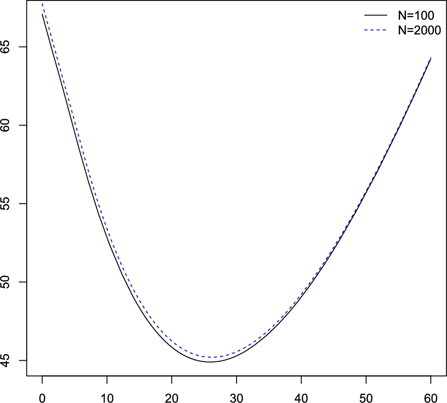
Denote by $u_{α, k}^{N} (\cdot)$ , $k \in N$ , the functions produced by the API algorithm with discount factor α when it is used a grid with N nodes and, similarly, the constant ${\tilde{S}}_{α, k}^{N}$ stands for the re-order point of the policy $g_{k}$ computed by the API algorithm with N nodes. The algorithm starts with the policy $g (x) : = 0$ , $x \in X$ , and stops once the quantity $‖ u_{k} - u_{k - 1} ‖_{\infty}$ falls below the tolerance $ε : = 0.001$ . Table 1 shows the numerical results for the API algorithm with discount factors $α = 0.6$ and $α = 0.99$ , and a grid with N nodes for $N = 100, 500, 1000, 2000$ .

Fig. 1.

Approximate policy iteration functions $u_{0.6, 4}^{N} (\cdot)$ for $N = 200, 2000$ .

Fig. 2.

Approximate policy iteration functions $u_{0.99, 4}^{N} (\cdot)$ for $N = 200, 500, 1000, 2000, 3000$ .

Table 1 and Figs 1 and 2 show that the API algorithm converges very fast and that practically identifies the optimal re-order point. In all these cases the API algorithm stops at the fourth iteration. In fact, $u_{α, 4}^{2000} (\cdot)$ is virtually the optimal value function $V^{*} (\cdot)$ and $S_{α, 5}$ is the optimal re-order point for $α = 0.6 and 0.99$ .

Table 2 below displays bounds for $δ_{C}$ and $δ_{Q}$ as well as for the performance errors $E_{1}$ and $E_{2}$ . Notice that $E_{1}$ and $E_{2}$ are very sensitive to the discount factor α even though the quantities $δ_{C}$ and $δ_{Q}$ can be controlled easily. In fact, the bounds $E_{1}$ and $E_{2}$ look quite conservative, specially if they are compared with the values given in Table 1. However, recall that (27) and (28) guarantee that $E_{1}$ and $E_{2}$ can be done arbitrarily small taking – perhaps unnecessarily – fine enough grids.

Table 2

Bounds for the performance errors $E_{1}$ and $E_{2}$ for an inventory systems with exponentially distributed demand with parameter $λ = 0.1$ and discount factor $α = 0.6$

	N

	100	500	1000	2000	5000	10,000
$δ_{C}$	2.8	0.56	0.28	0.14	0.056	0.028
$δ_{Q}$	0.48	0.096	0.048	0.024	0.0096	0.0048
$E_{1}$	97	19.4	9.7	4.75	1.93	0.95
$E_{2}$	194	38.8	19.4	9.5	3.86	1.9

Table 3

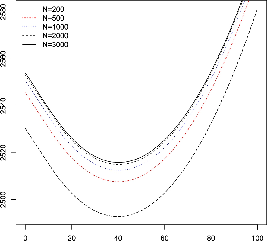
Approximate optimal policies produced by estimation–approximation policy iteration. The optimal re-order point are $S_{0.6}^{*} = 11.4663$ and $S_{0.99}^{*} = 15.79$

	$α = 0.6$ , $k = 4$			$α = 0.99$ , $k = 4$

t	10	20	50	10	20	50
$‖ u_{4} - u_{3} ‖$	6.064e ⁻⁷	5.984e ⁻⁷	7.331e ⁻⁷	3.526e ⁻⁵	2.050e ⁻⁵	3.084e ⁻⁵
${\tilde{S}}_{α, 4, t}$	13.9394	11.6970	11.5385	16.5738	16.0126	15.8759
$θ_{t}$	5.32533	5.23075	5.072251	5.783765	5.222557	5.0859

In the following consider the case in which the demand density function belongs to the parametric family of densities $\begin{matrix} (29) & ρ_{θ} (z) = λ exp (- λ (z - θ)) I_{[θ, \infty)} (z), \end{matrix}$ where the parameter θ is unknown but lies in some interval $Θ = [θ_{1}, θ_{2}]$ with $0 ⩽ θ_{1} < θ_{2}$ . Thus, the goal is to estimate the unknown parameter θ, and based on the estimate to compute approximated optimal policies. The maximum likelihood estimator of θ is $θ_{t} = min {w_{0}, w_{1}, \dots, w_{t - 1}}$ , so the density estimate is $\begin{matrix} (30) & ρ_{t} (z) = λ exp (- λ (z - θ_{t})) I_{[θ_{t}, \infty)} (z) . \end{matrix}$

The bounds for quantities $δ_{C^{(t)}}$ and $δ_{Q^{(t)}}$ defined in (14) and (15) can be obtained in a similar way as it was done for $δ_{C}$ and $δ_{Q}$ but using $ρ_{t} (\cdot)$ instead of $ρ (\cdot)$ after noting that density $ρ_{t} (\cdot)$ is bounded by $l_{t}^{'} : = λ$ and Lipschitz continuous with modulus $l_{t} = λ^{2} exp (λ θ_{t})$ . Thus, from (25) and (26), $\begin{matrix} \begin{matrix} δ_{C^{(t)}} ⩽ (p + 2 h + 2 c) Δ s and \\ δ_{Q^{(t)}} ⩽ (2 K l_{t} + 4 l_{t}^{'} M) Δ s, \end{matrix} \end{matrix}$ so, by Remarks 4.5(b) and 4.6 (see (18)), it holds that $\begin{array}{l} E {‖ {\tilde{V}}_{t}^{*} - V_{*} ‖}_{\infty} \\ ⩽ \frac{p + 2 h + 2 c}{1 - α} Δ s + \frac{α M (2 K l_{t} + 4 β_{t})}{{(1 - α)}^{2}} Δ s \\ (31) & + {\frac{M}{1 - α} + \frac{α M}{{(1 - α)}^{2}}} \frac{2}{(t + 1)} \end{array}$ and $\begin{array}{l} E ‖ V_{*} - V_{{\hat{g}}_{k}} ‖_{\infty} \\ ⩽ {\frac{p + 2 h + 2 c}{1 - α} + \frac{α M (2 K l_{t} + 4 β_{t})}{{(1 - α)}^{2}}} Δ s \\ + {\frac{M}{1 - α} + \frac{α M}{{(1 - α)}^{2}}} \frac{2}{(t + 1)} \\ (32) & + \frac{2 α}{1 - α} E ‖ v_{k} - v_{k - 1} ‖_{\infty}, \end{array}$ where $β_{t} : = E l_{t} = λ^{2} t e^{λ θ} {(t - 1)}^{- 1} ⩽ λ^{2} t e^{λ θ_{2}} {(t - 1)}^{- 1}$ .

The numerical results shown in Table 3 correspond to the values $c = 1.5$ , $h = 0.5$ , $p = 3$ , $K = 40$ , $λ = 0.1$ and discount factors $α = 0.6, 0.99$ . The EAPI algorithm was performed with samples $w = (w_{0}, \dots, w_{t - 1})$ simulated from the density (30) for $t = 10, 20, 50$ assuming that the true parameter value is $θ = 5$ and using a grid with $N = 100$ evenly spaced nodes.

Footnotes

Acknowledgements

Work supported partially by Consejo Nacional de Ciencia y Tecnologia (CONACyT) under Grant CB2015/254306 and also by Proyectos FEC-2015 de la División de Ciencias Exactasy Naturales, Universidad de Sonora.

The proof of Theorem 4.3 is based on Lemma A.1, Remark A.2 and Lemma A.3 given below.

Next it is the proof of Theorem 4.3.

References

Almudevar

, Approximate fixed point iteration with an application to infinite horizon Markov decision processes, SIAM Journal on Control and Optimization 46 (2008), 541–561.

Antos

Szepesvari

and Munos

, Learning near-optimal policies with Bellman-residual minimization based fitted policy iteration and a single sample path, Machine Learning 71 (2008), 89–129.

Bersetkas

D.P.

, Approximate policy iteration: A survey and some new methods, Journal of Control Theory and Applications 9 (2011), 310–335.

Bertsekas

D.P.

and Tsitsiklis

J.N.

, Neuro-Dynamic Programming, Athena Scientific, Belmont, MA, 1995.

Cooper

W.L.

Henderson

S.G.

and Lewis

M.E.

, Convergence of simulation-based policy iteration, Probability in the Engineering and Informational Sciences 17 (2003), 213–234.

Devroye

and Györfi

, Nonparametric Density Estimation: The L₁ View, Wiley, New York, 1985.

Devroye

and Lugosi

, Combinatorial Methods in Density Estimation, Springer, New York, 2001.

Farahmand

Ghavamzadeh

Szepesvari

and Mannor

, Regularized policy iteration, in: Advances in Neural Information Processing Systems, Vancouver, BC, Canada, 2008, pp. 441–448.

Gordienko

E.I.

and Minjárez-Sosa

J.A.

, Adaptive control for discrete-time Markov processes with unbounded costs: Discounted criterion, Kybernetika 34 (1998), 217–234.

10.

Hernández-Lerma

, Adaptive Markov Control Processes, Springer, New York, 1989.

11.

Hernández-Lerma

and Lasserre

J.B.

, Discrete-Time Markov Control Processes: Basic Optimality Criteria, Springer, New York, 1996.

12.

Hilgert

and Minjárez-Sosa

J.A.

, Adaptive policies for time-varying stochastic systems under discounted criterion, Math. Methods Oper. Res. 54 (2001), 491–505.

13.

Hilgert

and Minjárez-Sosa

J.A.

, Adaptive control of stochastic systems with unknown disturbance distribution: Discounted criteria, Math. Methods Oper. Res. 63 (2006), 443–460.

14.

and Powell

W.B.

, A convergent recursive least squares approximate policy iteration algorithm for multi-dimensional Markov decision process with continuous state and action spaces, in: IEEE Symposium on Adaptive Dynamic Programming and Reinforcement Learning, New York, 2009, pp. 66–73.

15.

and Powell

W.B.

, Convergence Analysis of Kernel-based On-policy Approximate Policy Iteration Algorithms for Markov Decision Processes with Continuous Multidimensional States and Actions, Department of Operations Research and Financial Engineering, Princeton University, 2010.

16.

Minjárez-Sosa

J.A.

, Approximation and estimation in Markov control processes under a discounted criterion, Kybernetika 40 (2004), 681–690.

17.

Munos

, Performance bounds in

L_{p}

-norm for approximate value iteration, SIAM Journal on Control and Optimization 47 (2007), 2303–2347.

18.

Powell

W.B.

, Approximate Dynamic Programming: Solving the Curse of Dimensionality, Wiley, 2007.

19.

Powell

W.B.

, Perspectives of approximate dynamic programming, Ann. Oper. Res. (2012), 1–38. doi:10.1007/s10479-012-1077-6.

20.

Powell

W.B.

and Ma

, A review of stochastic algorithms with continuous value function approximation and some new approximate policy iteration algorithms for multidimensional continuous applications, Journal of Control Theory and Applications 9 (2011), 336–352.

21.

Rieder

, Measurable selection theorems for optimization problems, Manuscripta Math. 24 (1978), 115–131.

22.

Rust

, Numerical dynamic programming in economics, in: Handbook of Computational Economics Amman

H.M.

Kendrick

D.A.

and Rust

, eds, Vol. 1, Elsevier, 1996, pp. 619–728.

23.

Rust

, A comparison of policy iteration methods for solving continuous-state, infinite-horizon Markovian decision problems using random, quasi-random, and deterministic discretization, available at SSRN: http://ssrn.com/abstract=37768 or https://dx-doi-org.web.bisu.edu.cn/10.2139/ssrn.37768.

24.

Santos

M.S.

and Rust

, Convergence properties of policy iteration, SIAM Journal on Control and Optimization 42 (2004), 2094–2115.

25.

Serfling

R.J.

, Approximation Theorems of Mathematical Statistics, Wiley, 2002.

26.

Stachurski

, Continuous state dynamic programming via nonexpansive approximation, Computational Economics 31 (2008), 141–160.

27.

Vega-Amaya

and López-Borbón

, A performance bound for discounted approximate dynamic programming using averagers, Reporte Interno, Departamento de Matemáticas, Universidad de Sonora, 2013.

28.

Vega-Amaya

and Montes-de-Oca

, Application of average dynamic programming to inventory systems, Math. Methods Oper. Res. 47 (1998), 451–471.

29.

and Lu

, Kernel-based least squares policy iteration for reinforcement learning, IEEE Transactions on Neural Networks 18 (2007), 973–992.