The idiosyncratic volatility puzzle and mergers and acquisitions activity

Abstract

This paper examines whether the puzzling negative relationship between idiosyncratic volatility and next month performance is affected by the intensity of merger and acquisition (M&A) activity in the market. Our results show that the idiosyncratic volatility puzzle is stronger in periods of high M&A activity than in periods of low M&A activity. Further analysis shows that the negative relationship between idiosyncratic volatility and next month performance is the strongest in the high M&A activity sub-period spanning from 1982–1989. In contrast, M&A activity does not explain the negative relationship between the common factor in idiosyncratic volatility (CIV) and next month performance. M&A activity can in part explain the idiosyncratic volatility puzzle, but it does not subsume the negative relationship between CIV exposure and firm returns.

Keywords

Idiosyncratic Volatility mergers and acquisitions activity merger and acquisition waves volatility trends expected returns asset pricing multifactor models

1. Introduction

There is an extensive empirical literature analyzing the relationship between idiosyncratic volatility and stock returns. The signals emanating from this literature are diverse if not to say mixed; they vary depending on the model used to estimate idiosyncratic volatility, the frequency of the returns data used to estimate idiosyncratic volatility, and whether or not microstructure noise or return reversals are controlled for. This paper offers a new perspective to the debate regarding one of the most prominent regularities identified: the puzzling negative relationship between idiosyncratic volatility and subsequent month performance as documented by Ang et al. [2]. Specifically, in this paper we test whether this puzzle is related to mergers and acquisitions (M&A hereafter) activity. The M&A literature suggest that a nationwide M&A wave is a clustering of a series of M&A waves in different industries (e.g. Ahern and Harford [1]). This clustering is boosted or facilitated by liquidity and misvaluation. The industry waves themselves are usually initiated by internal shocks that are usually the results of technological changes in the corresponding industry. Both industry internal shocks and market misvaluation create uncertainty related to the future prospects of firms that are varying from industry to another and from one company to another within the same industry according to the exposure of this company to its new operating environment. In addition, a company involved in an M&A deal would passes through a period of instability related to its own future prospects as the deal is negotiated and in the transitional period over which visions, cultures and operations are combined under one management. Finally, that acquisitions initiated during merger have been shown to be associated with poorer quality of analysts’ forecasts, greater uncertainty and weaker CEO turnover-performance sensitivity, leading to inferior monitoring and inefficient mergers (Duchin and Schmidt [15]). We hypothesize that these sources of uncertainty about the firm’s future prospects should be incorporated into the firm’s actual idiosyncratic volatility and will influence the observed relationship between measured idiosyncratic volatility and next month expected returns.

Our findings are consistent with this hypothesis. Specifically, we find that the idiosyncratic volatility puzzle documented by Ang et al. [2] is related to M&A activity: the negative relationship between idiosyncratic volatility and subsequent month returns is considerably stronger in periods of high M&A activity than in periods of low M&A activity, with the greatest impact observed during the intense M&A wave spanning the period 1982–1989: the observed trends in both alphas and returns decrease systematically while moving from the lowest to the highest idiosyncratic volatility quintile in addition to the significant negative performance of the zero investment portfolio that is long the high idiosyncratic volatility quintile (Q5) and short the low idiosyncratic volatility quintile (Q1). It seems that M&A activities are amplifying the uncertainties surrounding the firms (bidders and targets) future prospects. These uncertainties are transmitted to higher firm specific volatilities. When the number of such firms increases during a specific period of time, their effect gets into the relationship between idiosyncratic volatility and next month performance touching the well-known idiosyncratic volatility puzzle. In a recent paper, Bhagwat, Dam and Harford [7] show that an increase in aggregate market volatility will lead to a decrease in the following month deal activities. They explain this link by saying that the high VIX will drive the volatility of the high beta target firms leading to more uncertainty about these firms while negotiating the deal. The higher this uncertainty, the lower the deal activities.

In another recent paper, Herskovic et al. [23] show that shocks to the common idiosyncratic volatility factor (CIV) are priced and that stocks with lower CIV-exposure in a particular month perform better than their higher CIV-exposure peers in the next month. They attribute this result to household utility effects arising from cross sectional volatility in consumption growth. Our paper test whether the CIV exposure effect may be a consequence of perceived volatility of firm prospects arising from changes in the market for corporate control. Specifically, we test whether the CIV exposure effect is persistent across periods of high and low mergers and acquisitions activities. Our motives to investigate such a relationship between mergers’ activities and the exposure to the common idiosyncratic volatility factor is driven by the economy wide uncertainty which may give rise to mispricing at the firm level. Consistent with Herskovic et al. [23], we find that firms with higher exposure to the CIV factor exhibit lower future returns. However, in contest with the negative relationship between idiosyncratic volatility and M&A activity, this relationship is not affected by M&A activity. In other words, economy-wide uncertainty as reflected in the CIV factor is not significantly influenced by M&A activity. M&A activity can in part explain the idiosyncratic volatility puzzle, but it does not subsume the negative relationship between CIV exposure and firm returns.

The remainder of the paper proceeds as follows. In Section 2 we provide a brief review of the relevant literature, and introduce our hypotheses. Section 3 describes our data and methodology. The empirical results follow in Sections 4 to 7. The paper concludes with a summary in Section 8.

2. Literature review

2.1. Firm level idiosyncratic volatility and stock returns

Ang et al. [2] find that stocks with higher idiosyncratic volatility have lower returns. This result is puzzling, in that conventional theory suggests that idiosyncratic volatility should not be priced as it is diversifiable. If idiosyncratic volatility cannot be diversified away, then investors would demand compensation for bearing the idiosyncratic risk and this should be translated into stock with higher idiosyncratic volatility associated with higher returns. More recent theoretical extensions have looked at the effects of risk tolerance, information (firm visibility), transactions costs, and short selling constraints in establishing a premium for idiosyncratic volatility (e.g. Levy [31], Merton [35], Jones and Rhodes-Kropf [27], and Malkiel and Xu [33], and Boehme, Danielsen, Kumar and Sorescu [9]. These papers show that stocks that face short-sale constraints and belong to less visible firms exhibit a positive relationship between expected returns and idiosyncratic volatility). Ang et al. [3] find that the idiosyncratic volatility effect is not limited to the USA: it is also observed for other G7 countries.

A considerable body of work has emerged that addresses this puzzle as a model based problem and/or a returns distribution problem. Brockman and Schutte [10] show that using an EGARCH to model expected idiosyncratic volatility would lead to a positive relationship between idiosyncratic volatility and stock returns in the international market. They attribute the negative relationship to the use of the previous month’s idiosyncratic volatility as a proxy to next month expected volatility. Fu [18] argues in this vein and in line with Huang, Liu, Rhee and Zhang [25], shows that return reversal of stocks with high idiosyncratic volatility also plays a role. More specifically, stocks with high idiosyncratic volatility may exhibit high contemporaneous returns. The positive abnormal returns tend to reverse, resulting in negative abnormal returns in the following month. From this perspective, the negative relationship found between idiosyncratic volatility and expected stock returns maybe explained by two combined effects: the negative serial correlation in monthly returns of individual stocks and the positive contemporaneous relation between realized monthly idiosyncratic volatility and stock returns. Spiegel and Wang [41] show that idiosyncratic volatility and stock liquidity are negatively correlated. In addition, they demonstrate that stocks are decreasing in liquidity and increasing in idiosyncratic volatility and that the idiosyncratic volatility effect dominates the liquidity effect when tested together. In contrast to Ang et al. [2] they use monthly return observations rather than daily returns observations in estimating their idiosyncratic volatility. They also test the contemporaneous relationship between idiosyncratic volatility and returns and not a lead-lag relationship as in Ang et al. [2]. Bali and Cakici [5] show that if only stocks listed on NYSE are used to create the portfolio quintiles cut-off point, (in line with Fama and French ‘1993’ portfolio creation approach), rather than the entire CRSP universe, then the relationship between idiosyncratic volatility and stock expected returns becomes insignificant. In addition, forming equally weighted portfolios instead of value-weighted portfolio dilutes the significance of puzzle. Finally, they demonstrate that the negative relationship between idiosyncratic volatility and expected stock returns is not significant, when monthly data instead of intra month daily data are used to estimate idiosyncratic volatility. Boehme, Danielsen, Kumar and Sorescu [9] show that stocks that face short-sale constraints and belong to less visible firms exhibit a positive relationship between expected returns and idiosyncratic volatility. Switzer and Picard [42] incorporate momentum and liquidity into the Fama and French [16] three factor model to estimate idiosyncratic volatility. They found no idiosyncratic volatility effect for developed markets using this model.

Another branch of literature links the idiosyncratic volatility puzzle to market imperfections and microstructure noise. Han and Lesmond [21] argue that the idiosyncratic volatility puzzle diminishes if we use the quoted mid-point based returns instead of using the closing price returns. They interpret their result by explaining that the mid-point quoted prices would correct for microstructure noise (bid-ask bounce) argued by Blume and Stambaugh [8]. Jiang, Xu and Yao [26] link the idiosyncratic volatility puzzle to earning shocks and firm visibility. They show that idiosyncratic volatility is inversely related to expected earnings and earning shocks. This relationship between idiosyncratic volatility and expected earning is inducing the negative relationship observed between idiosyncratic volatility and expected returns. In other words, controlling for earning shocks would remove the significance of the negative relationship between idiosyncratic volatility and expected returns. In addition, they also link the relationship between idiosyncratic volatility and expected earning to selective corporate disclosure practices; corporate selective disclosure. This link is more robust for firms with less sophisticated investors. Chen and Petkova [11] associate the idiosyncratic volatility puzzle with a missing systematic risk factor in the Fama–French model. They show that portfolios with high idiosyncratic volatility have positive exposure to innovations in the average stock variances and consequently they have a lower expected returns. More recently, Hou and Loh [24] try to measure how much of the idiosyncratic volatility puzzle is explained by market frictions factors (including return reversals, bid-ask spread, Amihud illiquidity, clustered zero-return observations), investors preferences for lottery stocks (exhibiting skewness, co- skewness, maximum daily return) and other factors including earnings surprises. They find that while much of the idiosyncratic volatility puzzle is explained by the previously mentioned factors, a significant portion of the puzzle remains unexplained.

Our work sheds new light one firm level idiosyncratic volatility puzzle in two ways. First we show that the idiosyncratic volatility puzzle is stronger in high M&A activity periods than in low M&A activity periods. This result is consistent with the existence of a spillover effect from the uncertainty about the future prospects of companies (target and acquirer) involved in an M&A deal to the firm specific uncertainty that is incorporated into the firms’ idiosyncratic volatility. Second we show that using daily or monthly returns in the performance estimation window and Fama and French [16] three factors model or Fama and French [17] five factor model affects the robustness of the puzzle across our total sample but does not mitigate our basic result that the negative relationship between idiosyncratic volatility and next month’s performance is clustered in periods of high M&A activity relative to periods of low M&A activity.

2.2. Aggregate idiosyncratic volatility, common factor idiosyncratic volatility and stock returns

A related branch of literature assesses the effect of aggregate idiosyncratic volatility as a risk factor on stock returns. Goyal and Santa-Clara [19] report that the equal-weighted total volatility is positively and significantly related to future stock market returns, although stock market volatility is not. Guo and Savickas [20] show that idiosyncratic volatility has predictive power over aggregate stock market returns. They also show that the aggregate idiosyncratic volatility and aggregate B/M ratio are significantly negatively correlated and that the idiosyncratic volatility factor explain the cross-section of stock returns as well as the B/M ratio when tested on the 25 Fama and French [16] portfolios. Duarte, Kamara, Siegle and Sun [14] show that the pricing of aggregate idiosyncratic volatility is due to unaccounted systematic risk factor. They call their factor Predicted Idiosyncratic Volatility (PIV). They show that the first common idiosyncratic volatility component is significantly correlated with business cycle variables such as default spread as well as average stock volatility. They constructed a PIV risk factor in the footsteps of Fama and French [16] factors by obtaining the difference between the return on a portfolio of stocks in the highest quintile of predicted idiosyncratic volatility and the return on a portfolio of the stocks in the lowest quintile of predicted idiosyncratic volatility. Their PIV explains the excess return of the 30 Fama and French [16] industry portfolios and is priced even in the presence of momentum and liquidity factor. Herskovic, Kelly, Lustig and Van Nieuwerburgh [23] show that the firm-level idiosyncratic volatilities possess a high degree of comovement that is described by a factor model, they called it common factor in idiosyncratic volatility (CIV). They show that CIV is correlated to idiosyncratic income risk. They estimate their CIV as equal-weighted average of market model residuals. They show that average returns are decreasing with CIV beta exposures: firms that have a more positive exposure to CIV innovations earn lower average returns. Their results is robust after accounting for Pastor-Stambaugh liquidity measure. In this paper, we test whether the results found by Herskovic et al. [23] are driven by model specification as well as by M&A activities.

2.3. Linking takeover waves to idiosyncratic volatility

As defined in Betton, Eckbo and Thorburn [6]: “A merger wave is a clustering in time of successful takeovers bids at the industry or economy wide level.” In this paper we focus our analysis on economy wide clustering of merger activities. There are two main hypotheses that compete in explaining merger waves: the neoclassical hypothesis pioneered by Lang et al. [30] and Servaes [39] and the inefficient markets hypothesis of Shleifer and Vishny [40] and Rhodes-Kropf and Viswanathan [38]. Under the neoclassical hypothesis, merger waves are preceded by technological, regulatory, and economic shocks in the industry in which the wave is occurring. Managers, reacting to these shocks, engage in M&A activity in their attempt to compete for the optimal asset combination. Under the inefficient markets hypothesis, market misvaluation is the main driver of merger waves.

Lang, Stulz and Walking [30] study tender offers in an efficient markets neoclassical framework, using Tobin’s Q as a proxy for management skill. They find that takeovers of poorly managed targets (low Tobin’s Q) by better managed bidders (high Tobin’s Q) have higher bidder, target, and total (bidder plus target) gains. Servaes [39] extends the analyses of Lang, Stulz and Walking [30] by covering both mergers and tender offers. He shows that targets’, bidders’ and total returns are larger when targets have low Tobin’s Q ratios and bidders have high Tobin’s Q ratios. This finding is consistent with the argument that value is created when well managed bidders overtake poorly managed targets. Mitchell and Mulherin [36] show that takeover activities in the 1980’s are clustered in industries that experience fundamental shocks to technology, government policies, and demand and supply conditions, which is also consistent with the efficient markets neoclassical framework. Jovanovic and Rousseau [29] contend that the merger waves of the 1900 and the 1920’s, ’80s, and ’90s were a response to profitable reallocation opportunities, in contrast to the ’60s wave which remains unexplained. Harford [22] presents evidence in support of the neoclassical hypothesis with minor modifications: industry shocks would lead to merger waves in a particular industry only when there is enough liquidity to accommodate the reallocation of asset. Thus industry merger activities may have to wait until enough liquidity is present in the market. Consequently, industry merger waves may cluster leading to an aggregate economy wide merger waves.

Shleifer and Vishny [40] assume that financial markets are inefficient, leading to firm mispricing. Rational managers seek to exploit this mispricing by acquiring less valued targets through stock rather than cash acquisitions. Shleifer and Vishny [40] show that merger activities coincide with higher market valuations, similar to Maksimovic and Phillips [32] and Jovanovic and Rousseau [28]. Their findings are consistent with the inefficient markets approach. Dong et al. [13] find that more highly valued bidders are more likely to use stock, less likely to use cash, willing to pay more relative to target market price and earn lower announcement period returns. Rhodes-Kropf, Robinson and Viswanathan [37] decompose the M/B ratio into three components: the firm specific pricing deviation from short-run industry pricing; the short-run deviations from firms’ long-run pricing; and the long-run pricing to book, which serves as a proxy for the firm’s growth potential. Based on this decomposition, they uncover several relevant findings: the large difference in the target and acquirer M/B is mainly driven by the higher firm specific error in the acquirer M/B. The target M/B has a minimal portion of firm specific error. They also demonstrate that acquirers and targets cluster in sectors with high time-series sector error. They both have a common misvaluation component in their M/B. It seems that overvalued firms buy less overvalued firms that are by themselves overvalued. In addition, firms with higher firm specific error are more likely to become acquirers of firms with transactions that are financed by stock issuance. These results suggest that although economic shocks maybe driving merger activities in an industry, misvaluation plays an important role in determining who buys whom. Ang and Cheng [4] show that acquirers are more overvalued in successful stock mergers than in withdrawn mergers. They also find that the probability of a firm becoming a stock acquirer increases with its overvaluation. In addition, they show that if the acquirer level of overvaluation is greater than the premium adjusted overvaluation, then the acquirer firms are better off than their non-merged peers, consistent with positive synergy in mergers.

Mitchell and Mulherin [36] allude to industry shocks as drivers of merger waves, such as monopoly creation as the main driver of the 1890s merger wave, oligopoly creation for the 1920s merger wave, conglomerate diversification for 1960s merger wave, break-down of the 1960’s conglomerate cohort for the 1980s merger wave, and deregulation for the 1990s wave. More recently, Duchin and Schmidt [15] demonstrate that acquisitions initiated during industry specific merger waves, are associated with poorer quality of analysts’ forecasts, greater uncertainty, and weaker CEO turnover-performance sensitivity. These factors inhibit monitoring, giving rise to more inefficient mergers. We hypothesize that shocks’ propagation and misvaluations would find their way into the firm level idiosyncratic volatility if they don’t span the whole economy, the market as well as the risk factors’ inherent in the model used as a benchmark in the estimation of the firm’s expected returns. In other words, we expect that merger waves should impact directly on the estimation of idiosyncratic volatility per se, and in turn on the robustness of the idiosyncratic volatility puzzle.

We propose to test for the first time the mergers wave effect as a driver of idiosyncratic volatility shocks that systematically affect stock returns.

Hypothesis 1.
M&A waves are associated with increased misvaluations that are due to increased uncertainty about the firm’s future prospects that are incorporated into the firm’s actual idiosyncratic volatility. This will influence the observed relationship between measured idiosyncratic volatility and next month expected returns. As a consequence, the idiosyncratic volatility puzzle is stronger in periods of high M&A activity than in periods of low M&A activity.
Hypothesis 2.
The negative relationship between CIV exposure and firm returns is related to changes in uncertainties in firms’ opportunity sets, including uncertainties in marginal returns investment associated with M&A waves.

3. Data and methodology

The sample for our study spans the period 1960–2013. Harford [22] analyzes two aggregate merger waves in the 1980s and 1990s: one spanning from 1986 to 1988 and another spanning from 1996 to 1999. Martynova and Renneboog [34] identify five merger waves in the US as: wave 1 (1890s–1903), wave 2 (1910s–1929), wave 3 (1950s–1973), wave 4 (1981–1989), wave 5 (1993–2001). Ahern and Harford’s [1] (2003–2008) merger wave overlaps with Martynova and Renneboog [34] sixth merger wave. Our analyses cover the following five merger wave periods from 1960–2013: Wave A (1960–1972), Wave B (1982–1989), Wave C (1993–2000), Wave D (2004–2007), and Wave E (2013); the latter represents the onset of the most recent merger wave, based on Mergerstat.1 The corresponding periods of no merger wave (‘1973–1981’, ‘1990–1992’, ‘2001–2003’, ‘2008–2012’) as those with low mergers and acquisitions activity.

Stock price and return data are obtained from CRSP covering stocks listed on NYSE, NYSE MKT (formerly AMEX), and NASDAQ. Consistent with the previous literature, we have removed ETFs. Closed End Funds, and REITS from our sample,

Our initial benchmark for testing the effect of lagged monthly idiosyncratic volatility on monthly performance uses the Ang et al. [2] specification. We divide our sample period between periods with high M&A activity versus period with low M&A activity. Idiosyncratic volatility is measured as the realized volatility of the residuals obtained after estimating the Fama and French [16] three-factor model. Using daily data, for each stock in our sample, for every month, we estimate the Fama–French [16] three factor model: $\begin{matrix} (1) & \begin{matrix} r_{i, t} - R_{f, t} \\ = α_{i} + β_{MKT, i} (R_{m, t} - R_{f, t}) \\ + β_{SMB, i} {SMB}_{t} + β_{HML, i} {HML}_{t} + ϵ_{t} . \end{matrix} \end{matrix}$ $r_{i, t} - R_{f, t}$ corresponds to the excess daily return of stock i on day t, $α_{i}$ is the Fama–French adjusted alpha, $R_{m, t} - R_{f, t}$ , ${SMB}_{t}$ , ${HML}_{t}$ correspond to the market risk premium, small cap premium factor and the value premium factor respectively

As complementary tests, we estimate the idiosyncratic volatility using the Fama and French [17] five factor model: $\begin{matrix} (2) & \begin{matrix} r_{i, t} - R_{f, t} \\ = α_{i} + β_{MKT, i} (R_{m, t} - R_{f, t}) + β_{SMB, i} {SMB}_{t} \\ + β_{HML, i} {HML}_{t} + β_{RMW, i} {RMW}_{t} \\ + β_{CMA, i} {CMA}_{t} + ϵ_{t} \end{matrix} \end{matrix}$ where $R_{m, t} - R_{f, t}$ , ${SMB}_{t}$ , ${HML}_{t}$ are as defined as in (1), ${RMW}_{t}$ is the difference between the returns on a diversified portfolios of stocks with robust and weak profitability, and ${CMA}_{t}$ is the difference between the returns on diversified portfolios of stocks with low and high investment firms. As such, RMW and CMA would proxy for profitability and investment respectively. We estimate the idiosyncratic volatility for the Fama and French [17] model in exactly the same way we did for the Fama and French [16] model. In addition, once stocks are sorted into quintiles based on their respective lagged idiosyncratic volatility, value-weighted portfolios are formed and their Five-Factor Alpha as well as their average returns are estimated. The Fama and French [16,17] factors are downloaded from Kenneth French’s webpage.

Once idiosyncratic volatilities are estimated, stocks are sorted into quintile portfolios based on their idiosyncratic volatility. The quintile portfolios are value-weighted, formed at the beginning of the month and kept for one month. The process is repeated recursively on monthly basis and we end out having five quintile portfolios with value-weighted daily returns.

Next we estimate the Fama and French [16] adjusted alpha for these portfolios as well as the average returns of these portfolios over our total sample period, high M&A activity sub-periods and low M&A activities sub-period. For a firm monthly idiosyncratic volatility to be included in our sample, we require the presence of at least 12 daily observations within the idiosyncratic volatility estimation month; otherwise the stock’s monthly observation is dropped out from our sample and consequently it is not included in forming next month quintile portfolios.

We also estimate the performance of the portfolios using monthly returns for comparative purposes.

4. Trends in aggregate volatilities

Table 1 presents summary statistics (mean and standard deviation) of the monthly returns of all the stocks in our sample per year of observation as well as the number of stocks in the sample for each year. We also report the average monthly idiosyncratic volatilities estimated using daily returns using the Fama–French three-factor model. In addition, we report the ratios of idiosyncratic volatility to total volatility. Panel A reports the estimates using equal-weighted idiosyncratic volatility. Panel B shows the results using value weighted idiosyncratic volatility. As can be seen therein, there is considerable variation through time of the volatility measures. There is some secular decline in the number of stocks in the sample each year since 1999.

Considerable volatility spikes are observed for the OPEC Oil Crisis period 1973–74, for the stock market crash year of 1987, and the Russian Default and Long term Capital Management Crises of 1998; peak volatilities for the sample are observed during the Great Financial Crisis of 2008–9.

Table 1
In the table we provide the average statistics for our sample. The monthly return is obtained every month for every firm in our sample. Then equal (value) weighted average for all firm’s return is obtained. The reported returns are then averaged for the 12 months within every year to obtain our yearly observations. The idiosyncratic volatility is estimated every month for every firm relative to the Fama and French [16] three factor model using the daily returns within this month. Then, equal (value) weighted average for all firm’s idiosyncratic volatility is obtained. The reported idiosyncratic volatilities are then averaged for the 12 months within every year to obtain our yearly observations. The return’s volatility is estimated every month for every firm using the daily returns within this month. Then, equal (value) weighted average for all firm’s return’s volatility is obtained. Then, equal (value) weighted average for all firm’s volatility is obtained. The reported volatilities are then averaged for the 12 months within every year to obtain our yearly observations. Scaled Idiosyncratic Volatility is obtained by dividing the monthly aggregate idiosyncratic volatility by the monthly aggregate return volatility. The reported scaled idiosyncratic volatilities are then averaged for the 12 months within every year to obtain our yearly observations. The number of stocks per year is the total number of firms that are used within any month during this year (each firm is counted once within any year)

Year Average Monthly Return Average Firms’ Volatility Average Firms’ Idiosyncratic Volatility Average Firms’ Scaled Idiosyncratic Volatility Number of Stocks per Year Year Average Monthly Return Average Firms’ Volatility Average Firms’ Idiosyncratic Volatility Average Firms’ Scaled Idiosyncratic Volatility Number of Stocks per Year

Panel A – Descriptive Statistics – Equal-Weighted Volatility, Idiosyncratic Volatility, and Scaled Volatility

1963 0.28% 2.24% 2.13% 95.55% 2073 1989 0.90% 3.14% 3.09% 98.25% 6723

1964 1.42% 2.12% 2.09% 98.63% 2155 1990 −1.98% 4.01% 3.91% 97.67% 6547

1965 2.66% 2.17% 2.10% 96.90% 2208 1991 3.78% 4.22% 4.14% 98.18% 6514

1966 −0.44% 2.44% 2.26% 92.91% 2229 1992 2.29% 4.44% 4.39% 98.84% 6699

1967 5.06% 2.46% 2.36% 96.10% 2271 1993 2.00% 4.22% 4.20% 99.32% 7058

1968 3.09% 2.46% 2.33% 94.79% 2293 1994 −0.38% 4.01% 3.95% 98.55% 7529

1969 −2.25% 2.35% 2.18% 92.81% 2361 1995 2.38% 3.93% 3.89% 99.14% 7864

1970 −0.65% 2.97% 2.68% 91.11% 2430 1996 1.45% 3.88% 3.80% 98.11% 8396

1971 1.73% 2.53% 2.38% 94.20% 2516 1997 1.69% 3.88% 3.77% 97.29% 8621

1972 0.49% 2.35% 2.27% 96.57% 2649 1998 0.02% 4.45% 4.28% 96.39% 8441

1973 −3.46% 2.98% 2.81% 94.76% 5697 1999 2.76% 4.43% 4.34% 97.93% 8093

1974 −2.21% 3.25% 3.07% 94.47% 5115 2000 −0.91% 5.27% 4.99% 94.92% 7737

1975 4.63% 3.04% 2.92% 96.09% 4922 2001 2.37% 4.80% 4.52% 94.41% 6989

1976 3.64% 2.53% 2.46% 97.05% 4993 2002 −0.89% 4.31% 4.03% 93.69% 6265

1977 1.83% 2.20% 2.15% 97.56% 4974 2003 5.12% 3.30% 3.10% 93.90% 5814

1978 2.26% 2.44% 2.29% 94.36% 4931 2004 1.79% 2.76% 2.56% 92.70% 5631

1979 3.07% 2.37% 2.26% 95.29% 4875 2005 0.44% 2.54% 2.37% 93.44% 5604

1980 3.30% 2.70% 2.50% 93.24% 5048 2006 1.40% 2.46% 2.28% 92.66% 5527

1981 0.09% 2.55% 2.40% 94.36% 5416 2007 −0.40% 2.66% 2.39% 90.42% 5518

1982 1.97% 2.77% 2.63% 94.96% 5647 2008 −4.64% 4.93% 4.16% 86.32% 5220

1983 2.86% 2.73% 2.63% 96.34% 6228 2009 4.91% 4.71% 4.09% 87.63% 4893

1984 −1.00% 2.60% 2.51% 96.57% 6523 2010 2.33% 2.98% 2.57% 86.79% 4715

1985 2.00% 2.77% 2.72% 98.15% 6578 2011 −0.85% 3.15% 2.54% 82.71% 4568

1986 0.69% 3.05% 2.97% 97.54% 6876 2012 1.50% 2.68% 2.42% 90.28% 4414

1987 −0.31% 3.65% 3.39% 94.97% 7082 2013 3.07% 2.41% 2.20% 91.55% 4397

1988 1.53% 3.28% 3.20% 97.69% 7040 Total Sample 1.23% 3.20% 3.02% 94.78% 24644

Panel B – Descriptive Statistics – Value-Weighted Volatility, Idiosyncratic Volatility, and Scaled Volatility

1963 1.63% 1.23% 1.01% 85.13% 2073 1989 2.63% 1.49% 1.26% 85.53% 6723

1964 1.49% 1.05% 0.97% 92.95% 2155 1990 0.21% 1.79% 1.47% 83.41% 6547

1965 1.42% 1.11% 1.01% 91.11% 2208 1991 3.17% 1.81% 1.54% 85.39% 6514

1966 −0.30% 1.53% 1.29% 85.13% 2229 1992 1.31% 1.68% 1.52% 90.71% 6699

1967 2.62% 1.47% 1.34% 91.42% 2271 1993 1.53% 1.74% 1.59% 92.10% 7058

1968 1.65% 1.60% 1.45% 90.65% 2293 1994 0.53% 1.69% 1.54% 91.09% 7529

1969 −0.45% 1.56% 1.37% 87.96% 2361 1995 3.21% 1.66% 1.54% 92.72% 7864

1970 0.71% 1.86% 1.53% 83.77% 2430 1996 2.35% 1.84% 1.63% 89.09% 8396

1971 1.73% 1.50% 1.32% 88.58% 2516 1997 3.11% 2.05% 1.69% 82.92% 8621

1972 1.77% 1.39% 1.25% 90.37% 2649 1998 3.01% 2.40% 1.99% 84.26% 8441

1973 −0.93% 1.89% 1.56% 83.17% 5697 1999 3.76% 2.70% 2.32% 86.06% 8093

1974 −1.68% 2.28% 1.79% 79.13% 5115 2000 1.91% 3.68% 3.09% 84.66% 7737

1975 3.52% 1.89% 1.58% 83.74% 4922 2001 0.71% 2.76% 2.19% 80.32% 6989

1976 2.50% 1.44% 1.24% 85.94% 4993 2002 −0.75% 2.55% 1.93% 76.45% 6265

1977 0.10% 1.25% 1.09% 87.38% 4974 2003 3.05% 1.79% 1.38% 78.33% 5814

1978 1.26% 1.50% 1.23% 83.05% 4931 2004 1.50% 1.48% 1.23% 83.05% 5631

1979 2.39% 1.48% 1.26% 85.55% 4875 2005 1.07% 1.41% 1.18% 83.80% 5604

1980 3.45% 2.04% 1.67% 82.06% 5048 2006 1.70% 1.46% 1.23% 85.05% 5527

1981 0.48% 1.86% 1.58% 84.90% 5416 2007 1.15% 1.65% 1.26% 77.56% 5518

1982 2.39% 2.00% 1.62% 81.80% 5647 2008 −2.47% 3.30% 2.16% 69.49% 5220

1983 2.45% 1.81% 1.57% 87.25% 6228 2009 3.58% 2.58% 1.81% 71.82% 4893

1984 0.89% 1.66% 1.42% 85.43% 6523 2010 2.00% 1.72% 1.20% 71.60% 4715

1985 2.88% 1.51% 1.34% 88.88% 6578 2011 0.51% 1.96% 1.25% 67.71% 4568

1986 1.94% 1.77% 1.51% 85.82% 6876 2012 1.73% 1.47% 1.13% 77.22% 4414

1987 1.26% 2.34% 1.70% 79.21% 7082 2013 2.81% 1.35% 1.08% 80.78% 4397

1988 1.92% 1.70% 1.36% 81.23% 7040 Total Sample 1.58% 1.82% 1.50% 83.96% 24644

Year	Average Monthly Return	Average Firms’ Volatility	Average Firms’ Idiosyncratic Volatility	Average Firms’ Scaled Idiosyncratic Volatility	Number of Stocks per Year	Year	Average Monthly Return	Average Firms’ Volatility	Average Firms’ Idiosyncratic Volatility	Average Firms’ Scaled Idiosyncratic Volatility	Number of Stocks per Year
Panel A – Descriptive Statistics – Equal-Weighted Volatility, Idiosyncratic Volatility, and Scaled Volatility
1963	0.28%	2.24%	2.13%	95.55%	2073	1989	0.90%	3.14%	3.09%	98.25%	6723
1964	1.42%	2.12%	2.09%	98.63%	2155	1990	−1.98%	4.01%	3.91%	97.67%	6547
1965	2.66%	2.17%	2.10%	96.90%	2208	1991	3.78%	4.22%	4.14%	98.18%	6514
1966	−0.44%	2.44%	2.26%	92.91%	2229	1992	2.29%	4.44%	4.39%	98.84%	6699
1967	5.06%	2.46%	2.36%	96.10%	2271	1993	2.00%	4.22%	4.20%	99.32%	7058
1968	3.09%	2.46%	2.33%	94.79%	2293	1994	−0.38%	4.01%	3.95%	98.55%	7529
1969	−2.25%	2.35%	2.18%	92.81%	2361	1995	2.38%	3.93%	3.89%	99.14%	7864
1970	−0.65%	2.97%	2.68%	91.11%	2430	1996	1.45%	3.88%	3.80%	98.11%	8396
1971	1.73%	2.53%	2.38%	94.20%	2516	1997	1.69%	3.88%	3.77%	97.29%	8621
1972	0.49%	2.35%	2.27%	96.57%	2649	1998	0.02%	4.45%	4.28%	96.39%	8441
1973	−3.46%	2.98%	2.81%	94.76%	5697	1999	2.76%	4.43%	4.34%	97.93%	8093
1974	−2.21%	3.25%	3.07%	94.47%	5115	2000	−0.91%	5.27%	4.99%	94.92%	7737
1975	4.63%	3.04%	2.92%	96.09%	4922	2001	2.37%	4.80%	4.52%	94.41%	6989
1976	3.64%	2.53%	2.46%	97.05%	4993	2002	−0.89%	4.31%	4.03%	93.69%	6265
1977	1.83%	2.20%	2.15%	97.56%	4974	2003	5.12%	3.30%	3.10%	93.90%	5814
1978	2.26%	2.44%	2.29%	94.36%	4931	2004	1.79%	2.76%	2.56%	92.70%	5631
1979	3.07%	2.37%	2.26%	95.29%	4875	2005	0.44%	2.54%	2.37%	93.44%	5604
1980	3.30%	2.70%	2.50%	93.24%	5048	2006	1.40%	2.46%	2.28%	92.66%	5527
1981	0.09%	2.55%	2.40%	94.36%	5416	2007	−0.40%	2.66%	2.39%	90.42%	5518
1982	1.97%	2.77%	2.63%	94.96%	5647	2008	−4.64%	4.93%	4.16%	86.32%	5220
1983	2.86%	2.73%	2.63%	96.34%	6228	2009	4.91%	4.71%	4.09%	87.63%	4893
1984	−1.00%	2.60%	2.51%	96.57%	6523	2010	2.33%	2.98%	2.57%	86.79%	4715
1985	2.00%	2.77%	2.72%	98.15%	6578	2011	−0.85%	3.15%	2.54%	82.71%	4568
1986	0.69%	3.05%	2.97%	97.54%	6876	2012	1.50%	2.68%	2.42%	90.28%	4414
1987	−0.31%	3.65%	3.39%	94.97%	7082	2013	3.07%	2.41%	2.20%	91.55%	4397
1988	1.53%	3.28%	3.20%	97.69%	7040	Total Sample	1.23%	3.20%	3.02%	94.78%	24644
Panel B – Descriptive Statistics – Value-Weighted Volatility, Idiosyncratic Volatility, and Scaled Volatility
1963	1.63%	1.23%	1.01%	85.13%	2073	1989	2.63%	1.49%	1.26%	85.53%	6723
1964	1.49%	1.05%	0.97%	92.95%	2155	1990	0.21%	1.79%	1.47%	83.41%	6547
1965	1.42%	1.11%	1.01%	91.11%	2208	1991	3.17%	1.81%	1.54%	85.39%	6514
1966	−0.30%	1.53%	1.29%	85.13%	2229	1992	1.31%	1.68%	1.52%	90.71%	6699
1967	2.62%	1.47%	1.34%	91.42%	2271	1993	1.53%	1.74%	1.59%	92.10%	7058
1968	1.65%	1.60%	1.45%	90.65%	2293	1994	0.53%	1.69%	1.54%	91.09%	7529
1969	−0.45%	1.56%	1.37%	87.96%	2361	1995	3.21%	1.66%	1.54%	92.72%	7864
1970	0.71%	1.86%	1.53%	83.77%	2430	1996	2.35%	1.84%	1.63%	89.09%	8396
1971	1.73%	1.50%	1.32%	88.58%	2516	1997	3.11%	2.05%	1.69%	82.92%	8621
1972	1.77%	1.39%	1.25%	90.37%	2649	1998	3.01%	2.40%	1.99%	84.26%	8441
1973	−0.93%	1.89%	1.56%	83.17%	5697	1999	3.76%	2.70%	2.32%	86.06%	8093
1974	−1.68%	2.28%	1.79%	79.13%	5115	2000	1.91%	3.68%	3.09%	84.66%	7737
1975	3.52%	1.89%	1.58%	83.74%	4922	2001	0.71%	2.76%	2.19%	80.32%	6989
1976	2.50%	1.44%	1.24%	85.94%	4993	2002	−0.75%	2.55%	1.93%	76.45%	6265
1977	0.10%	1.25%	1.09%	87.38%	4974	2003	3.05%	1.79%	1.38%	78.33%	5814
1978	1.26%	1.50%	1.23%	83.05%	4931	2004	1.50%	1.48%	1.23%	83.05%	5631
1979	2.39%	1.48%	1.26%	85.55%	4875	2005	1.07%	1.41%	1.18%	83.80%	5604
1980	3.45%	2.04%	1.67%	82.06%	5048	2006	1.70%	1.46%	1.23%	85.05%	5527
1981	0.48%	1.86%	1.58%	84.90%	5416	2007	1.15%	1.65%	1.26%	77.56%	5518
1982	2.39%	2.00%	1.62%	81.80%	5647	2008	−2.47%	3.30%	2.16%	69.49%	5220
1983	2.45%	1.81%	1.57%	87.25%	6228	2009	3.58%	2.58%	1.81%	71.82%	4893
1984	0.89%	1.66%	1.42%	85.43%	6523	2010	2.00%	1.72%	1.20%	71.60%	4715
1985	2.88%	1.51%	1.34%	88.88%	6578	2011	0.51%	1.96%	1.25%	67.71%	4568
1986	1.94%	1.77%	1.51%	85.82%	6876	2012	1.73%	1.47%	1.13%	77.22%	4414
1987	1.26%	2.34%	1.70%	79.21%	7082	2013	2.81%	1.35%	1.08%	80.78%	4397
1988	1.92%	1.70%	1.36%	81.23%	7040	Total Sample	1.58%	1.82%	1.50%	83.96%	24644

Volatility changes for firms occur due to external forces that impact on all firms, such as the crises above. To get a clearer picture about the behavior of the impact of M&A intensity on idiosyncratic volatility, we also provide in Table 1 scaled measures of volatility, computed as the ratio of the monthly aggregate idiosyncratic volatility to the monthly aggregate return volatility. In Table 2, we note that the scaled equal weighted volatility and scaled value weighted volatility measures are significantly higher in the periods of high merger activity. For the merger wave periods, the scaled value-weighted idiosyncratic volatility is approximately 5.8% higher than during the corresponding non-wave periods. The difference is statistically significant with a t-value of 9.3. For the scaled equal-weighted idiosyncratic volatility the difference is somewhat smaller, but remains significant, with a t-value of 5.9.

Table 2

Average Equal Weighted, Value Weighted and Scaled Idiosyncratic Volatility. In the table we provide the average idiosyncratic volatility for the stocks included in our sample while dividing the period into higher M&A activities (M&A waves) and low M&A activities (No M&A waves). The idiosyncratic volatility is estimated every month for every firm relative to the Fama and French [16] three factor model using the daily returns within this month. Then, equal (value) weighted average for all firm’s idiosyncratic volatility is obtained. The reported idiosyncratic volatilities are then averaged across the specified periods. The return’s volatility is estimated every month for every firm using the daily returns within this month. Then, equal (value) weighted average for all firm’s return’s volatility is obtained. Scaled Idiosyncratic Volatility is obtained by dividing the monthly aggregate idiosyncratic volatility by the monthly aggregate return volatility. The reported scaled idiosyncratic volatilities are then averaged across the specified periods

Panel A: Equal Weighted Idiosyncratic Volatility
Wave 4: 1960–1972	2.29%	No Wave 1: 1973–1981	2.54%
Wave 5: 1982–1989	2.89%	No Wave 2: 1990–1992	4.15%
Wave 6: 1993–2000	4.15%	No Wave 3: 2001–2003	3.88%
Wave 7: 2004–2007	2.40%	No Wave 4: 2008–2012	3.16%
Wave 8: 2013	2.20%
All Merger Waves	2.96%	No Merger Waves	3.12%
Total Sample		3.02%
Panel B: Scaled Equal Weighted Idiosyncratic Volatility
Wave 4: 1960–1972	94.92%	No Wave 1: 1973–1981	95.24%
Wave 5: 1982–1989	96.81%	No Wave 2: 1990–1992	98.23%
Wave 6: 1993–2000	97.71%	No Wave 3: 2001–2003	94.00%
Wave 7: 2004–2007	92.30%	No Wave 4: 2008–2012	86.75%
Wave 8: 2013	91.55%
All Merger Waves	95.96%	No Merger Waves	93.38%
Total Sample		94.78%
Difference in Means between Mergers Waves and No Merger Waves: 2.3% (t-stat: 5.9 ***)
Panel A: Value Weighted Idiosyncratic Volatility
Wave 4: 1960–1972	1.27%	No Wave 1: 1973–1981	1.44%
Wave 5: 1982–1989	1.47%	No Wave 2: 1990–1992	1.51%
Wave 6: 1993–2000	1.93%	No Wave 3: 2001–2003	1.83%
Wave 7: 2004–2007	1.23%	No Wave 4: 2008–2012	1.51%
Wave 8: 2013	1.08%
All Merger Waves	1.49%	No Merger Waves	1.51%
Total Sample		1.50%
Panel B: Scaled Value Weighted Idiosyncratic Volatility
Wave 4: 1960–1972	88.89%	No Wave 1: 1973–1981	83.88%
Wave 5: 1982–1989	84.39%	No Wave 2: 1990–1992	86.50%
Wave 6: 1993–2000	87.86%	No Wave 3: 2001–2003	78.37%
Wave 7: 2004–2007	82.37%	No Wave 4: 2008–2012	71.57%
Wave 8: 2013	80.78%
All Merger Waves	86.26%	No Merger Waves	80.47%
Total Sample		83.96%
Difference in Means between Mergers Waves and No Merger Waves: 5.8% (t-stat: 9.3 ***)

Figures 1 and 2 present graphs of the time series of the equal-weighted as well as value-weighted aggregate idiosyncratic volatility from Jul 1963 to Dec 2013. All stocks listed on NYSE, NYSE MKT (formerly AMEX), and NASDAQ and having data on CRSP database are included in our sample. In Fig. 1, idiosyncratic volatility is calculated as the standard deviation of the residuals resulting from estimating the Fama and French [16] three factor model; in Fig. 2, the estimates are from the Fama and French [17] five factor model. Merger Wave Periods are highlighted in grey. Both of these show similar patterns. Equal weighted idiosyncratic volatility measures are considerably higher than their value weighted counterparts, reflecting the larger relative influence of small stocks in the equal-weighted measure. The cyclical relationship between idiosyncratic volatility is most apparent for the longest merger wave period from 1990 to 2000, when all of the aggregate idiosyncratic volatility measures rise in tandem, and then show a distinct downward trend in the 2001–03 no wave period.

Fig. 1.

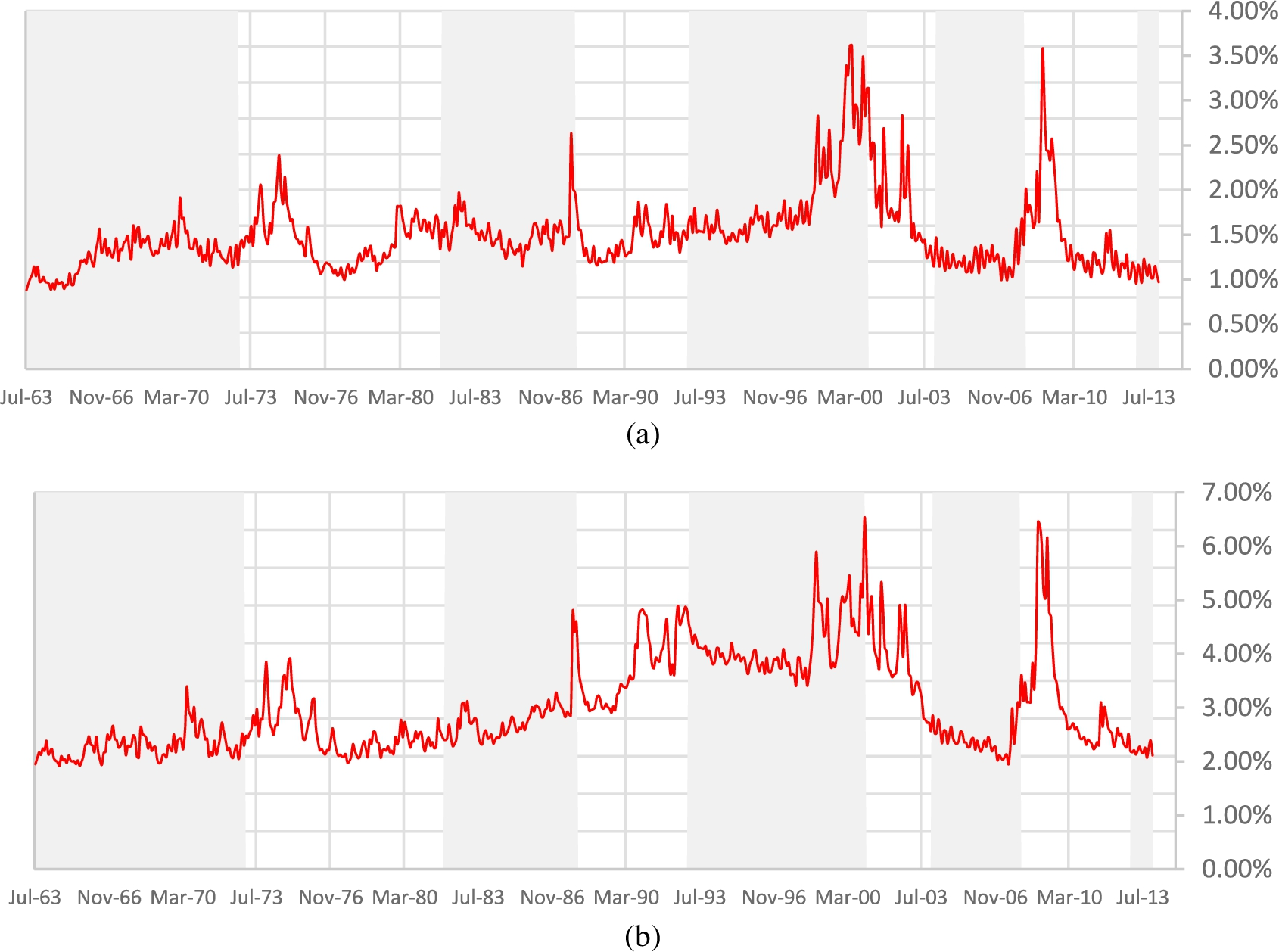
Aggregate Idiosyncratic Volatility (using the Three-Factor Model). The graphs present the aggregate idiosyncratic volatility from Jul 1963 to Dec 2013. All stocks listed on NYSE, NYSE MKT (formerly AMEX), and NASDAQ and having data on CRSP database are included in our sample. 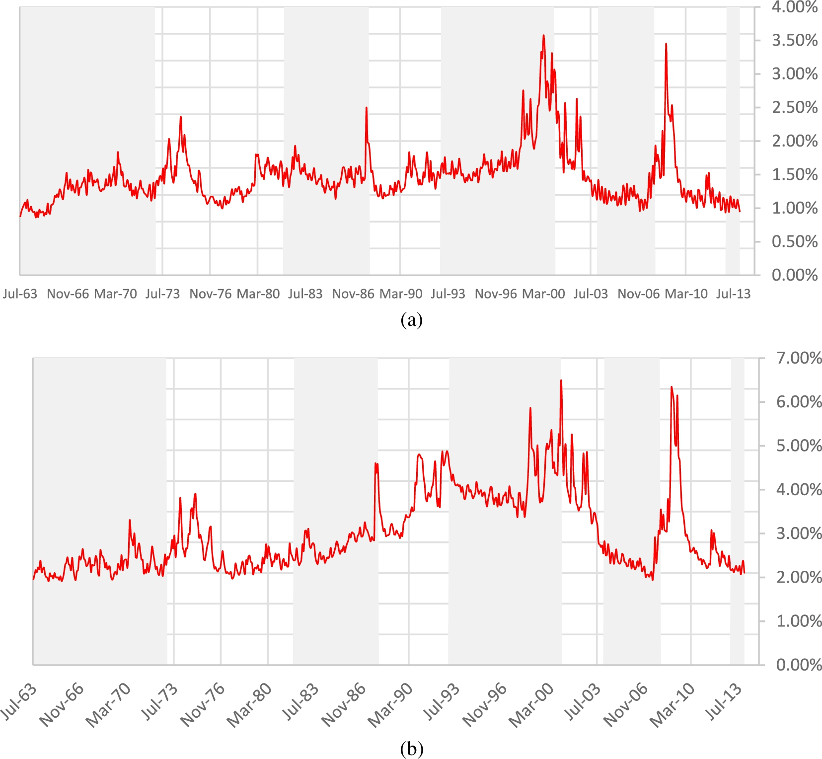Idiosyncratic volatility is calculated as the standard deviation of the residuals resulting from estimating the Fama and French [16] three factor model: $r_{i, t} - R_{f, t} = α + β_{MKT, i} (R_{m, t} - R_{f, t}) + β_{SMB, i} {SMB}_{t} + β_{HML, i} {HML}_{t} + ϵ_{t}$ . The model is estimated using daily observation every month for every stock in our sample. Next, and for every month, we estimate the value weighted and equal weighted averages for all our stocks’ idiosyncratic volatilities available within this month. We use these averages as our proxy for value-weighted and equal-weighted idiosyncratic volatility respectively. Merger Waves Periods are highlighted in grey. (a) Value Weighted Aggregate Idiosyncratic Volatility, (b) Equal Weighted Aggregate Idiosyncratic Volatility.

Fig. 2.

Aggregate Idiosyncratic Volatility (using the Five-Factor Model). The graphs present the aggregate idiosyncratic volatility from Jul 1963 to Dec 2013. All stocks listed on NYSE, NYSE MKT (formerly AMEX), and NASDAQ and having data on CRSP database are included in our sample. Idiosyncratic volatility is calculated as the standard deviation of the residuals resulting from estimating the Fama and French [17] five factor model: $r_{i, t} - R_{f, t} = α + β_{MKT, i} (R_{m, t} - R_{f, t}) + β_{SMB, i} {SMB}_{t} + β_{HML, i} {HML}_{t} + β_{RMW, i} {RMW}_{t} + β_{CMA, i} {CMA}_{t} + ϵ_{t}$ . The model is estimated using daily observation every month for every stock in our sample. Next, and for every month, we estimate the value weighted and equal weighted averages for all our stocks’ idiosyncratic volatilities available within this month. We use these averages as our proxy for value-weighted and equal-weighted idiosyncratic volatility respectively. Merger Waves Periods are highlighted in grey. (a) Value Weighted Aggregate Idiosyncratic Volatility, (b) Equal Weighted Aggregate Idiosyncratic Volatility.

Figure 3 graphs the scaled measures of idiosyncratic volatility over the sample period. Value-weighted estimates are shown based on the Fama–French [16] three-factor and Fama–French [17] five factor models. Scaled volatility measures again are computed by dividing monthly aggregate idiosyncratic volatility by monthly aggregate returns’ volatility.

Fig. 3.

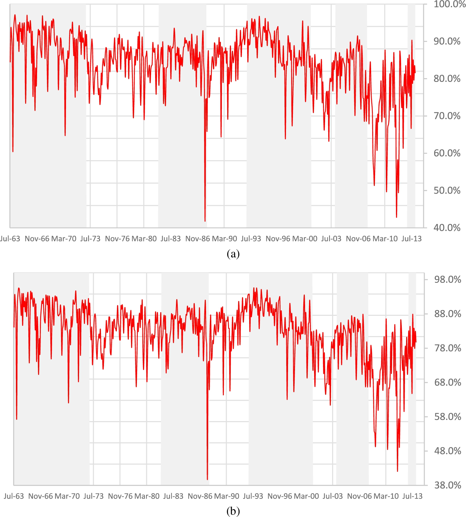
Value Weighted Scaled Idiosyncratic Volatility. The graphs present the aggregate scaled idiosyncratic volatility from Jul 1963 to Dec 2013. All stocks listed on NYSE MKT (formerly AMEX), and NASDAQ and having data on CRSP database are included in our sample. Idiosyncratic volatility is calculated as the standard deviation of the residuals resulting from estimating the Fama and French [16] three factor model: $r_{i, t} - R_{f, t} = α + β_{MKT, i} (R_{m, t} - R_{f, t}) + β_{SMB, i} {SMB}_{t} + β_{HML, i} {HML}_{t} + ϵ_{t}$ and the Fama and French [17] five factor model: $r_{i, t} - R_{f, t} = α + β_{MKT, i} (R_{m, t} - R_{f, t}) + β_{SMB, i} {SMB}_{t} + β_{HML, i} {HML}_{t} + β_{RMW, i} {RMW}_{t} + β_{CMA, i} {CMA}_{t} + ϵ_{t}$ . The model is estimated using daily observation every month for every stock in our sample. Next, and for every month, we estimate the value weighted and equal weighted averages for all our stocks’ idiosyncratic volatilities available within this month. We use these averages as our proxy for value-weighted and equal-weighted idiosyncratic volatility respectively. The Idiosyncratic volatility are scaled by the returns volatility by dividing monthly aggregate idiosyncratic volatility by monthly aggregate returns’ volatility. Merger Waves Periods are highlighted in grey. (a) Value Weighted FF3 Scaled Idiosyncratic Volatility, (b) Value Weighted FF5 Scaled Idiosyncratic Volatility.

The pattern shown in Table 3 is consistent with the paper’s basic motivation: as we move into period of high merger intensity, the importance of idiosyncratic volatility as a share of total volatility tends to rise. As we move out of a merger wave period, the role of idiosyncratic volatility falls. Similar results are observed using equal-weighted volatilities. The results presented so far are not at variance with those recently provided by Bhagwat, Dam and Harford [9]. Bhagwat, Dam and Harford [9] associate an increase in VIV with a decrease in mergers and acquisitions activities. Based on their findings, we may conclude that merger waves are usually associated with period of lower aggregate market volatility. This association does not contradict with our findings here; our aggregate idiosyncratic volatility values are lower in periods of high merger and acquisition activities. However, when scaled by aggregate volatilities, the scaled idiosyncratic volatilities are higher in periods of higher merger and acquisition activities. This highlights the importance of the firm specific risk relative to the firm total risk when periods of high merger and acquisitions intensity are considered. This is what differentiate the results presented in this section with those presented by the before mentioned authors.

Table 3

Summary of the Portfolio Performance tests for portfolios constructed using the zero investment Idiosyncratic Volatility ranked portfolios using daily data (From Appendix B, Tables A.1 to A.8). Portfolios are formed based on previous month idiosyncratic volatility using daily Returns for the idiosyncratic volatility estimation and daily returns for the subsequent performance estimation. The table reports the results related to the zero investment portfolio obtained by being long the fifth (highest idiosyncratic volatility) quintile and short the first (lowest idiosyncratic volatility) quintile

Daily Returns – Fama and French [ 16 ] Model
	Total Sample		High M&A Activity		Low M&A Activity

Alpha	-ve	Sig	-ve	Sig	-ve	Non-Sig
Average Return	-ve	Non-Sig	-ve	Sig	+ve	Non-Sig

Daily Returns – Fama and French [ 17 ] Model
	Total Sample		High M&A Activity		Low M&A Activity

Alpha	-ve	Non-Sig	-ve	Non-Sig	+ve	Sig
Average Return	-ve	Non-Sig	-ve	Sig	+ve	Non-Sig

Daily Returns – Fama and French [ 16 ] Model – Sub-Periods of High M&A Activity
	1960–1972		1982–1989		1993–2000		2004–2007		2013

Alpha	-ve	Sig	-ve	Sig	-ve	Non-Sig	-ve	Non-Sig	-ve	Non-Sig
Average Return	-ve	Non-Sig	-ve	Sig	-ve	Non-Sig	+ve	Non-Sig	+ve	Non-Sig

Daily Returns – Fama and French [ 16 ] Model – Sub-Periods of Low M&A Activity
	1973–1981		1990–1992		2001–2003		2008–2012

Alpha	-ve	Sig	+ve	Non-Sig	-ve	Non-Sig	+ve	Non-Sig
Average Return	+ve	Non-Sig	+ve	Sig	+ve	Non-Sig	+ve	Non-Sig

Daily Returns – Fama and French [ 17 ] Model – Sub-Periods of High M&A Activity
	1960–1972		1982–1989		1993–2000		2004–2007		2013

Alpha	-ve	Sig	-ve	Sig	+ve	Non-Sig	-ve	Non-Sig	+ve	Non-Sig
Average Return	-ve	Non-Sig	-ve	Sig	-ve	Non-Sig	+ve	Non-Sig	+ve	Non-Sig

Daily Returns – Fama and French [ 17 ] Model – Sub-Periods of Low M&A Activity
	1973–1981		1990–1992		2001–2003		2008–2012

Alpha	-ve	Sig	+ve	Sig	+ve	Sig	+ve	Non-Sig
Average Return	+ve	Non-Sig	+ve	Sig	-ve	Non-Sig	+ve	Non-Sig

5. The relationship between the idiosyncratic volatility puzzle and M&A activity using daily returns for performance estimation

Table 3 presents a summary of the main results for the analyses relating to the performance for alternative portfolios that are sorted into portfolios based on the previous month’s idiosyncratic volatility. The analyses use daily returns for the idiosyncratic volatility estimation and daily returns for the subsequent performance estimation. The table reports the results showing the returns from a zero investment portfolio constructed by being long the fifth (highest idiosyncratic volatility) quintile and short the first (lowest idiosyncratic volatility) quintile. Detailed results are documented in Appendix A in Tables A.1 to A.8. For presentation reasons only, we have transformed the daily performance measures into monthly performance measures.2

For both the Fama and French [16] three-factor model as well as the Fama and French [17] five factor model we corroborate the existence of the idiosyncratic volatility puzzle if the zero investment portfolio (Q5 ‘high idiosyncratic volatility portfolio’ – Q1 ‘low idiosyncratic volatility portfolio’) has a negative and significant performance measure. If in addition to the zero-investment portfolio negative significant performance, we observe a strictly decreasing trend while moving from the lowest to the highest quintile, then this would be of great support to the existence of the puzzle. However, this latter is not always observed in the literature as highlighted by Bali and Cakici [5]. We also treat a non-significant performance measure (whether positive or negative) and a positive significant performance measure as an indication that the puzzle cannot be supported by the corresponding test.

Our results show that when idiosyncratic volatility is estimated using the Fama and French [16] three factor model, the idiosyncratic volatility puzzle persists as the alpha of the zero-investment portfolio is negative and significant. However, the average return of the zero investment portfolio is not significant. This leads us to conclude that using daily return in estimating our performance measure weakens the idiosyncratic volatility puzzle but does not eliminate it (previous papers mostly use monthly returns in estimating their quintile portfolio performances instead of daily returns). On the other side, using Fama and French [17] five factor model, the puzzle is not evident: both alpha and the average return of the zero-investment portfolio are no more significant.

When the sample is divided into high M&A activity periods and the low M&A activity periods, the results that we obtain are consistent with Hypothesis 1: the idiosyncratic volatility puzzle is present in the high intensity sample and is not present in the low intensity sample. In particular, the results of our tests show that there is a negative relationship between idiosyncratic volatility and next month stock performance when performance is measured by both alpha and average returns and the three factor model is used to estimate the idiosyncratic volatility. When the five factor model is used to estimate the idiosyncratic volatility only the average returns performance measure is still negatively related to idiosyncratic volatility. For the period of low M&A activity, the relationship between idiosyncratic volatility and next month’s performance is either positive or non-significant.

Table 4
Summary of the Portfolio Performance tests for portfolios constructed using the zero investment Idiosyncratic Volatility ranked portfolios using monthly data (From Appendix B, Tables B.1 to B.8). Portfolios are formed based on previous month idiosyncratic volatility using monthly Returns for the idiosyncratic volatility estimation and monthly returns for the subsequent performance estimation. The table reports the results related to the zero investment portfolio obtained by being long the fifth (highest idiosyncratic volatility) quintile and short the first (lowest idiosyncratic volatility) quintile

Monthly Returns – Fama and French [ 16 ] Model

Total Sample High M&A Activity Low M&A Activity

Alpha -ve Sig -ve Sig -ve Sig

Average Return -ve Sig -ve Sig -ve Non-Sig

Monthly Returns – Fama and French [ 17 ] Model

Total Sample High M&A Activity Low M&A Activity

Alpha -ve Sig -ve Sig -ve Sig

Average Return -ve Sig -ve Sig -ve Non-Sig

Monthly Returns – Fama and French [ 16 ] Model – Sub-Periods of High M&A Activity

1960–1972 1982–1989 1993–2000 2004–2007 2013

Alpha -ve Sig -ve Sig -ve Sig -ve Non-Sig +ve Non-Sig

Average Return -ve Non-Sig -ve Sig -ve Non-Sig -ve Non-Sig +ve Non-Sig

Monthly Returns – Fama and French [ 16 ] Model – Sub-Periods of Low M&A Activity

1973–1981 1990–1992 2001–2003 2008–2012

Alpha -ve Sig -ve Sig +ve Non-Sig -ve Non-Sig

Average Return -ve Non-Sig -ve Sig +ve Non-Sig -ve Non-Sig

Monthly Returns – Fama and French [ 17 ] Model – Sub-Periods of High M&A Activity

1960–1972 1982–1989 1993–2000 2004–2007 2013

Alpha -ve Sig -ve Sig -ve Sig -ve Non-Sig +ve Non-Sig

Average Return -ve Non-Sig -ve Sig -ve Non-Sig +ve Non-Sig +ve Non-Sig

Monthly Returns – Fama and French [ 17 ] Model – Sub-Periods of Low M&A Activity

1973–1981 1990–1992 2001–2003 2008–2012

Alpha -ve Sig -ve Sig +ve Non-Sig -ve Non-Sig

Average Return -ve Non-Sig -ve Non-Sig -ve Non-Sig -ve Non-Sig

Given this provocative finding that is consistent with Hypothesis 1, we also estimate our performance measures over the high M&A activity sub-periods and the low M&A activity sub-periods. We find that the high M&A activity sub-periods exhibit mostly a negative significant or a non-significant relationship between performances and lagged idiosyncratic volatility whereas low M&A activity sub-periods exhibit mostly a positive significant or non-significant relationship between performances and lagged idiosyncratic volatility. These results are also obtained if we are to use the five factor model instead of the three factor model. What is intriguing is that for the high M&A activity sub-period spanning 1982 to 1989, the idiosyncratic volatility puzzle exhibit its strongest form: all performance measures of the zero investment portfolio are negative and significant. In addition, a decreasing trend can be clearly observed.3

In a nutshell, our results seem to support that the idiosyncratic volatility puzzle intensifies in high M&A activity periods and weakens in low M&A activity periods, consistent with Hypothesis 1.

6. The relationship between the idiosyncratic volatility puzzle and M&A activity using monthly returns for performance estimation

Much of the previous literature on the idiosyncratic volatility puzzle uses monthly returns to estimate the performances of the quintile portfolios obtained after sorting stocks based on their idiosyncratic volatility, we repeat our tests using our monthly portfolio returns.

Table 4 presents a summary of the main results for the analyses relating to the performance for alternative portfolios that are sorted into portfolios based on the previous month’s idiosyncratic volatility. The analyses use daily returns for the idiosyncratic volatility estimation and monthly returns for the subsequent performance estimation. The table reports the results showing the returns from a zero investment portfolio constructed by being long the fifth (highest idiosyncratic volatility) quintile and short the first (lowest idiosyncratic volatility) quintile. Detailed results are documented in Appendix B in Tables B.1 to B.8.

In contrast to the results using daily returns, we find that the idiosyncratic volatility puzzle is now strong for our total sample: both the alpha and the average returns of the zero-investment portfolio are negative and significant. Second, using the Fama and French [17] five factor model does not mitigate the puzzle as reported for the daily performance measure: both alpha and average returns of the zero-investment portfolio are still negative and significant. Third when we divide the sample into high M&A activity periods versus low M&A activity period it seems that the puzzle is still strong for the high M&A activity period: both alpha and average return are negative and significant for the zero-investment portfolio. For the period of low M&A activity period: both alpha and average return of the zero investment portfolio are negative but only the alpha is significant. The idiosyncratic volatility puzzle exists mildly for the low M&A activity period but its effect is still weaker than in the high M&A activity period. Consistent with the results using daily data, the strongest idiosyncratic volatility effect is observed still in the period spanning from 1982 to 1989.

To summarize, our results using monthly returns are supportive of Hypothesis 1 supporting a link between the IV puzzle and M&A intensity.

7. The relationship between the exposure to the common idiosyncratic volatility factor and M&A activity

Herskovic et al. [23] shows that shocks to the common idiosyncratic volatility (CIV) factor are priced and that stocks with lower CIV-exposure in a particular month perform better than their higher CIV-exposure peers in the next month. CIV factor is correlated with income risk faced by households, not related to risk of firms in M&A. In this section, we test whether this relationship is persistent across periods of high and low mergers and acquisitions activities.

7.1. Sorting stocks into portfolios based on lagged exposure to the common idiosyncratic volatility factor as per Herskovic et al. [23]

We construct our Common Idiosyncratic volatility factor following the approach of Herskovic et al. [23]. For each month, we estimate a regression of daily individual stock returns on the CRSP value-weighted index (our proxy for market return in this case: $R_{m, t}$ ) for all the CRSP stocks with non-missing data for that month as per the model below: $\begin{matrix} r_{i, t} = α_{i} + β_{MKT, i} (R_{m, t}) + ϵ_{t} \end{matrix}$ Next individual stocks monthly variances are estimated as the variance of the residuals resulting from the above model: ${Idiosyncratic_Variance}_{i, t} = σ^{2} (ϵ_{t})$ . Once individual variances are obtained, an equal-weighted average of them is calculated for each month in our sample. This latter would serve as our Common Idiosyncratic Volatility (CIV) factor. Shocks to the CIV factors are obtained as the month to month difference between the previously constructed CIV values.

Herskovic et al. [23] also compute a Market Variance (MV) factor as control variable for testing the predictive power of the CIV factor. Following their approach, we also construct our MV factor by estimating the variance of the CRSP value-weighted index each month by relying on the daily observations within this month. Similar to CIV shocks, MV shocks are obtained as the first difference in the MV factor from one month to the other.

Once CIV and MV shocks are obtained, and for every month and for every stock in our sample, monthly stocks excess returns are regressed on CIV and MV shocks using a 60-month historical window. As in the idiosyncratic volatility analysis, we limited the sample to stocks with share codes 10, 11 and 12. We require stocks to have at least 60 historical monthly return observations to be kept in our sample of stocks for a given that month. These regressions would lead to a monthly series of stocks’ exposure to CIV shocks and MV shocks; the CIV-Betas and the MV-Betas.

Next, we sort stocks into equal-weighted quintile portfolios based on their CIV-Betas and estimate the next month returns for these portfolios as well as the next month return on a self-financing portfolio that is long the highest CIV-Beta quintile portfolio and short the lowest CIV-Beta quintile portfolio. We use equally weighted portfolios as per Herskovic et al. [23]. In addition, both the Fama and French [16] three factor and Fama and French [17] five factor models are used to estimate the stocks’ idiosyncratic variances and in turn, the common idiosyncratic volatility factor. Monthly first differences are used to generate the factors’ shocks. The exposure to the CIV factor is obtained by regressing monthly stocks excess-returns on the CIV-factor, the Market Variance factor, the SMB Variance factor as well as the HML Variance factor for the case of Fama and French [16] three factor model benchmark.

Table 5
Summary of the Portfolio Performance tests for portfolios constructed using the zero investment factor Idiosyncratic Volatility ranked portfolios using monthly data (From Appendix C, Tables C.1 to C.8). Portfolios are formed based on previous month exposure to factor idiosyncratic volatility using monthly, suing the Herskovic et al. [23] methodology. Returns for the idiosyncratic volatility estimation and monthly returns for the subsequent performance estimation. The table reports the results related to the zero investment portfolio obtained by being long the fifth (highest idiosyncratic volatility) quintile and short the first (lowest idiosyncratic volatility) quintile The Table reports the results related to the zero investment portfolio obtained by being long the fifth (highest exposure to common idiosyncratic volatility factor) quintile and short the first (lowest exposure to common idiosyncratic volatility factor) quintile

CIV Constructed based on Market Model vs. CIV Constructed based on Fama and French [ 16 ] Three Factor Model vs. CIV Constructed based on Fama and French [ 17 ] Five Factor Model

Market Model CIV Three Factor Model CIV Five Factor Model CIV

Three Factor Alpha -ve Sig -ve Sig -ve Sig

Five Factor Alpha -ve Sig -ve Sig -ve Sig

Average Return -ve Sig -ve Sig -ve Sig

CIV Constructed based on Market Model

Total Sample High M&A Activity Low M&A Activity

Three Factor Alpha -ve Sig -ve Sig -ve Sig

Five Factor Alpha -ve Sig -ve Sig -ve Sig

Average Return -ve Sig -ve Sig -ve Sig

CIV Constructed based on Market Model – Sub-Periods of High M&A Activity

1960–1972 1982–1989 1993–2000 2004–2007 2013

Three Factor Alpha -ve Sig -ve Sig -ve Sig -ve Sig -ve Non-Sig

Five Factor Alpha -ve Sig -ve Sig -ve Sig -ve Non-Sig -ve Non-Sig

Average Return -ve Non-Sig +ve Non-Sig -ve Sig -ve Non-Sig -ve Non-Sig

CIV Constructed based on Market Model – Sub-Periods of Low M&A Activity

1973–1981 1990–1992 2001–2003 2008–2012

Three Factor Alpha -ve Sig -ve Sig -ve Non-Sig -ve Non-Sig

Five Factor Alpha -ve Sig -ve Sig -ve Non-Sig -ve Sig

Average Return -ve Sig -ve Non-Sig -ve Non-Sig -ve Non-Sig

Table 6

Summary of the Results Presented in Table 32 to 37. Summary of the main results related to sorting portfolios based on previous month exposure to common factor idiosyncratic volatility following Herskovic et al. [23] Methodology but using 12 months to estimate the exposure to CIV instead of 60 months. The Table reports the results related to the zero investment portfolio obtained by being long the fifth (highest exposure to common idiosyncratic volatility factor) quintile and short the first (lowest exposure to common idiosyncratic volatility factor) quintile

CIV Constructed based on Market Model
	High M&A Activity		Low M&A Activity

Three Factor Alpha	-ve	Sig	-ve	Sig
Five Factor Alpha	-ve	Sig	-ve	Sig
Average Return	-ve	Non-Sig	-ve	Sig

CIV Constructed based on Market Model – Sub-Periods of High M&A Activity
	1960–1972		1982–1989		1993–2000		2004–2007		2013

Three Factor Alpha	-ve	Sig	-ve	Sig	-ve	Non-Sig	+ve	Non-Sig	+ve	Sig
Five Factor Alpha	-ve	Sig	-ve	Sig	-ve	Non-Sig	+ve	Non-Sig	+ve	Sig
Average Return	-ve	Non-Sig	-ve	Non-Sig	-ve	Non-Sig	+ve	Non-Sig	-ve	Non-Sig

CIV Constructed based on Market Model – Sub-Periods of Low M&A Activity
	1973–1981		1990–1992		2001–2003		2008–2012

Three Factor Alpha	-ve	Sig	-ve	Sig	-ve	Non-Sig	-ve	Sig
Five Factor Alpha	-ve	Sig	-ve	Sig	+ve	Non-Sig	-ve	Sig
Average Return	-ve	Non-Sig	-ve	Non-Sig	-ve	Non-Sig	-ve	Non-Sig

Table 5 presents a summary of the main results of the Portfolio Performance tests for portfolios constructed using the zero investment factor using a fifty-month estimation window. The table reports the results showing the returns from a zero investment portfolio constructed by being long the fifth (highest idiosyncratic volatility) quintile and short the first (lowest idiosyncratic volatility) quintile. Detailed results are documented in Appendix C in Tables C.1 to C.8.

At first, we check whether the results documented by Herskovic et al. [23] are model specific. The authors build their work by estimating the idiosyncratic volatility relying the single factor market model. Consistent with the factor model reported in this paper, we redo their tests using the Fama and French [16] and the Fama and French [17] factor models. Our findings are consistent with those reported by Herskovic et al. [23] and similar across the different model specifications; the negative relationship between stock performance and lagged exposure to the CIV factor is significant whether we use the Market Model, the Fama and French [16] three factor model or the Fama and French [17] five factor model. The results are also robust to whether we use average return, Fama and French [16] three factor alpha or Fama and French [17] five factor alpha to estimate our portfolio performances.

Since the different factor models exhibit similar behavior, we rely on the market model used by Herskovic et al. [23] to test whether the relationship between expected return and lagged exposure to the CIV factor is affected by mergers and acquisitions activities. Our findings are not supportive of Hypothesis 2. M&A activity does not affect the relationship between expected returns and lagged exposure to the CIV factor: the relationship is negative and significant for the high M&A activity period, the low M&A activity period as well as most of their constituents’ sub-periods. Hence the results do not support Hypothesis 2.

Table 7

Summary of the Results Presented in Table 38 to 43. Summary of the main results related to sorting portfolios based on previous month exposure to common factor idiosyncratic volatility following Herskovic et al. [23] Methodology but using 12 months to estimate the exposure to CIV instead of 60 months and removing the first year of every sub-sample period. The Table reports the results related to the zero investment portfolio obtained by being long the fifth (highest exposure to common idiosyncratic volatility factor) quintile and short the first (lowest exposure to common idiosyncratic volatility factor) quintile

CIV Constructed based on Market Model
	High M&A Activity		Low M&A Activity

Three Factor Alpha	-ve	Sig	-ve	Sig
Five Factor Alpha	-ve	Sig	-ve	Sig
Average Return	-ve	Non-Sig	-ve	Sig

CIV Constructed based on Market Model – Sub-Periods of High M&A Activity
	1961–1972		1983–1989		1994–2000		2005–2007

Three Factor Alpha	-ve	Sig	-ve	Sig	-ve	Non-Sig	+ve	Non-Sig
Five Factor Alpha	-ve	Sig	-ve	Sig	-ve	Non-Sig	+ve	Non-Sig
Average Return	-ve	Non-Sig	-ve	Non-Sig	-ve	Non-Sig	+ve	Sig

CIV Constructed based on Market Model – Sub-Periods of Low M&A Activity
	1974–1981		1991–1992		2002–2003		2009–2012

Three Factor Alpha	-ve	Sig	-ve	Non-Sig	+ve	Non-Sig	-ve	Non-Sig
Five Factor Alpha	-ve	Sig	-ve	Non-Sig	+ve	Sig	-ve	Non-Sig
Average Return	-ve	Non-Sig	-ve	Non-Sig	+ve	Non-Sig	-ve	Sig

These reported findings might be confounded due to the long window (60 months) used to estimate the exposure to the CIV factor. A 60 month window might easily span more than one adjacent sub-period and cover both high and low M&A activity periods. Hence, we redo our tests while re-estimating stocks’ exposure to the CIV factor over a 12 months estimation window rather than a 60 months window. The results of these tests are summarized in Table 6 with detailed estimates shown in Appendix D, Tables D.1 to D.6.

Again, we fail to detect observable differences between the high and low M&A activity periods and their corresponding sub-periods. Considering that the first year of every sub-period would still rely on some observations from the previous sub-period, we decided to remove the first year of every sub-period while estimating our portfolio performances. Table 7 summarizes the results that are reported in Appendix E, Tables E.1 to E.6.

As we notice these extra tests did not change our initial findings: stock exposure to the CIV factor is still negatively related to stocks expected performances independent of the M&A activity.

When conditioned on M&A activity, the difference in behavior exhibited by stocks while ranked based on their previous month idiosyncratic volatility and their previous month exposure to the common idiosyncratic volatility factor reveals that these two measures are capturing different firms’ characteristics or risk exposure.

8. Conclusion

The idiosyncratic volatility puzzle revolves around a negative relationship between stocks’ idiosyncratic volatility and next month’s expected performance. This observation is documented by Ang et al. [2] and has been a topic of considerable interest in the literature. In this paper, we establish a relationship between the intensity of merger and acquisition activity and the idiosyncratic volatility puzzle. In particular, we demonstrate that the puzzle is stronger in periods of high merger and acquisition activity than in periods of low merger and acquisition activity. This suggests the existence of a relationship between the intensity of M&A activity and the way in which idiosyncratic volatility affects stock expected returns. We classify nationwide merger waves as periods of high M&A activity and the periods when no waves are reported as low M&A activity. The M&A literature suggest that a nationwide M&A wave is a clustering of a series of M&A waves in different industries. This clustering is mainly boosted or facilitated by liquidity and misvaluations. The industry waves themselves are usually initiated by internal shocks that are usually the results of technological changes in the corresponding industry. Merger waves are also associated with changes in legal and regulatory regimes. Both industry internal shocks and market misvaluation create uncertainty related to the future prospects of firms that are varying from industry to another and from one company to another within the same industry according to the exposure of this company to the new way of the industry operation. In addition, a company involved in an M&A deal would pass through a period of instability related to its own future prospects as the deal being negotiated and until both firms combine their operation under one management, one vision and one culture. Uncertainty about the firm’s future prospects induces shocks to firm’s idiosyncratic volatility that enhance the negative relationship between idiosyncratic volatility and next month expected returns.

We show that the link between idiosyncratic volatility puzzle and mergers and acquisitions is robust to whether or not we use daily or monthly data in the analyses, as well as to different model specifications: whether we use the Fama and French [16] three factor model or the Fama and French [17] five factor model to estimate our idiosyncratic volatility.

Our attempts to link the mergers and acquisitions activity to the negative relationship between stocks’ expected returns and previous month exposure to the common idiosyncratic volatility (CIV) factor proved futile. This leads us to conclude that firms’ idiosyncratic volatility and firms’ exposure to the CIV factor are catching two distinct firms’ characteristics or firms’ risk exposure. M&A activity can in part explain the idiosyncratic volatility puzzle, but it does not subsume the negative relationship between CIV exposure and firm returns. Our paper identifies a number of questions and challenges for future research. One important challenge is to isolate links between factors responsible for different merger waves that may account for the variations in the intensity of the IV puzzle. Our results show that the idiosyncratic volatility puzzle is stronger in high M&A activity periods. Indeed, during the 1982–89 merger wave period all performance measures of the zero investment portfolio are negative and significant, As noted by Betton, Eckbo and Thorburn [6], this period has been dubbed as the refocusing wave, where several mergers were either designed for firms to specialize their operations or to downsize. This is also a period in which the number of hostile bids reached a peak. To the extent that misvaluations that lead to the IV puzzle are greater for firms that restructure, or downsize or that the takeovers are hostile as opposed to friendly bids remains as issues for future investigation.

Footnotes

Acknowledgements

We would like to thank the Editor, Charles Tapiero, the anonymous referees, and seminar participants at the 2017 Midwest Finance Association Meetings, the 2017 Global Finance Meetings, AFFI Meetings, IRMC Meetings, and MFS meetings for their helpful comments and suggestions. Financial support to Switzer (the Van Berkom Chair of Small-Cap Equities) from the SSHRC and the Autorité des Marchés Financiers is gratefully acknowledged.

See Cretin, Dieudonné and Bouacha [].

We use the following formula to transfer daily effective returns into monthly effective returns: $r_{effective monthly} = {(1 + r_{effective daily})}^{30} - 1$ .

In unreported tests, we limit this sub-period to span from 1982 to 1987 but similar results are obtained.

References

Ahern

K.R.

and Harford

, The importance of industry links in merger waves, Journal of Finance 69(2) (2014), 527–576. doi:10.1111/jofi.12122.

Ang

Hodrick

R.J.

Xing

and Zhang

, The cross-section of volatility and expected returns, Journal of Finance 61(1) (2006), 259–299. doi:10.1111/j.1540-6261.2006.00836.x.

Ang

Hodrick

R.J.

Xing

and Zhang

, High idiosyncratic volatility and low returns: International and further US evidence, Journal of Financial Economics 91(1) (2009), 1–23. doi:10.1016/j.jfineco.2007.12.005.

Ang

J.S.

and Cheng

, Direct evidence on the market-driven acquisition theory, Journal of Financial Research 29(2) (2006), 199–216. doi:10.1111/j.1475-6803.2006.00174.x.

Bali

T.G.

and Cakici

, Idiosyncratic volatility and the cross section of expected returns, Journal of Financial and Quantitative Analysis 43(1) (2008), 29–58. doi:10.1017/S002210900000274X.

Betton

Eckbo

B.E.

and Thorburn

K.S.

, Corporate takeovers, in: Handbook of Corporate Finance: Empirical Corporate Finance Eckbo

B.E.

, ed., Elsevier/North-Holland Handbook of Finance Series, Vol. 2, 2008, pp. 291–430, Ch. 15. doi:10.1016/B978-0-444-53265-7.50007-X.

Bhagwat

Dam

R.A.

and Harford

, The real effects of uncertainty on merger activity, Review of Financial Studies (2014), forthcoming, May 2016.

Blume

M.E.

and Stambaugh

R.F.

, Biases in computed returns: An application to the size effect, Journal of Financial Economics 12(3) (1983), 387–404. doi:10.1016/0304-405X(83)90056-9.

Boehme

R.D.

Danielsen

B.R.

Kumar

and Sorescu

S.M.

, Idiosyncratic risk and the cross-section of stock returns: Merton (1987) meets Miller (1977), Journal of Financial Markets 12(3) (2009), 438–468. doi:10.1016/j.finmar.2009.01.004.

10.

Brockman

and Schutte

, Is idiosyncratic volatility priced? The international evidence, Unpublished working paper, University of Missouri U Columbia, 2007.

11.

Chen

and Petkova

, Does idiosyncratic volatility proxy for risk exposure?, Review of Financial Studies 25(9) (2012), 2745–2787. doi:10.1093/rfs/hhs084.

12.

Cretin

Dieudonné

and Bouacha

, M&A activity: Where are we in the cycle?, 2014. Electronic copy available at: http://ssrn.com/abstract=2504412.

13.

Dong

Hirshleifer

Richardson

and Teoh

S.H.

, Does investor misvaluation drive the takeover market?, Journal of Finance 61(2) (2006), 725–762. doi:10.1111/j.1540-6261.2006.00853.x.

14.

Duarte

Kamara

Siegel

and Sun

, The systematic risk of idiosyncratic volatility, 2014, Available at SSRN 1905731.

15.

Duchin

and Schmidt

, Riding the merger wave: Uncertainty, reduced monitoring, and bad acquisitions, Journal of Financial Economics 107 (2013), 69–88. doi:10.1016/j.jfineco.2012.07.003.

16.

Fama

E.F.

and French

K.R.

, Common risk factors in the returns on stocks and bonds, Journal of Financial Economics 33 (1993), 3–56. doi:10.1016/0304-405X(93)90023-5.

17.

Fama

E.F.

and French

K.R.

, A five-factor asset pricing model, Journal of Financial Economics 116(1) (2015), 1–22. doi:10.1016/j.jfineco.2014.10.010.

18.

, Idiosyncratic risk and the cross-section of expected stock returns, Journal of Financial Economics 91(1) (2009), 24–37. doi:10.1016/j.jfineco.2008.02.003.

19.

Goyal

and Santa-Clara

, Idiosyncratic risk matters!, Journal of Finance 58(3) (2003), 975–1007. doi:10.1111/1540-6261.00555.

20.

Guo

and Savickas

, Average idiosyncratic volatility in G7 countries, Review of Financial Studies 21(3) (2008), 1259–1296. doi:10.1093/rfs/hhn043.

21.

Han

and Lesmond

, Liquidity biases and the pricing of cross-sectional idiosyncratic volatility, Review of Financial Studies 24(5) (2011), 1590–1629. doi:10.1093/rfs/hhq140.

22.

Harford

, What drives merger waves?, Journal of financial economics 77(3) (2005), 529–560. doi:10.1016/j.jfineco.2004.05.004.

23.

Herskovic

Kelly

Lustig

and Van Nieuwerburgh

, The common factor in idiosyncratic volatility: Quantitative asset pricing implications, Journal of Financial Economics 119(2) (2016), 249–283.

24.

Hou

and Loh

, Have we solved the idiosyncratic volatility puzzle?, Journal of Financial Economics 121(1) (2016), 167–194. doi:10.1016/j.jfineco.2016.02.013.

25.

Huang

Liu

Rhee

S.G.

and Zhang

, Return reversals, idiosyncratic risk, and expected returns, Review of Financial Studies (2009), hhp015.

26.

Jiang

G.J.

and Yao

, The information content of idiosyncratic volatility, Journal of Financial and Quantitative Analysis 44(1) (2009), 1–28. doi:10.1017/S0022109009090073.

27.

Jones

and Rhodes-Kropf

, The price of diversifiable risk in venture capital and private equity, Working paper, Columbia University, 2003.

28.

Jovanovic

and Rousseau

P.L.

, Mergers and technological change: 1885–1998, Unpublished working paper, 2001.

29.

Jovanovic

and Rousseau

P.L.

, The Q-theory of mergers (No. w8740), National Bureau of Economic Research, 2002.

30.

Lang

Stulz

and Walkling

, Managerial performance, Tobin’s q, and the gains from successful tender offers, Journal of Financial Economics 24 (1989), 137–154. doi:10.1016/0304-405X(89)90075-5.

31.

Levy

, Equilibrium in an imperfect market: A constraint on the number of securities in the portfolio, American Economic Review 68 (1978), 643–658.

32.

Maksimovic

and Phillips

, The market for corporate assets: Who engages in mergers and asset sales and are there efficiency gains?, Journal of Finance 56(6) (2001), 2019–2065. doi:10.1111/0022-1082.00398.

33.

Malkiel

and Xu

, Idiosyncratic risk and security returns, Working Paper, University of Texas at Dallas, Richardson, 2006.

34.

Martynova

and Renneboog

, A century of corporate takeovers: What have we learned and where do we stand?, Journal of Banking & Finance 32(10) (2008), 2148–2177. doi:10.1016/j.jbankfin.2007.12.038.

35.

Merton

R.C.

, A simple model of capital market equilibrium with incomplete information, Journal of Finance 42(3) (1987), 483–510. doi:10.1111/j.1540-6261.1987.tb04565.x.

36.

Mitchell

M.L.

and Mulherin

J.H.

, The impact of industry shocks on takeover and restructuring activity, Journal of Financial Economics 41(2) (1996), 193–229. doi:10.1016/0304-405X(95)00860-H.

37.

Rhodes-Kropf

Robinson

D.T.

and Viswanathan

, Valuation waves and merger activity: The empirical evidence, Journal of Financial Economics 77(3) (2005), 561–603. doi:10.1016/j.jfineco.2004.06.015.

38.

Rhodes-Kropf

and Viswanathan

, Market valuation and merger waves, Journal of Finance 59(6) (2004), 2685–2718. doi:10.1111/j.1540-6261.2004.00713.x.

39.

Servaes

, Tobin’s Q and the gains from takeovers, The Journal of Finance 46(1) (1991), 409–419. doi:10.1111/j.1540-6261.1991.tb03758.x.

40.

Shleifer

and Vishny

R.W.

, Stock market driven acquisitions, Journal of Financial Economics 70(3) (2003), 295–311. doi:10.1016/S0304-405X(03)00211-3.

41.

Spiegel

and Wang

, Cross-sectional variation in stock returns: Liquidity and idiosyncratic risk, Unpublished working paper, 2007.

42.

Switzer

L.N.

and Picard

, Idiosyncratic volatility, momentum, liquidity, and expected stock returns in developed and emerging markets, Multinational Finance Journal 19(3) (2015), 169–221. doi:10.17578/19-3-2.

Monthly Returns – Fama and French [ 16 ] Model
	Total Sample		High M&A Activity		Low M&A Activity

Alpha	-ve	Sig	-ve	Sig	-ve	Sig
Average Return	-ve	Sig	-ve	Sig	-ve	Non-Sig

Monthly Returns – Fama and French [ 17 ] Model
	Total Sample		High M&A Activity		Low M&A Activity

Alpha	-ve	Sig	-ve	Sig	-ve	Sig
Average Return	-ve	Sig	-ve	Sig	-ve	Non-Sig

CIV Constructed based on Market Model vs. CIV Constructed based on Fama and French [ 16 ] Three Factor Model vs. CIV Constructed based on Fama and French [ 17 ] Five Factor Model
	Market Model CIV		Three Factor Model CIV		Five Factor Model CIV

Three Factor Alpha	-ve	Sig	-ve	Sig	-ve	Sig
Five Factor Alpha	-ve	Sig	-ve	Sig	-ve	Sig
Average Return	-ve	Sig	-ve	Sig	-ve	Sig